Robust Cylindrical Panorama Stitching for Low-Texture Scenes Based on Image Alignment Using Deep Learning and Iterative Optimization

Abstract
:1. Introduction
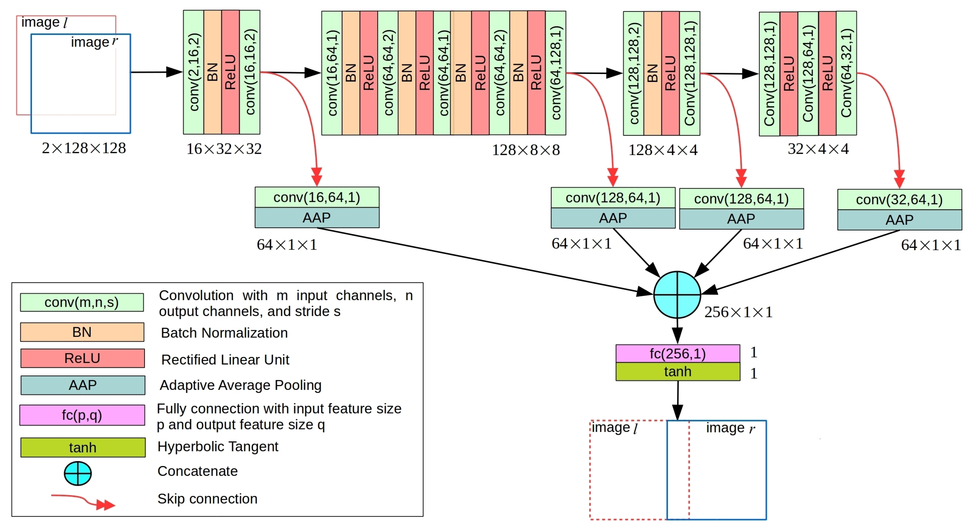
- A novel light-weight regression convolutional neural network (CNN) architecture called ShiftNet, able to handle low-texture environments properly, is proposed to predict robust shift estimates. ShiftNet can be trained in an end-to-end fashion using a large synthetic dataset generated from a publicly available image dataset. The performance of ShiftNet is superior to recent CNN models in terms of both model size and inference accuracy.
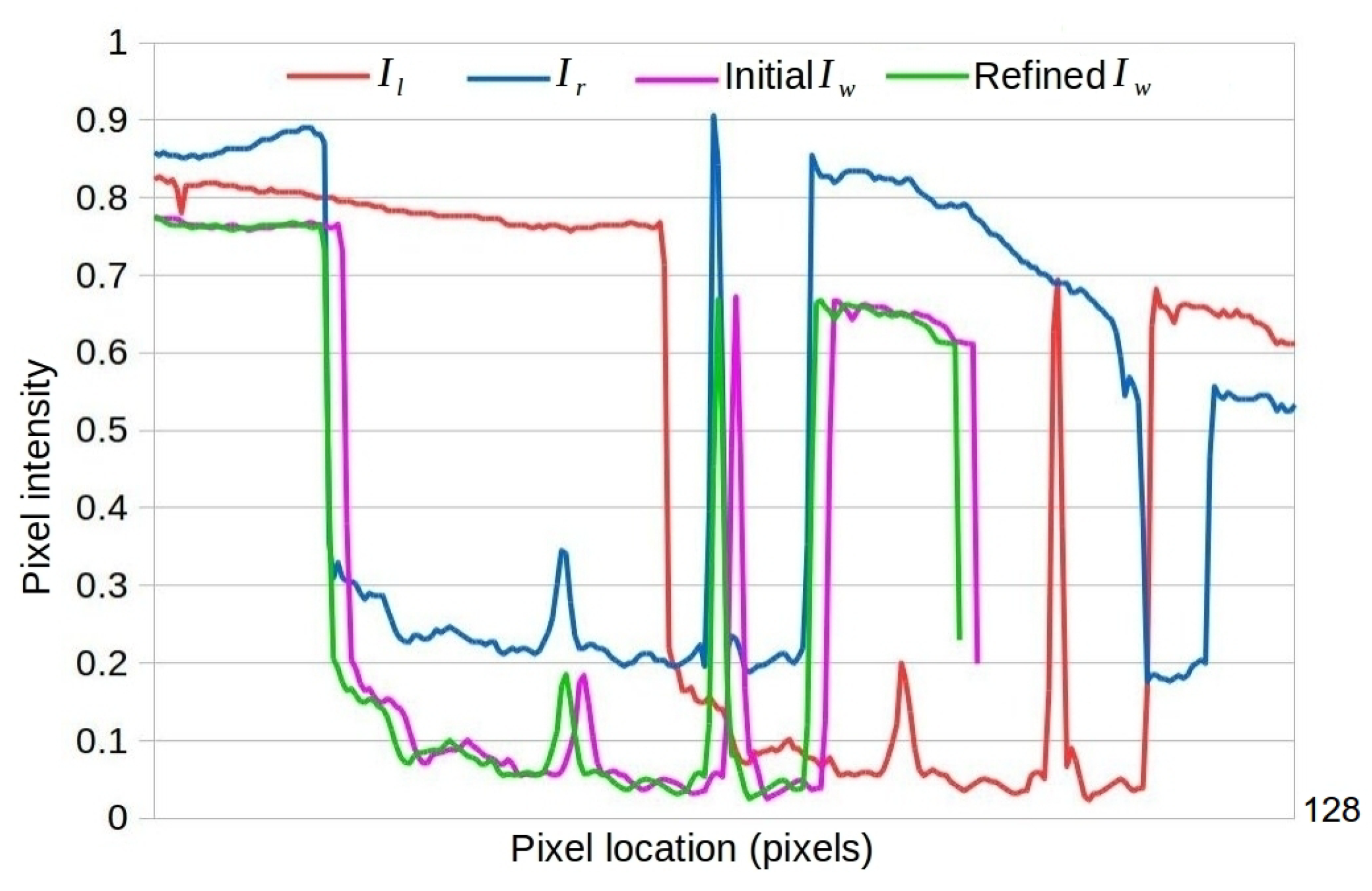
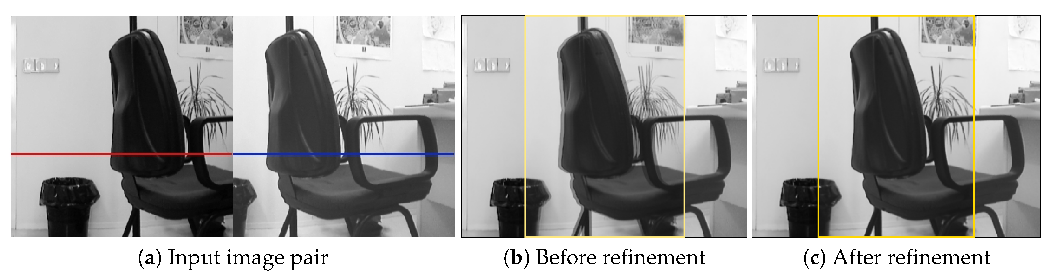
- A global illumination invariant sub-pixel refinement algorithm is proposed to improve the accuracy of the initial estimate obtained by ShiftNet under either a strict horizontal translation motion or a translate and scale motion assumption. The refinement procedure is essential for cylindrical panorama stitching because the outputs of a CNN model are not accurate enough to produce visually pleasing results.
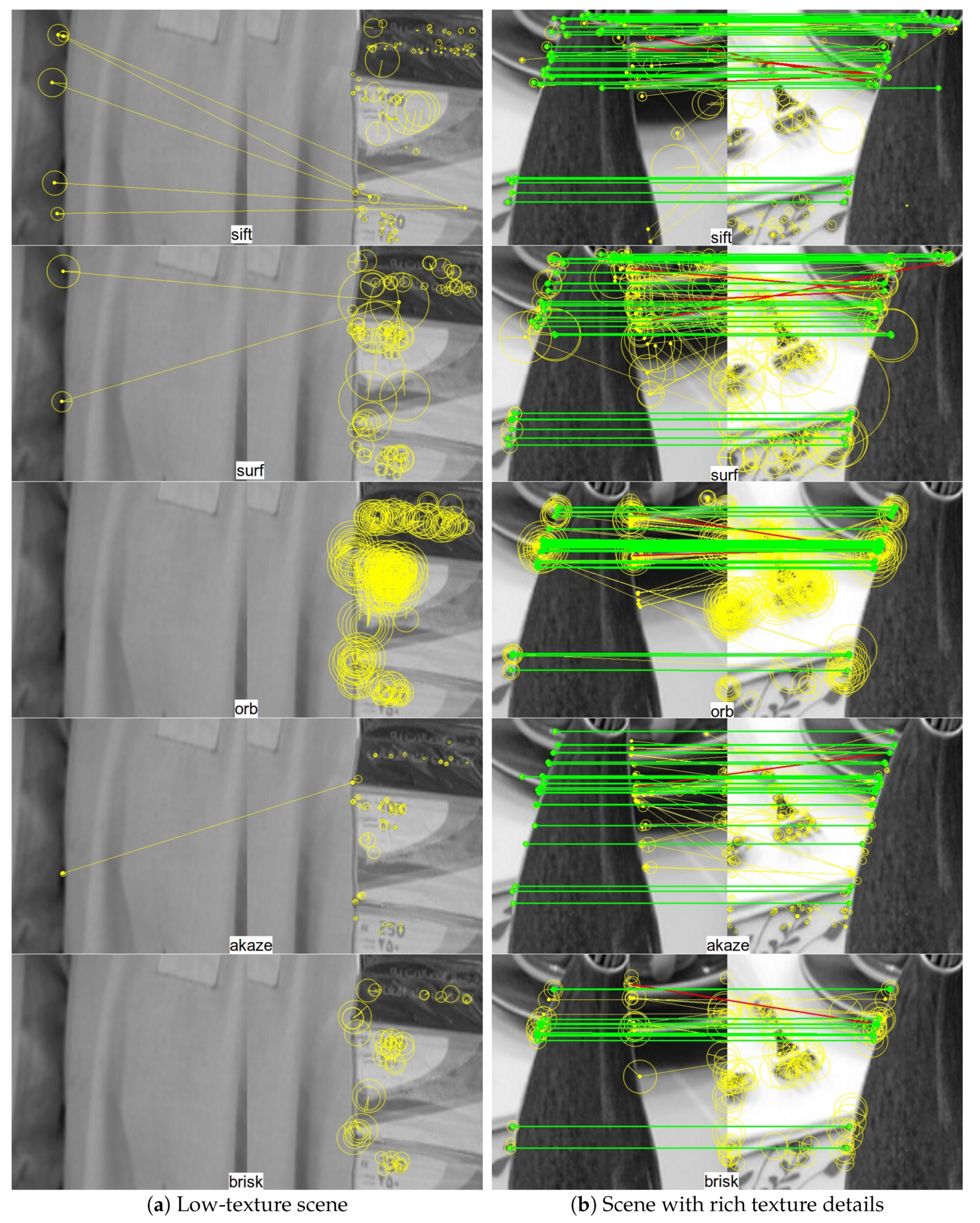
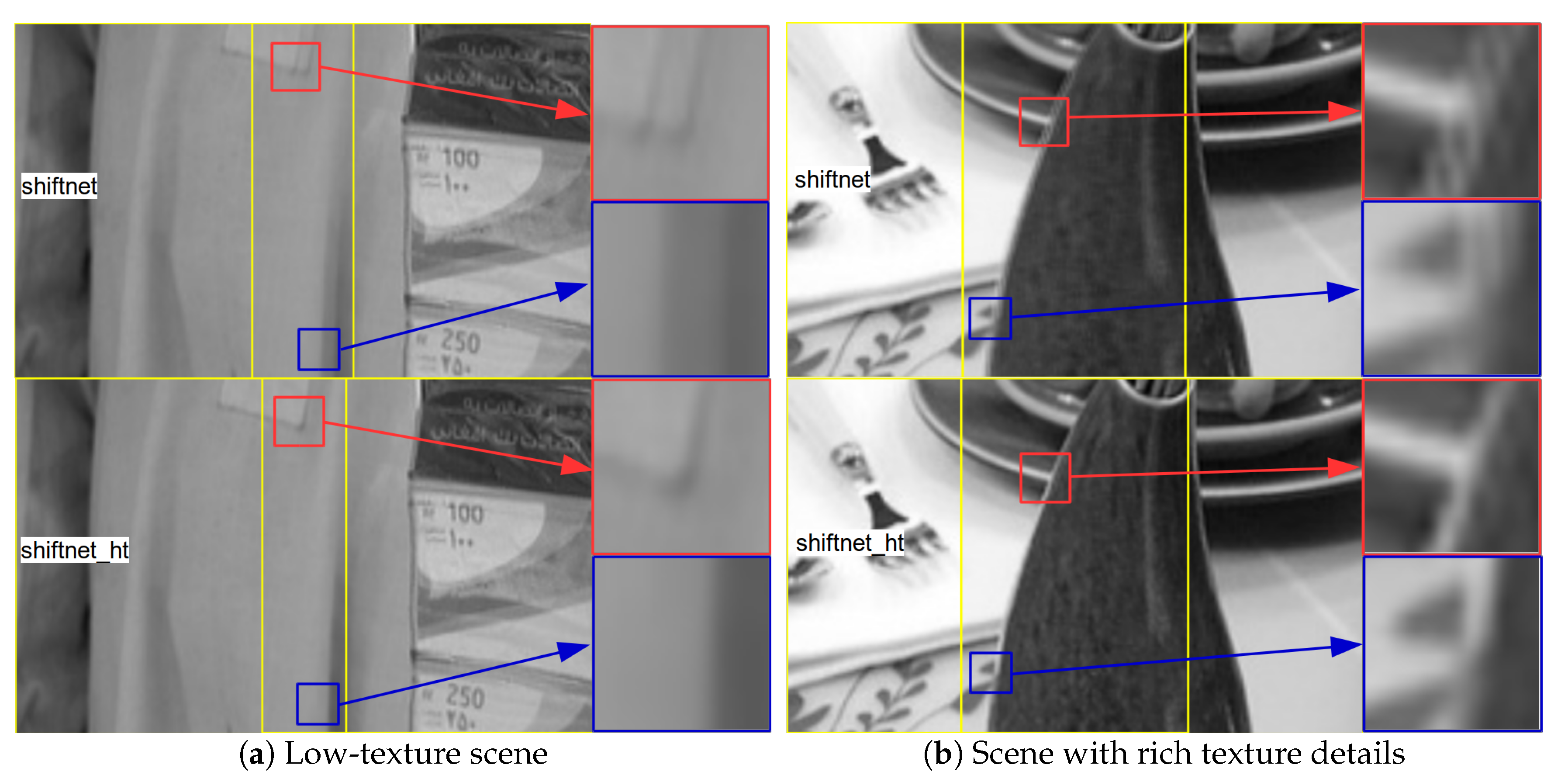
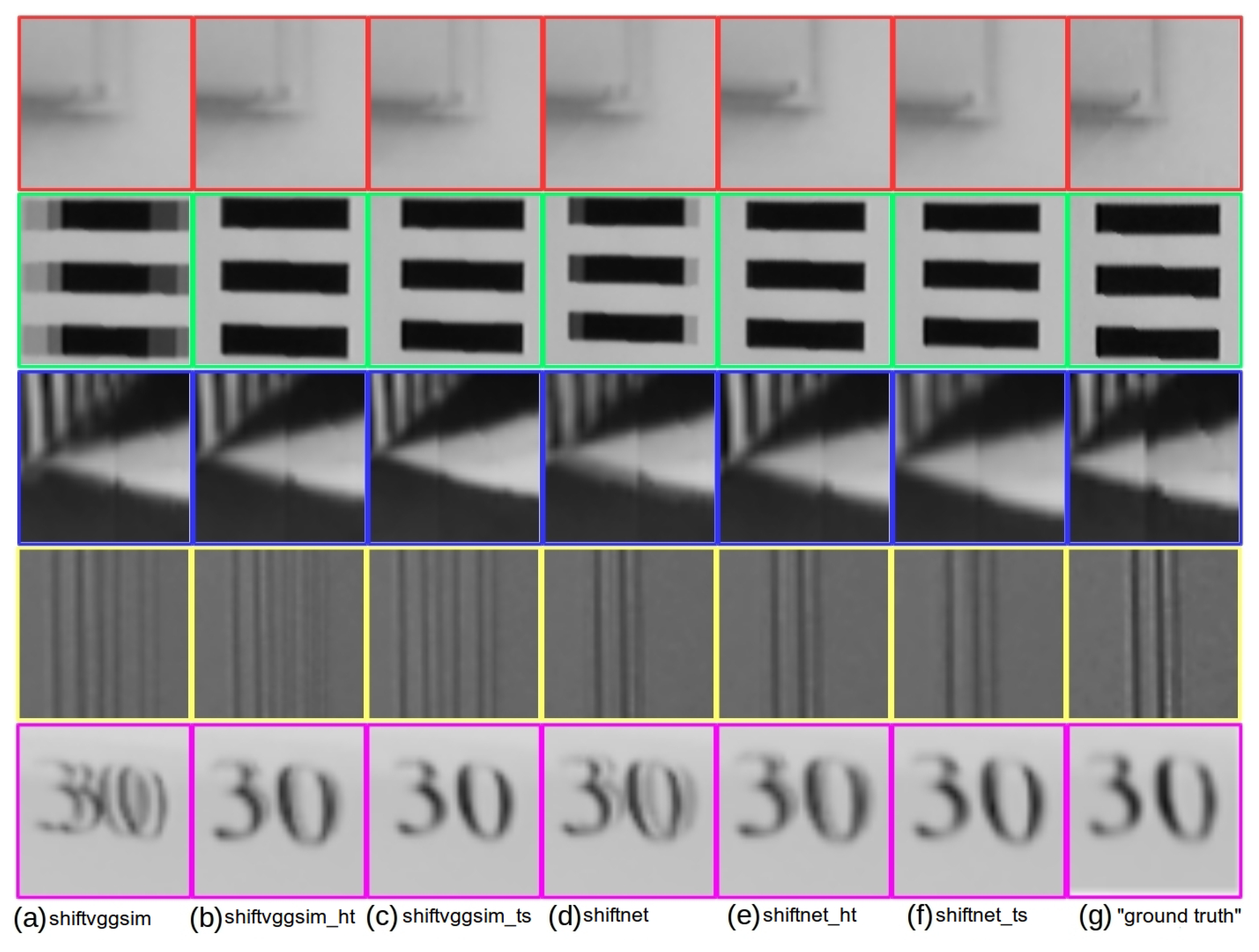
- Extensive experiments on a synthetic dataset rendered photo-realistic images, and real images were then tested to throughly evaluate the performance of the proposed method and comparative methods. Both qualitative and quantitative experimental results for challenging low-texture environments demonstrated significant improvements over traditional feature based methods and recent deep learning based methods.
2. Related Works
3. Proposed Method
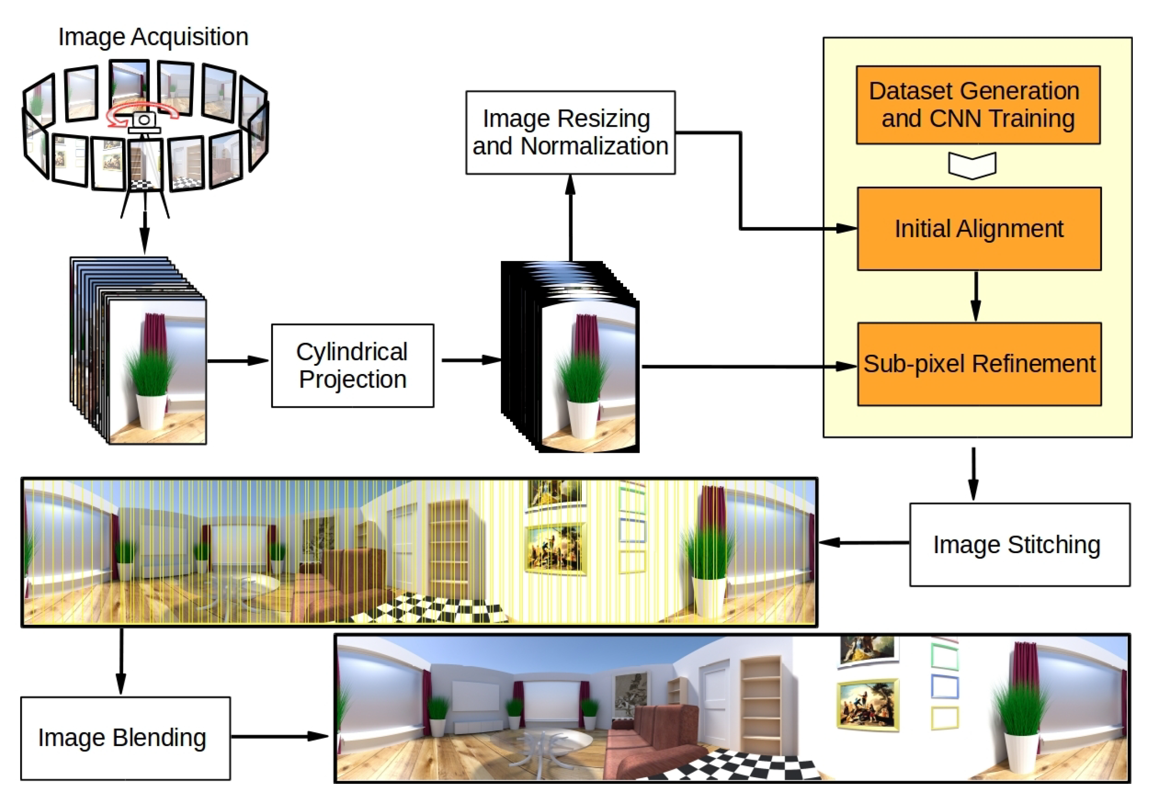
3.1. Overview
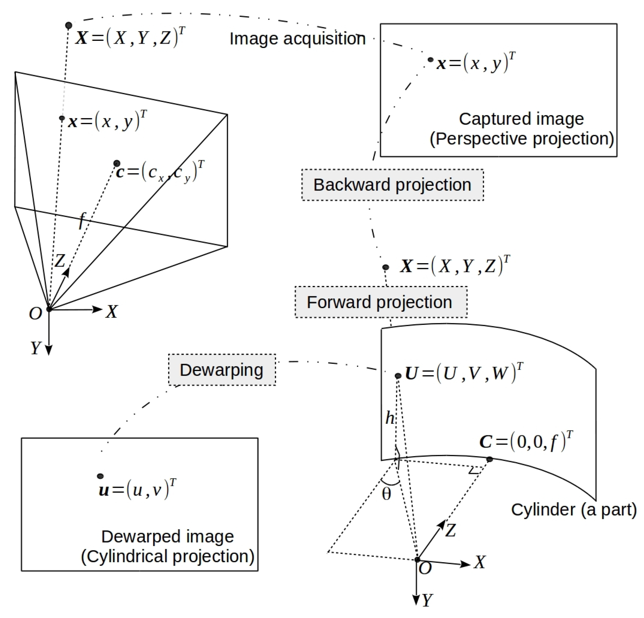
3.2. Cylindrical Projection
3.3. Initial Alignment Using ShiftNet
3.4. Global Illumination Invariant Sub-Pixel Refinement
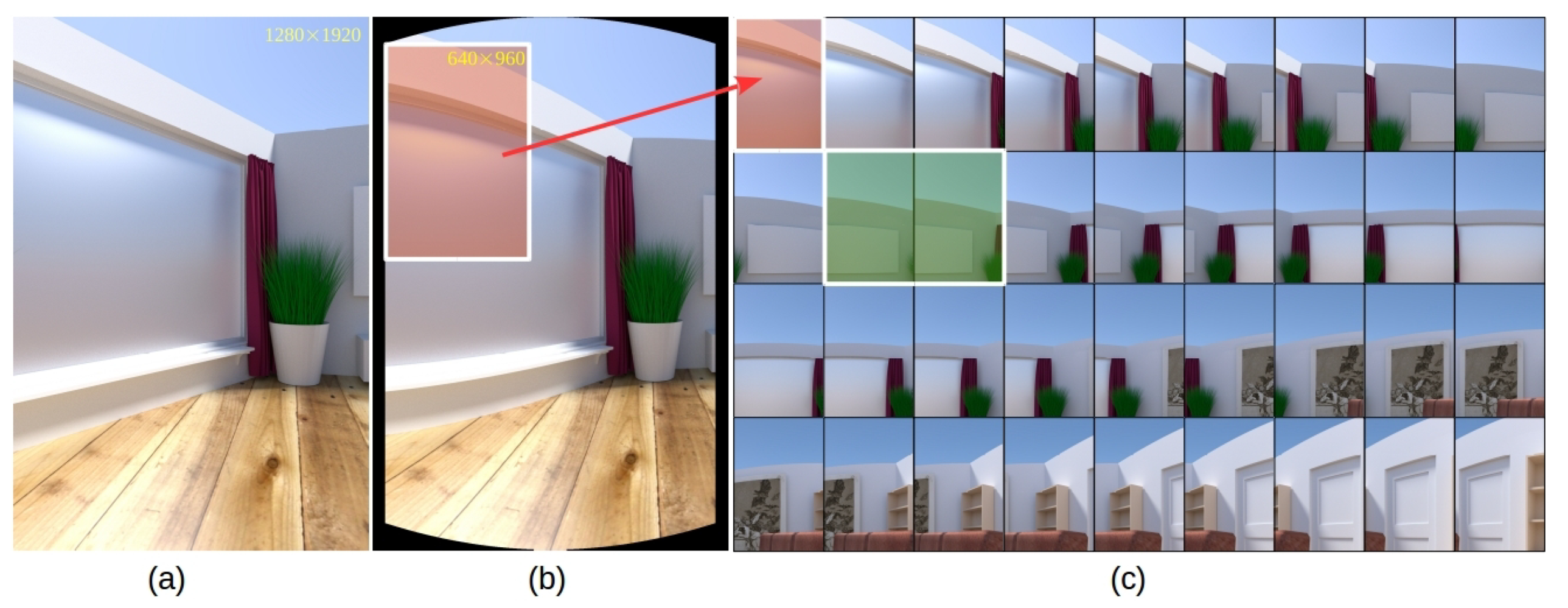
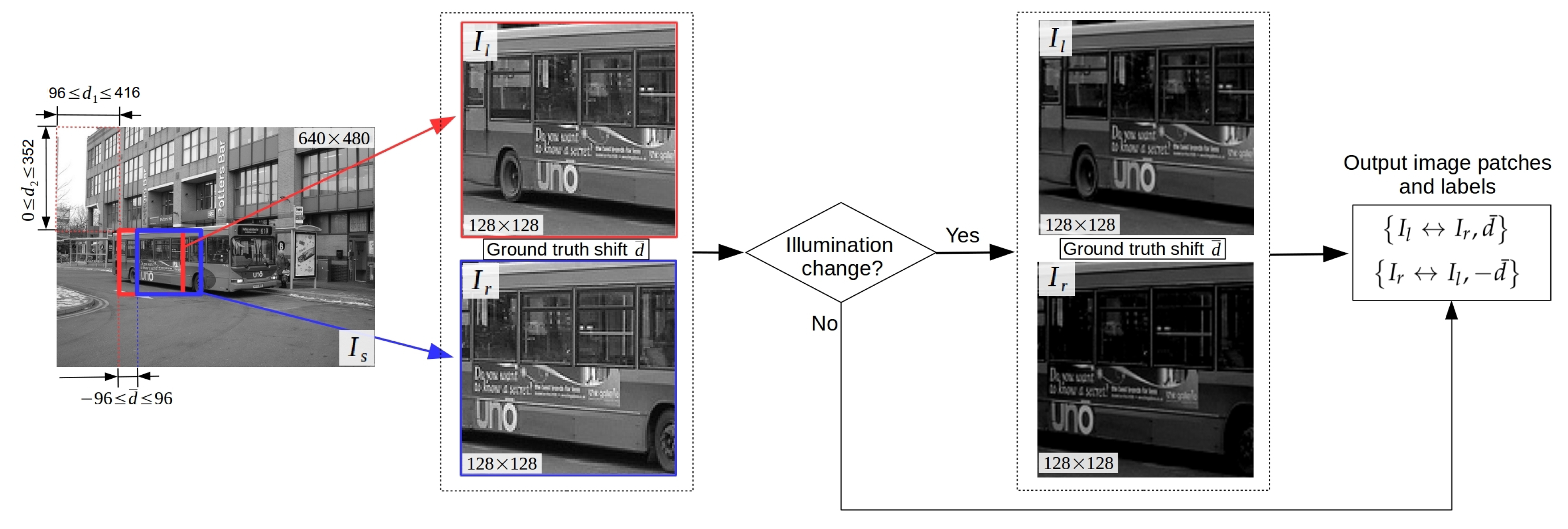
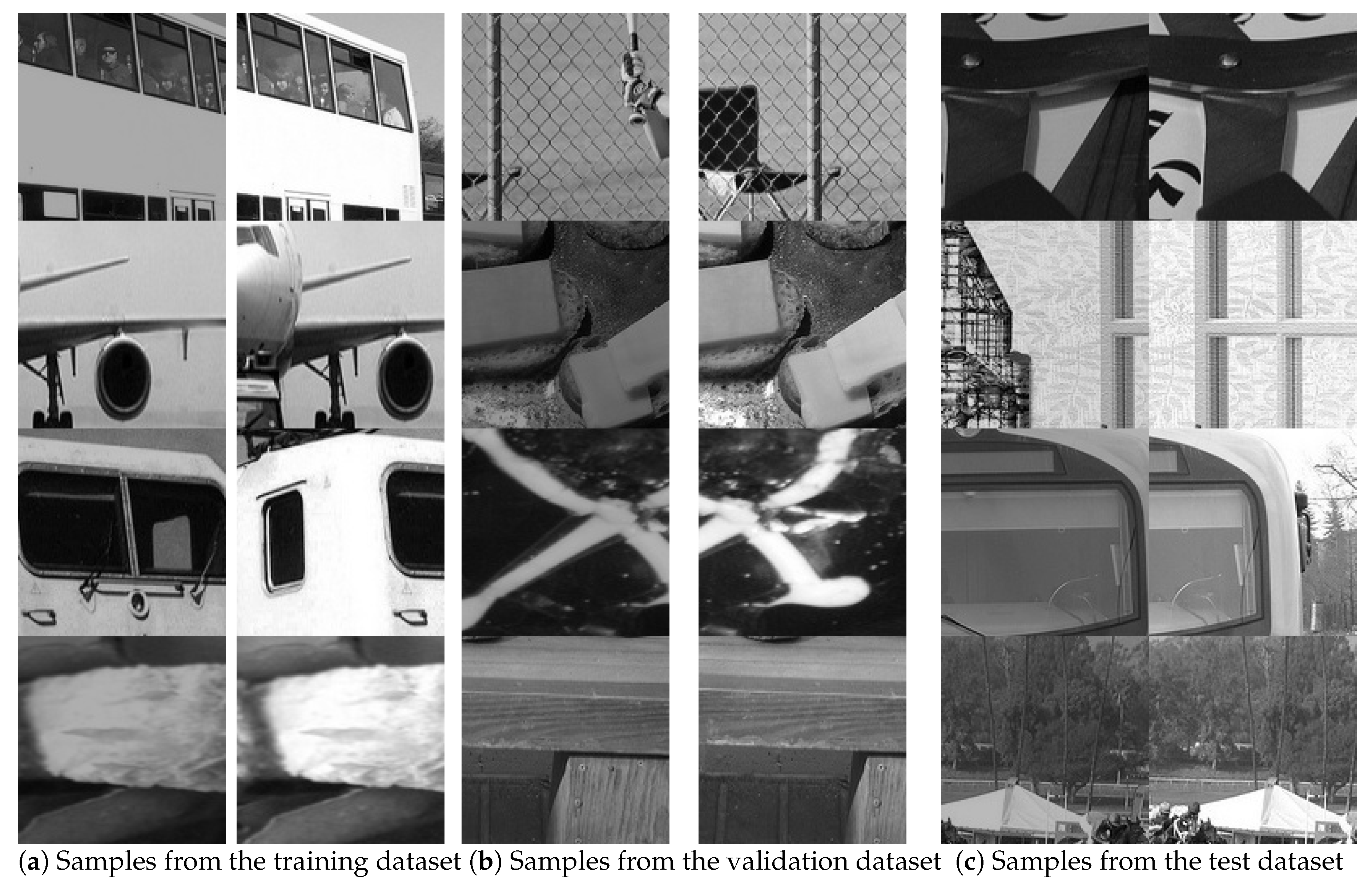
3.5. Synthetic Datasets Generation
4. Experiments
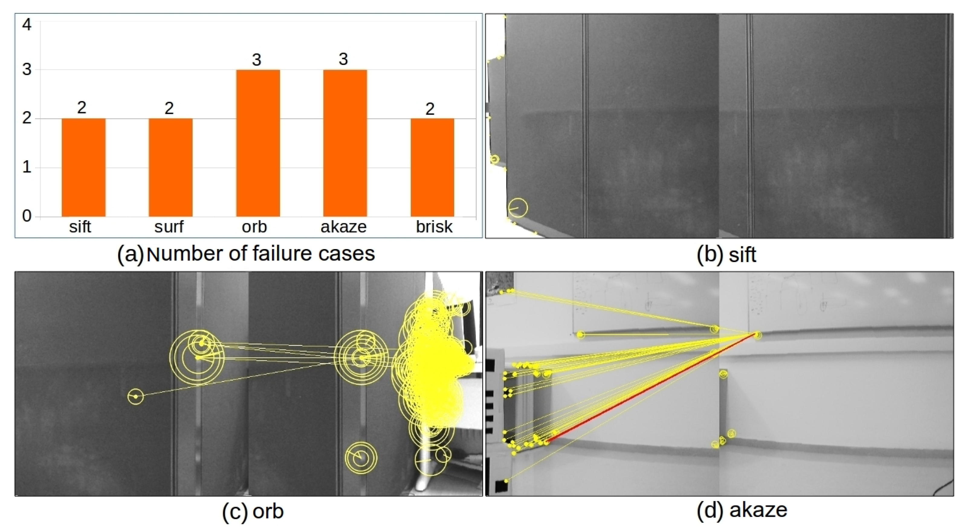
4.1. Baseline Methods
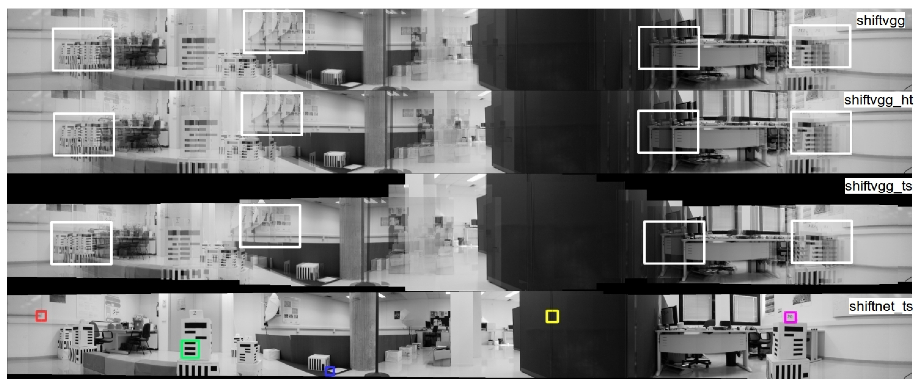
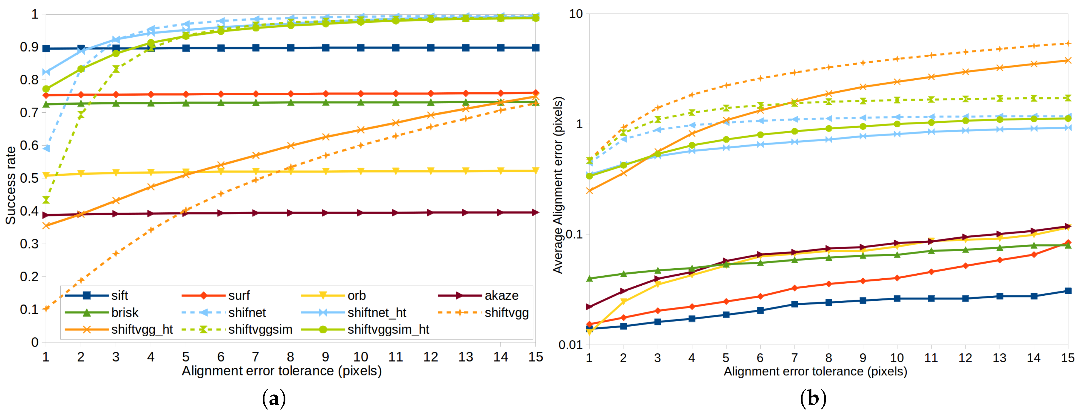
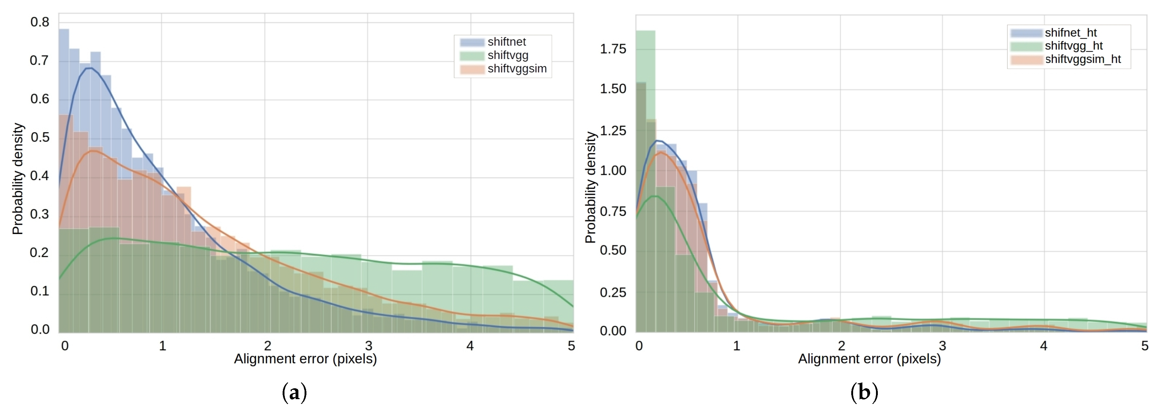
4.2. Experiments on Synthetic Datasets
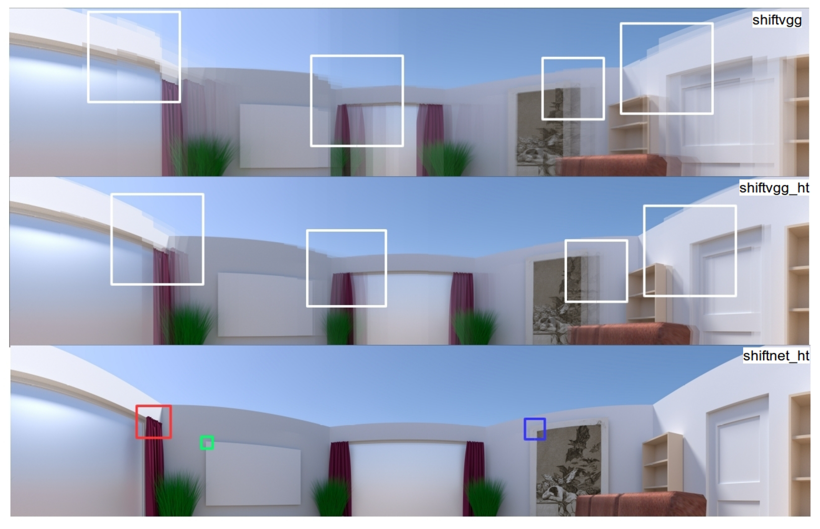
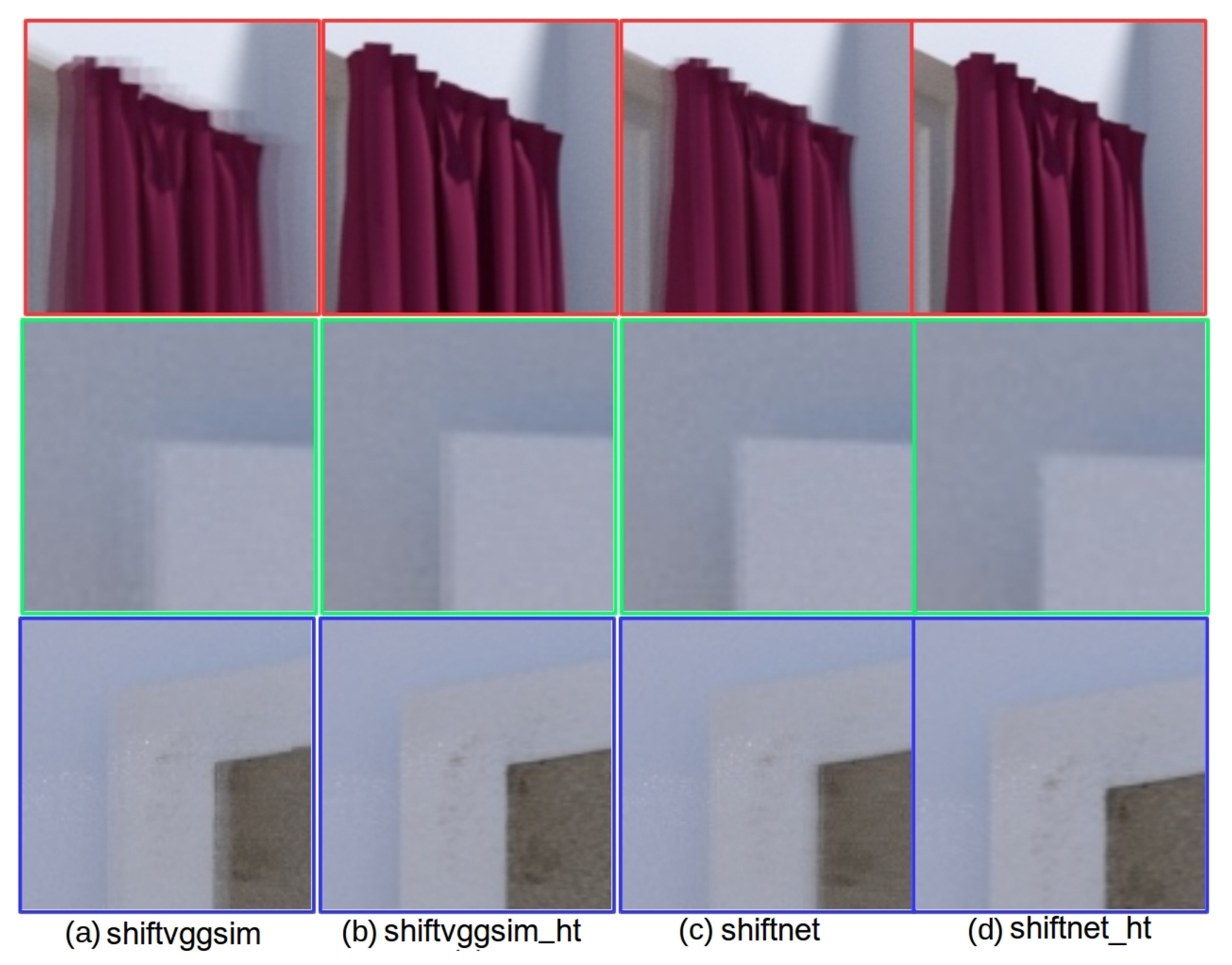
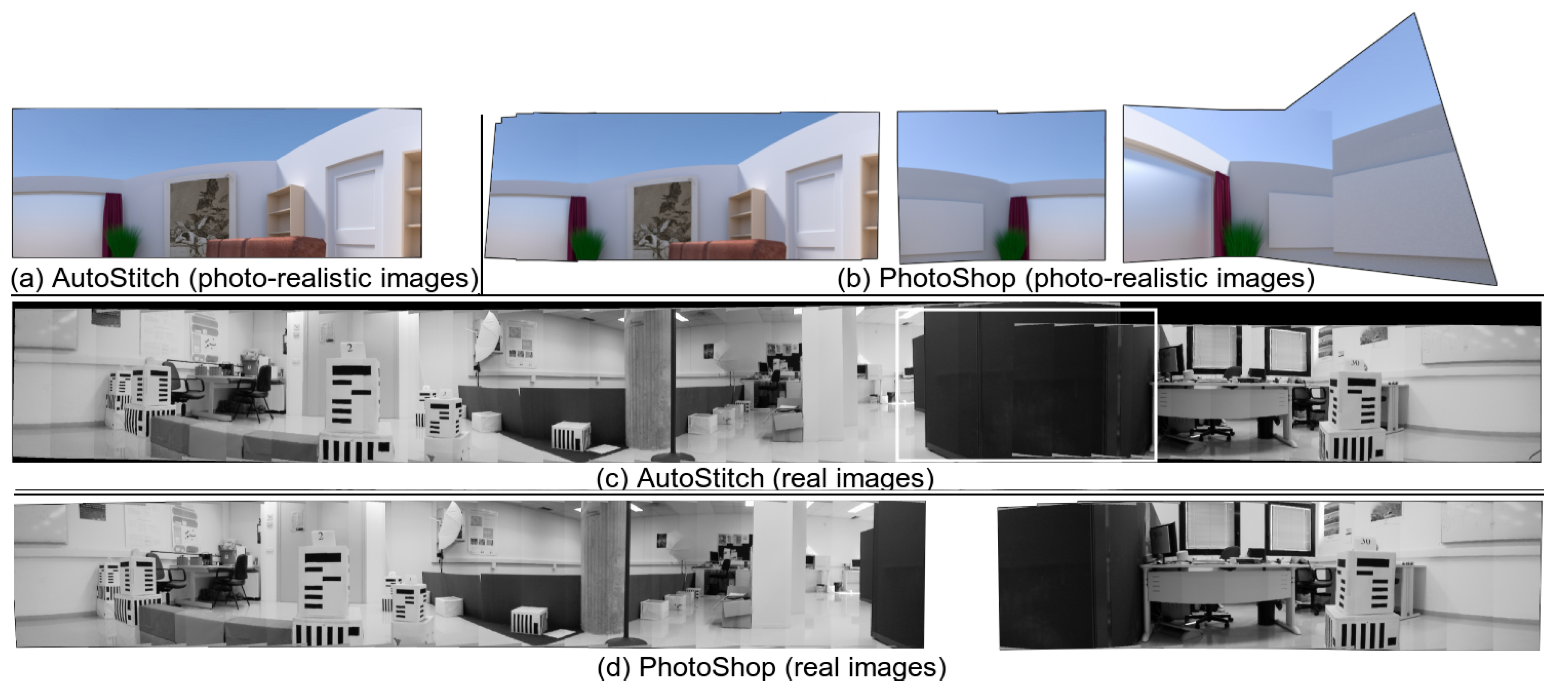
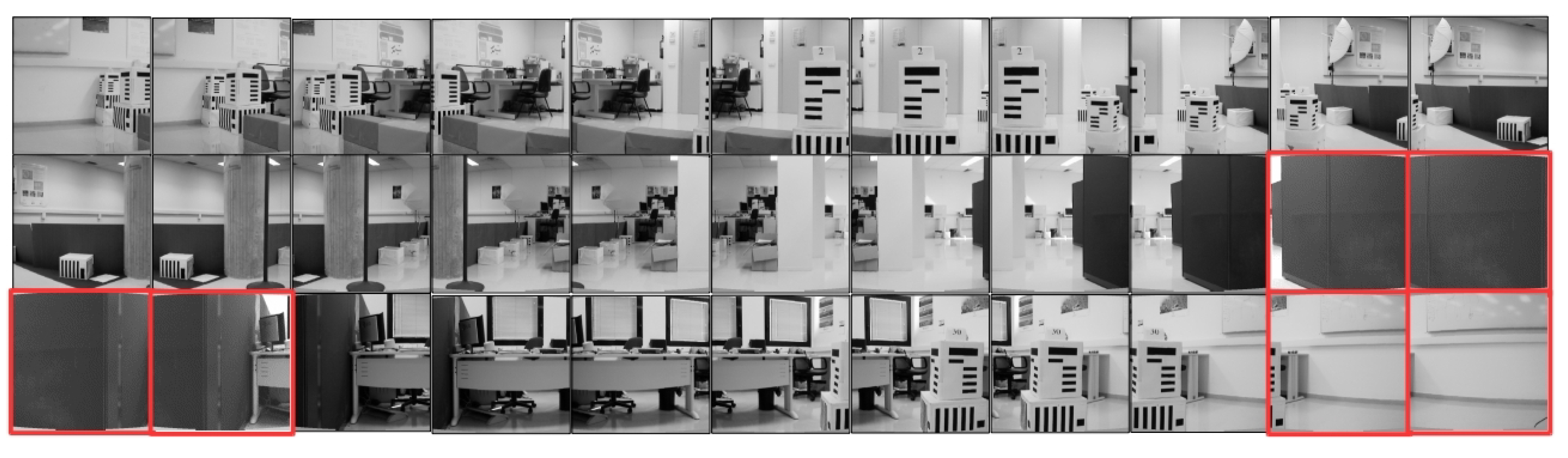
4.3. Experiments on Rendered Photo-Realistic Images
4.4. Experiments on Real Images
4.5. Comparison with Existing Software
5. Conclusions
Author Contributions
Funding
Conflicts of Interest
References
- Yu, M.; Ma, G. 360° Surround View System with Parking Guidance. SAE Int. J. Commer. Veh. 2014, 7, 19–24. [Google Scholar] [CrossRef]
- Scaioni, M.; Barazzetti, L.; Gianinetto, M. Multi-Image Robust Alignment of Medium-Resolution Satellite Imagery. Remote Sens. 2018, 10, 1969. [Google Scholar] [CrossRef]
- Fujita, H.; Mase, M.; Hama, H.; Hasegawa, H. Monitoring Apparatus and Monitoring Method Using Panoramic Image. U.S. Patent Application 10/508,042, 14 January 2004. [Google Scholar]
- Payá, L.; Peidró, L.; Amorós, F.; Valiente, D.; Reinoso, O. Modeling Environments Hierarchically with Omnidirectional Imaging and Global-Appearance Descriptors. Remote Sens. 2018, 10, 522. [Google Scholar] [CrossRef]
- Möller, R.; Vardy, A.; Kreft, S.; Ruwisch, S. Visual Homing in Environments with Anisotropic Landmark Distribution. Auton. Robot. 2007, 23, 231–245. [Google Scholar] [CrossRef]
- Ramisa, R.; Tapus, A.; Mantaras, R.L.; Toledo, R. Mobile Robot Localization using Panoramic Vision and Combinations of Feature Region Detectors. In Proceedings of the 2008 IEEE International Conference on Robotics and Automation, Pasadena, CA, USA, 19–23 May 2008; pp. 538–543. [Google Scholar]
- Yang, K.; Hu, X.; Bergasa, L.M.; Romera, E.; Wang, K. PASS: Panoramic Annular Semantic Segmentation. IEEE Trans. Intell. Transp. Syst. 2019, 1–15. [Google Scholar] [CrossRef]
- Yang, K.; Hu, X.; Chen, H.; Xiang, K.; Wang, K.; Stiefelhagen, R. DS-PASS: Detail-Sensitive Panoramic Annular Semantic Segmentation through SwaftNet for Surrounding Sensing. Available online: https://arxiv.org/pdf/1909.07721.pdf (accessed on 3 November 2019).
- Szeliski, R.; Shum, H.Y. Creating full view panoramic image mosaics and environment maps. In Proceedings of the 24th Annual Conference on Computer Graphics and Interactive Techniques, New York, NY, USA, 3–8 August 1997; pp. 251–258. [Google Scholar]
- Brown, M.; Lowe, D. Automatic Panoramic Image Stitching using Invariant Features. Int. J. Comput. Vis. 2007, 74, 59–73. [Google Scholar] [CrossRef]
- Fischler, M.A.; Bolles, R.C. Random sample consensus: A paradigm for model fitting with applications to image analysis and automated cartography. Commun. ACM 1981, 24, 381–395. [Google Scholar] [CrossRef]
- Lowe, D.G. Distinctive image features from scale-invariant keypoints. Int. J. Comput. Vis. 2004, 60, 91–110. [Google Scholar] [CrossRef]
- Bay, H.; Ess, A.; Tuytelaars, T.; Gool, L.V. Speeded-up robust features (SURF). Comput. Vis. Image Underst. 2008, 110, 346–359. [Google Scholar] [CrossRef]
- Rublee, E.; Rabaud, V.; Konolige, K.; Bradski, G. ORB: An efficient alternative to SIFT or SURF. In Proceedings of the 2011 IEEE International Conference on Computer Vision (ICCV), Barcelona, Spain, 6–13 November 2011; pp. 2564–2571. [Google Scholar]
- Alcantarilla, P.F.; Nuevo, J.; Bartoli, A. Fast Explicit Diffusion for Accelerated Features in Nonlinear Scale Spaces. In Proceedings of the British Machine Vision Conference (BMVC), Bristol, UK, 9–13 September 2013; pp. 13.1–13.11. [Google Scholar]
- Leutenegger, S.; Chli, M.; Siegwart, R.Y. BRISK: Binary robust invariant scalable keypoints. In Proceedings of the 2011 IEEE International Conference on Computer Vision (ICCV), Barcelona, Spain, 6–13 November 2011; pp. 2548–2555. [Google Scholar]
- Lindeberg, T. Scale-space theory: A basic tool for analysing structures at different scales. J. Appl. Stat. 1994, 21, 224–270. [Google Scholar] [CrossRef]
- Rosten, E.; Drummond, T. Machine learning for high-speed corner detection. In Proceedings of the 9th European Conference on Computer Vision (ECCV), Graz, Austria, 7–13 May 2006; pp. 430–443. [Google Scholar]
- Calonder, M.; Lepetit, V.; Strecha, C.; Fua, P. BRIEF: Binary robust independent elementary features. In Proceedings of the 11th European Conference on Computer Vision (ECCV), Heraklion, Crete, Greece, 5–11 September 2010; pp. 778–792. [Google Scholar]
- Alcantarilla, P.F.; Bartoli, A.; Davison, A.J. KAZE features. In Proceedings of the 12th European Conference on Computer Vision (ECCV), Florence, Italy, 7–13 October 2012; pp. 214–227. [Google Scholar]
- Mair, E.; Hager, G.D.; Burschka, D.; Suppa, M.; Hirzinger, G. Adaptive and generic corner detection based on the accelerated segment test. In Proceedings of the 11th European Conference on Computer Vision (ECCV), Heraklion, Crete, Greece, 5–11 September 2010; pp. 183–196. [Google Scholar]
- Tareen, S.A.K.; Saleem, Z. A Comparative Analysis of SIFT, SURF, KAZE, AKAZE, ORB, and BRISK. In Proceedings of the 2018 International Conference on Computing, Mathematics and Engineering Technologies (iCoMET), Sukkur, Pakistan, 3–4 March 2018; pp. 1–10. [Google Scholar]
- Karami, E.; Prasad, S.; Shehata, M. Image Matching Using SIFT, SURF, BRIEF and ORB: Performance Comparison for Distorted Images. In Proceedings of the 2015 Newfoundland Electrical and Computer Engineering Conference, St. John’s, NL, Canada, 5 November 2015. [Google Scholar]
- Xu, Y.; Chen, J.; Liao, T. Ratio-Preserving Half-Cylindrical Warps for Natural Image Stitching. Available online: https://arxiv.org/pdf/1803.06655.pdf (accessed on 3 November 2019).
- Fakour-Sevom, V.; Guldogan, E.; Kamarainen, J.-K. 360 Panorama Super-resolution using Deep Convolutional Networks. In Proceedings of the 13th International Joint Conference on Computer Vision, Imaging and Computer Graphics Theory and Applications (VISIGRAPP 2018), Funchal, Portugal, 27–29 January 2018; pp. 159–165. [Google Scholar]
- Krizhevsky, A.; Sutskever, I.; Hinton, G.E. ImageNet classification with deep convolutional neural networks. In Proceedings of the Advances in Neural Information Processing Systems 25 (NIPS 2012), Lake Tahoe, NV, USA, 3–8 December 2012. [Google Scholar]
- Long, J.; Shelhamer, E.; Darrell, T. Fully convolutional networks for semantic segmentation. In Proceedings of the 2015 IEEE Conference on Computer Vision and Pattern Recognition (CVPR), Boston, MA, USA, 7–12 June 2015; pp. 3431–3440. [Google Scholar]
- Badrinarayanan, V.; Kendall, A.; Cipolla, R. SegNet: A Deep Convolutional Encoder-Decoder Architecture for Image Segmentation. IEEE Trans. Pattern Anal. Mach. Intell. 2017, 39, 2481–2495. [Google Scholar] [CrossRef] [PubMed]
- Girshick, R.; Donahue, J.; Darrell, T.; Malik, J. Rich feature hierarchies for accurate object detection and semantic segmentation. In Proceedings of the 2014 IEEE Conference on Computer Vision and Pattern Recognition (CVPR), Columbus, OH, USA, 23–28 June 2014; pp. 580–587. [Google Scholar]
- Ren, S.; He, K.; Girshick, R.; Sun, J. Faster R-CNN: Towards Real-Time Object Detection with Region Proposal Networks. In Proceedings of the Advances in Neural Information Processing Systems 28 (NIPS 2015), Montreal, QC, Canada, 7–12 December 2015. [Google Scholar]
- DeTone, D.; Malisiewicz, A. Deep Homography Estimation. Available online: https://arxiv.org/abs/1606.03798 (accessed on 13 September 2019).
- Kang, L.; Wei, Y.; Xie, Y.; Jiang, J.; Guo, Y. Combining Convolutional Neural Network and Photometric Refinement for Accurate Homography Estimation. IEEE Access 2019, 7, 109460–109473. [Google Scholar] [CrossRef]
- Ranftl, R.; Koltun, V. Deep Fundamental Matrix Estimation. In Proceedings of the 15th European Conference on Computer Vision (ECCV), Munich, Germany, 8–14 September 2018; pp. 284–299. [Google Scholar]
- Poursaeed, O.; Yang, G.; Prakash, A.; Fang, Q.; Jiang, H.; Hariharan, B.; Belongie, S. Deep Fundamental Matrix Estimation Without Correspondences. In Proceedings of the 15th European Conference on Computer Vision (ECCV) Workshops, Munich, Germany, 8–14 September 2018; pp. 485–497. [Google Scholar]
- Simonyan, K.; Zisserman, A. Very Deep Convolutional Networks for Large-Scale Image Recognition. In Proceedings of the 3rd International Conference on Learning Representations, San Diego, CA, USA, 7–9 May 2015. [Google Scholar]
- Agrawal, P.; Carreira, J.; Malik, J. Learning to see by moving. In Proceedings of the 2015 IEEE International Conference on Computer Vision (ICCV), Santiago, Chile, 7–13 December 2015; pp. 37–45. [Google Scholar]
- Kendall, A.; Grimes, M.; Cipolla, R. PoseNet: A convolutional network for real-time 6-DOF camera relocalization. In Proceedings of the 2015 IEEE International Conference on Computer Vision (ICCV), Santiago, Chile, 7–13 December 2015; pp. 2938–2946. [Google Scholar]
- Kendall, A.; Cipolla, R. Geometric loss functions for camera pose regression with deep learning. In Proceedings of the 2017 IEEE Conference on Computer Vision and Pattern Recognition (CVPR), Honolulu, HI, USA, 21–26 July 2017; pp. 6555–6564. [Google Scholar]
- Ummenhofer, B.; Zhou, H.; Uhrig, J.; Mayer, N.; Ilg, E.; Dosovitskiy, A.; Brox, T. DeMoN: Depth and motion network for learning monocular stereo. In Proceedings of the 2017 IEEE Conference on Computer Vision and Pattern Recognition (CVPR), Honolulu, HI, USA, 21–26 July 2017; pp. 5622–5631. [Google Scholar]
- Meneghetti, G.; Danelljan, M.; Felsber, M.; Nordberg, L. Image alignment for panorama stitching in sparsely structured environments. In Proceedings of the 19th Scandinavian Conference on Image Analysis (SCIA), Copenhagen, Denmark, 15–17 June 2015; pp. 428–439. [Google Scholar]
- Hartley, R.; Zisserman, A. Multiple View Geometry in Computer Vision; Cambridge University Press: New York, NY, USA, 2003. [Google Scholar]
- Lin, T.-Y.; Maire, M.; Belongie, S.; Hays, J.; Perona, P.; Ramanan, D.; Dollár, P.; Zitnick, C.L. Microsoft coco: Common objects in context. In Proceedings of the 13th European Conference on Computer Vision (ECCV), Zurich, Switzerland, 6–12 September 2014; pp. 740–755. [Google Scholar]
- Kingma, D.; Ba, J. Adam: A Method for Stochastic Optimization. Available online: https://arxiv.org/abs/1412.6980 (accessed on 13 September 2019).
- Marron, J.S.; Wand, M.P. Exact Mean Integrated Squared Error. Ann. Stat. 1992, 20, 712–736. [Google Scholar] [CrossRef]


| Methods | Mean | Std. Dev | Median | Minimal | Maximum |
|---|---|---|---|---|---|
| shiftnet | 3.604 | 4.140 | 3.805 | 0.203 | 15.904 |
| shiftnet_ht | 1.517 | 1.531 | 1.274 | 0.090 | 7.487 |
| shiftvgg | 38.236 | 48.473 | 38.947 | 0.210 | 134.098 |
| shiftvgg_ht | 22.473 | 20.354 | 13.504 | 0.027 | 79.191 |
| shiftvggsim | 6.007 | 6.528 | 5.785 | 0.185 | 35.968 |
| shiftvggsim_ht | 6.153 | 2.530 | 1.272 | 0.091 | 35.532 |
© 2019 by the authors. Licensee MDPI, Basel, Switzerland. This article is an open access article distributed under the terms and conditions of the Creative Commons Attribution (CC BY) license (http://creativecommons.org/licenses/by/4.0/).
Share and Cite
Kang, L.; Wei, Y.; Jiang, J.; Xie, Y. Robust Cylindrical Panorama Stitching for Low-Texture Scenes Based on Image Alignment Using Deep Learning and Iterative Optimization. Sensors 2019, 19, 5310. https://doi.org/10.3390/s19235310
Kang L, Wei Y, Jiang J, Xie Y. Robust Cylindrical Panorama Stitching for Low-Texture Scenes Based on Image Alignment Using Deep Learning and Iterative Optimization. Sensors. 2019; 19(23):5310. https://doi.org/10.3390/s19235310
Chicago/Turabian StyleKang, Lai, Yingmei Wei, Jie Jiang, and Yuxiang Xie. 2019. "Robust Cylindrical Panorama Stitching for Low-Texture Scenes Based on Image Alignment Using Deep Learning and Iterative Optimization" Sensors 19, no. 23: 5310. https://doi.org/10.3390/s19235310
APA StyleKang, L., Wei, Y., Jiang, J., & Xie, Y. (2019). Robust Cylindrical Panorama Stitching for Low-Texture Scenes Based on Image Alignment Using Deep Learning and Iterative Optimization. Sensors, 19(23), 5310. https://doi.org/10.3390/s19235310