Data Uploading Strategy for Underwater Wireless Sensor Networks

Abstract
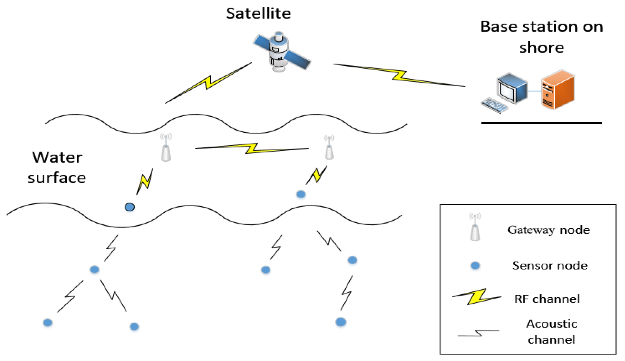
:1. Introduction
2. Related Work
2.1. Data Reduction Strategies in UWSNs
2.2. Data Reduction Strategies in WSNs
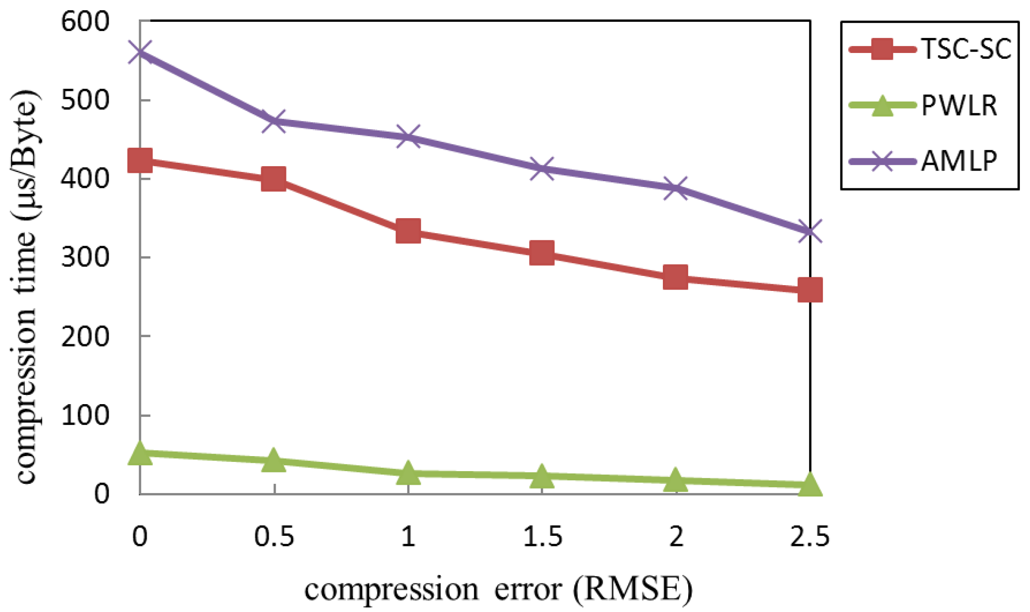
2.3. Temporal Domain Compression Algorithms
2.4. Spatial Compression Algorithm
2.5. Spatial-Temporal Domain Compression Algorithm
3. Data Uploading Strategy
3.1. Relevant Concepts
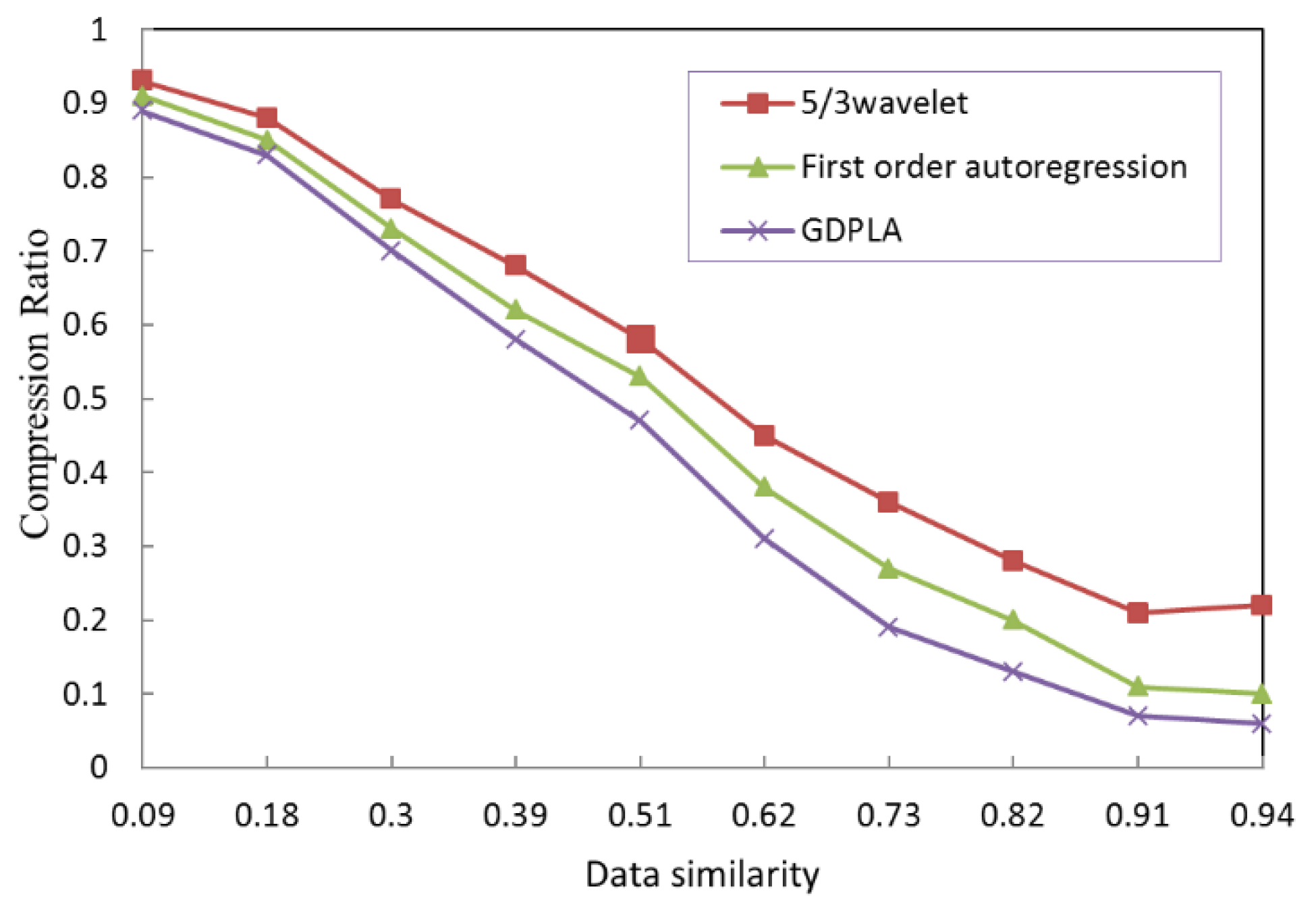
3.1.1. Compression Ratio (CR)
3.1.2. Data Similarity
- (1)
- When the overlapping ratio in each dimension remains unchanged, the greater the intersecting dimensionality, the higher the similarity.
- (2)
- When the intersecting dimensionality between data sets remains unchanged, the larger the overlapping ratio in each dimension, the higher the similarity.
3.2. Joint Power Control and Rate Adaptation Algorithm
3.2.1. Power Control Algorithm
Sharing Mode
Exclusive Mode
3.2.2. Rate Adaptation Algorithm
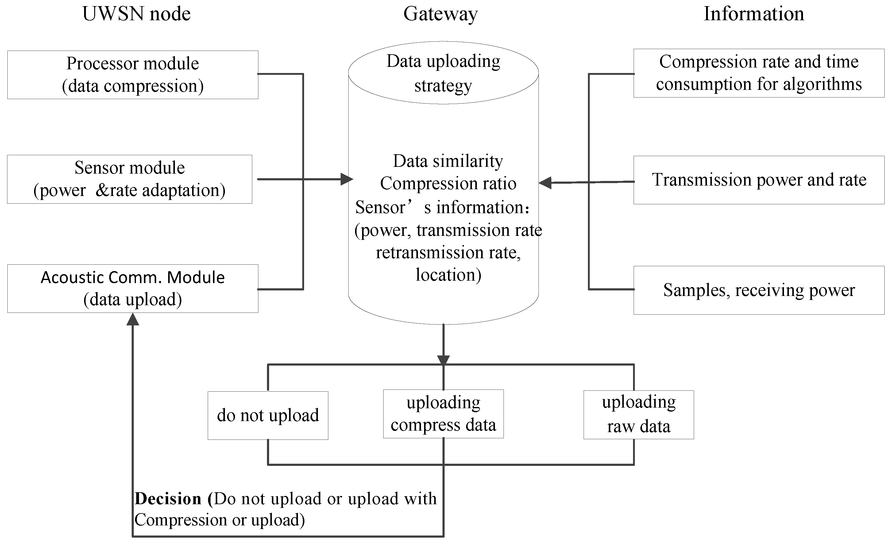
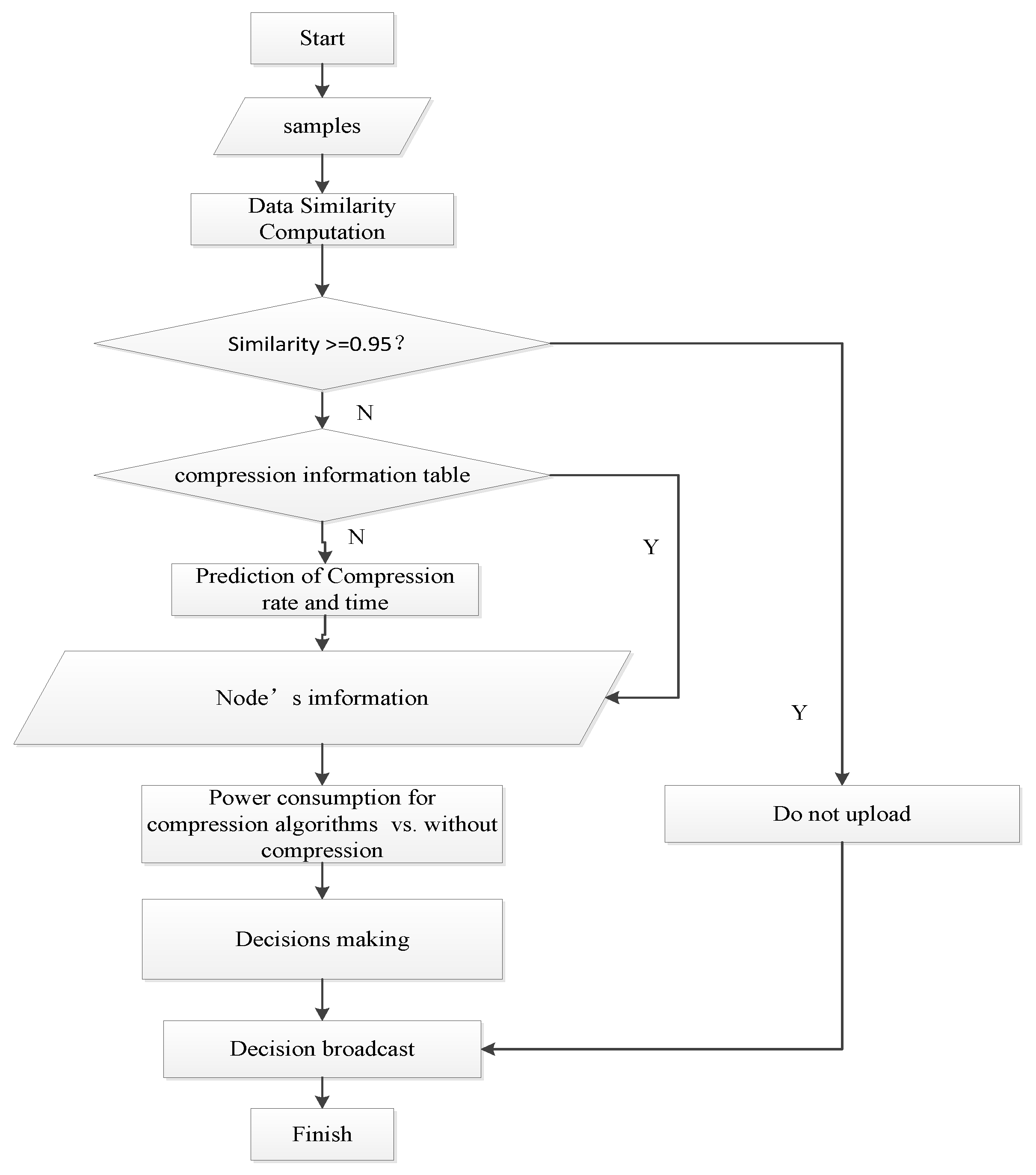
3.3. Data Upload Decision-Making Mechanism
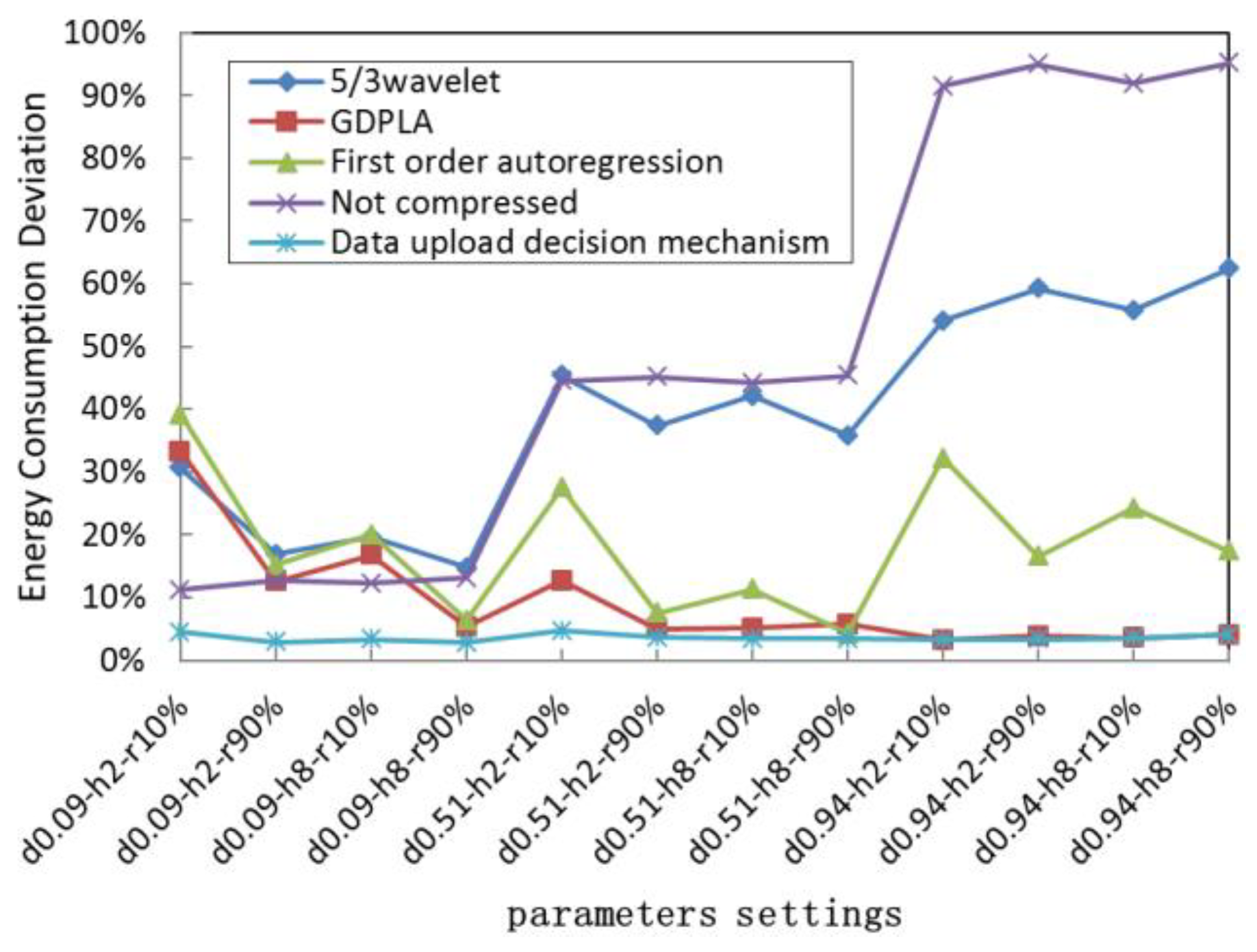
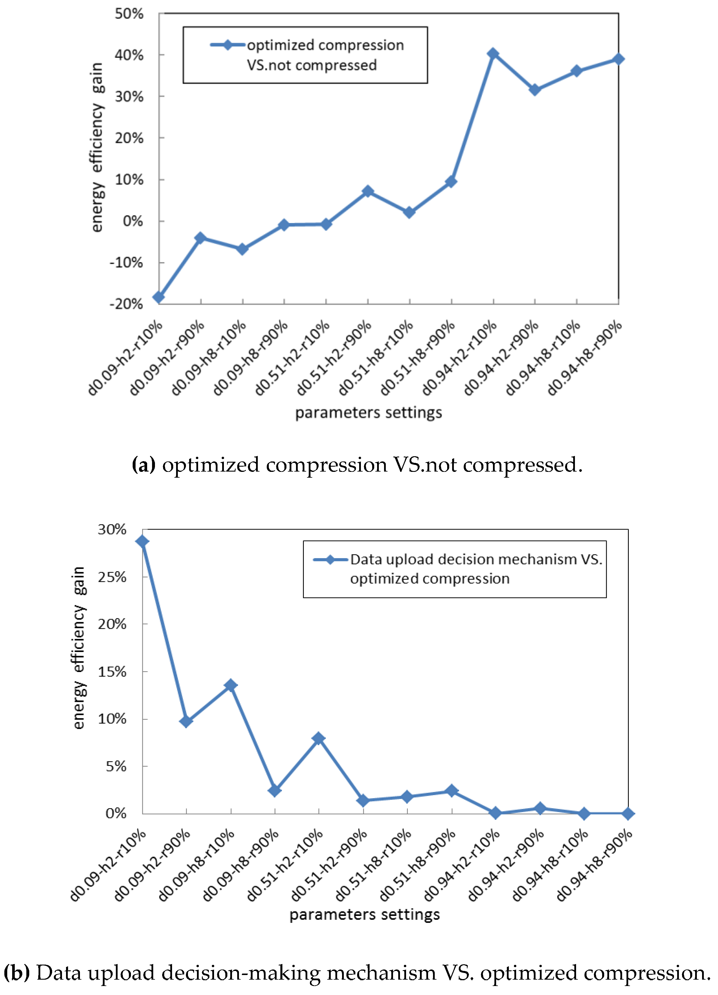
4. Simulation and Evaluation
5. Conclusions
Author Contributions
Funding
Conflicts of Interest
References
- Wan, L.; Zhou, H.; Xu, X.; Huang, Y.; Zhou, S.; Shi, Z.; Cui, J.H. Field tests of adaptive modulation and coding for underwater acoustic OFDM. IEEE J. Ocean. Eng. 2015, 40, 327–336. [Google Scholar] [CrossRef]
- Lin, J.W.; Liao, S.W.; Leu, F.Y. Sensor Data Compression Using Bounded Error Piecewise Linear Approximation with Resolution Reduction. Energies 2019, 12, 2523. [Google Scholar] [CrossRef]
- Zhu, L. Research on WSN Data Compression Based on Predictive Class Aglorithm. Master’s Thesis, Taiyuan University of Technology, Taiyuan, China, 2018; pp. 49–53. [Google Scholar]
- Shuang, Z.; Zhihong, Q.; Xiaohui, L. Data Compression Algorithm Based on Sequence Correlation for WSN. J. Electron. Inf. Technol. 2016, 38, 713–719. [Google Scholar]
- Chen, S.; Lu, J. An Adaptive Multiple-Modality Sensor Network Data Compression Algorithm Based on Lifting Wavelet and Polynomial Fitting. Chin. J. Sens. Actuators 2013, 26, 550–557. [Google Scholar]
- Zhang, R.; Du, S.; Chen, L.; Kan, J.; Xu, G. Data Compression Method with Piece-Wise Linear Regression in WSN. Chin. J. Sens. Actuators 2015, 28, 531–536. [Google Scholar]
- Atmel Corporation. AVR Studio 4. [2009-05-16]. Available online: http://www.atmel.com/dyn/Products/tools_card.asp?tool_id=2725 (accessed on 16 May 2009).
- Li, C.; Wang, J.; Li, M. An Efficient Cross-Layer Optimization Algorithm for Data Transmission in Wireless Sensor Networks. Int. J. Wirel. Inf. Netw. 2017, 24, 462–469. [Google Scholar] [CrossRef]
- Adcock, B.; Hansen, A.C. Generalized sampling and infinite-dimensional compressed sensing. F Found. Comput. Math. 2016, 16, 1263–1323. [Google Scholar] [CrossRef]
- Jianhua, Q.; Xueying, Z. Compressed sensing based data gathering in wireless sensor networks: A survey. J. Comput. Appl. 2017, 37, 3261–3269. [Google Scholar]
- Liu, B.; Zhang, Z. Quantized Compressive Sensing for Low-Power Data Compression and Wireless Telemonitoring. IEEE Sens. J. 2016, 16, 8206–8213. [Google Scholar] [CrossRef]
- Lin, H.; Wei, W.; Zhao, P.; Ma, X.; Zhang, R.; Liu, W.; Deng, T.; Peng, K. Energy-efficient compressed data aggregation in underwater acoustic sensor networks. Wirel. Netw. 2016, 22, 1985–1997. [Google Scholar] [CrossRef]
- Wang, D.; Xu, R.; Hu, X.; Su, W. Energy-Efficient Distributed Compressed Sensing Data Aggregation for Cluster-Based Underwater Acoustic Sensor Networks. Int. J. Distrib. Sens. Netw. 2016, 2016, 19. [Google Scholar] [CrossRef]
- Jing, L.; He, C.; Huang, J.; Ding, Z. Energy Management and Power Allocation for Underwater Acoustic Sensor Network. IEEE Sens. J. 2017, 17, 6451–6462. [Google Scholar] [CrossRef]
- Liu, G.; Kang, W. IDMA-Based Compressed Sensing for Ocean Monitoring Information Acquisition with Sensor Networks. Math. Probl. Eng. 2014, 2014, 1–13. [Google Scholar] [CrossRef]
- Wu, F.Y.; Yang, K.; Duan, R.; Tian, T. Compressive Sampling and Reconstruction of Acoustic Signal in Underwater Wireless Sensor Networks. IEEE Sens. J. 2018, 18, 5876–5884. [Google Scholar] [CrossRef]
- Li, S.; Kim, J.G.; Han, D.H.; Lee, K.S. A Survey of Energy-Efficient Communication Protocols with QoS Guarantees in Wireless Multimedia Sensor Networks. Sensors 2019, 19, 199. [Google Scholar] [CrossRef]
- Taherpour, A.; Chobin, M.; Rahmani, M. Collaborative data aggregation using multiple antennas sensors and fusion centre with energy harvesting capability in WSN. IET Commun. 2019, 13, 1971–1979. [Google Scholar]
- Rane, S.; Cohen, R.A.; Vetro, A.; Sugimoto, K. Method for Improving Compression Efficiency of Distributed Source Coding Using Intra-Band Information. U.S. Patent 9,307,257 B2, 26 March 2015. [Google Scholar]
- Diallo, O.; Rodrigues, J.J.P.C.; Sene, M.; Lloret, J. Distributed Database Management Techniques for Wireless Sensor Networks. IEEE Trans. Parallel Distrib. Syst. 2015, 26, 604–620. [Google Scholar] [CrossRef]
- Diallo, O.; Rodrigues, J.J.; Sene, M.; Lloret, J. Simulation framework for real-time database on WSNs. J. Netw. Comput. Appl. 2014, 39, 191–201. [Google Scholar] [CrossRef]
- Bonnet, P.; Gehrke, J.; Seshadri, P. Towards Sensor Database Systems. In Proceedings of the International Conference on Mobile Data Management, Hong Kong, China, 8–10 January 2001; Springer-Verlag: London, UK, 2001; pp. 3–14. [Google Scholar]
- Umar, M.M.; Khan, S.; Ahmad, R.; Singh, D. Game Theoretic Reward Based Adaptive Data Communication in Wireless Sensor Networks. IEEE Access 2018, 6, 28073–28084. [Google Scholar] [CrossRef]
- Hu, H.; He, J.; Wu, J.; Wang, K.; Zhuang, W. Distributed high-dimensional similarity search approach for large-scale wireless sensor networks. Int. J. Distrib. Sens. Netw. 2017, 13, 1–10. [Google Scholar] [CrossRef]
- Lazaridis, I.; Mehrotra, S. Capturing sensor-generated time series with quality guarantees. In Proceedings of the 19th International Conference on Data Engineering (Cat. No.03CH37405), Bangalore, India, 5–8 March 2003; IEEE: Piscataway, NJ, USA, 2003; pp. 429–440. [Google Scholar]
- Yan, H.; Shi, Z.; Cui, J.H. DBR: Depth-Based Routing for Underwater Sensor Network. In Proceedings of the 2018 International Conference on Research in Networking, Singapore, 5–9 May 2008; pp. 72–86. [Google Scholar]
- Pham, M.L.; Ramstad, T.A.; Balasingham, I. Ultra wideband biomedical wireless sensor networks using wavelet lifting for image transmission. In Proceedings of the 2009 International Conference on Information Processing in Sensor Networks, San Francisco, CA, USA, 13–16 April 2009; IEEE Computer Society: Washington, DC, USA, 2009; pp. 385–386. [Google Scholar]
- Wang, L.; Ma, C. A one-dimensional linear regression model based spatial and temporal data compression algorithm for wireless senor networks. J. Electron. Inf. Technol. 2010, 32, 755–758. [Google Scholar] [CrossRef]
- Elmeleegy, H.; Elmagarmid, A.K.; Cecchet, E.; Aref, W.G.; Zwaenepoel, W. Online piece-wise linear approximation of numerical streams with precision guarantees. VLDB Endow. 2009, 2, 145–156. [Google Scholar] [CrossRef]
- Yu, L.; Li, J.; Gao, H.; Fang, X. Enabling ε-Approximate Querying in Sensor Network. Proc. VLDB Endow. 2009, 2, 169–180. [Google Scholar] [CrossRef]
- Fazel, F.; Fazel, M.; Stojanovic, M. Random access compressed sensing for energy-efficient underwater sensor networks. IEEE J. Sel. Areas Commun. 2011, 29, 1660–1670. [Google Scholar] [CrossRef]
- Siripanadorn, S.; Hattagam, W.; Teaumroong, N. Anomaly detection in wireless sensor networks using self-organizing map and wavelets. Int. J. Commun. 2010, 4, 74–83. [Google Scholar]
- Pattem, S.; Krishnamachari, B.; Govindan, R. The impact of spatial correlation on routing with compression in wireless sensor networks. ACM Trans. Sens. Netw. 2008, 4, 24. [Google Scholar] [CrossRef]
- Kolo, J.G.; Ang, L.M.; Shanmugam, S.A.; Lim, D.W.G.; Seng, K.P. A Simple Data Compression Algorithm for Wireless Sensor Networks. In Soft Computing Models in Industrial and Environmental Applications; Springer: Berlin, Germany, 2013; pp. 327–336. [Google Scholar]
- Zhou, S.W.; Lan, L.I. DTW-based multi-wavelet data compression algorithm for wireless sensor networks. J. Commun. 2014, 35, 86–94. [Google Scholar]
- Zhu, T.J.; Lin, Y.P.; Zhou, S.W.; Xu, X.L. Adaptive multiple-modalities data compression algorithm using wavelet for wireless sensor networks. J. Commun. 2009, 30, 48–53. [Google Scholar]
- Luo, C.; Wu, F.; Sun, J.; Chen, C.W. Compressive data gathering for large-scale wireless sensor networks. In Proceedings of the 15th Annual International Conference on Mobile Computing and Networking, Beijing, China, 20–25 September 2009; ACM: New York, NY, USA, 2009; pp. 145–156. [Google Scholar]
- Jiang, P.; Wu, J.F.; Wu, B.; Dong, L.X.; Wang, D. Data compression method for wireless sensor networks based on adaptive optimal zero suppression. J. Commun. 2013, 34, 1–7. [Google Scholar]
- Chen, Z.; Yang, G.; Chen, L.; Zhou, Q. Data gathering for long network lifetime in WSNs based on compressed sensing. J. Electron. Inf. Technol. 2014, 36, 2343–2349. [Google Scholar]
- Ji, J.; Pang, W.; Zhou, C. A fuzzy k-prototype clustering algorithm for mixed numeric and categorical data. Knowl. Based Syst. 2012, 30, 129–135. [Google Scholar] [CrossRef]
- Wu, X.; Chen, G. Avoiding energy holes in wireless sensor networks with non-uniform node distribution. IEEE Trans. Parallel Distrib. Syst. 2018, 19, 710–720. [Google Scholar]
- Pottier, A.; Socheleau, F.X.; Laot, C. Power-efficient spectrum sharing for noncooperative underwater acoustic communication systems. In Proceedings of the OCEANS 2016 MTS/IEEE Monterey, Monterey, CA, USA, 19–23 September 2016; IEEE: Piscataway, NJ, USA, 2016; pp. 1–6. [Google Scholar]
- Yao, G.; Jin, Z.; Su, Y. An environment-friendly spectrum decision strategy for underwater wireless sensor networks. In Proceedings of the 2015 IEEE International Conference on Communications, London, UK, 8–12 June 2015; pp. 6370–6375. [Google Scholar]
- Caspers, E.P.; Yeung, S.H.; Sarkar, T.K. Analysis of Information and Power Transfer in Wireless Communications. IEEE Antennas Propag. Mag. 2013, 55, 82–95. [Google Scholar] [CrossRef]
- Janik, V.M. Source levels and the estimated active space of bottlenose dolphin (Tursiops truncatus) whistles in the Moray Firth, Scotland. J. Comp. Physiol. A 2000, 186, 673–680. [Google Scholar] [CrossRef] [PubMed]
- Yan, H.; Zhou, S.; Shi, Z.J.; Li, B. A DSP implementation of OFDM acoustic modem. In Proceedings of the Second Workshop on Underwater Networks, Montreal, QC, Canada, 14 September 2007; pp. 89–92. [Google Scholar]
- Li, J.; Li, G.; Gao, H. Novel E-Approximation to Data Streams in Sensor Networks. IEEE Trans. Parallel Distrib. Syst. 2015, 26, 1654–1667. [Google Scholar] [CrossRef]
- Zhang, Y.; Chen, H.; Xu, W.; Yang, T.C.; Huang, J. Spatiotemporal Tracking of Ocean Current Field with Distributed Acoustic Sensor Network. IEEE J. Ocean. Eng. 2017, 42, 681–696. [Google Scholar] [CrossRef]
- Ding, L.; Chen, W. The Analysis and Research of Lifting Scheme based on Wavelet Transform. In Proceedings of the International Conference on Cyber Security Intelligence and Analytics, Shenyang, China, 21–22 February 2019; pp. 1377–1382. [Google Scholar]
- Cao, B.; Zhao, J.; Lv, Z.; Liu, X.; Kang, X.; Yang, S. Deployment optimization for 3D industrial wireless sensor networks based on particle swarm optimizers with distributed parallelism. J. Netw. Comput. Appl. 2018, 103, 225–238. [Google Scholar] [CrossRef]


| Data Rate (kbps) | 1–10 |
|---|---|
| Processing power (W) | <0.8 |
| Transmission power (W) | <35 |
| Data similarity | 0.09 | 0.18 | 0.30 | 0.39 | 0.51 | 0.62 | 0.73 | 0.82 | 0.91 | 0.94 |
| 5/3 wavelet | 0.93 | 0.88 | 0.77 | 0.68 | 0.58 | 0.45 | 0.36 | 0.28 | 0.21 | 0.22 |
| First-order autoregression | 0.91 | 0.85 | 0.73 | 0.62 | 0.53 | 0.38 | 0.27 | 0.20 | 0.11 | 0.10 |
| GDPLA | 0.89 | 0.83 | 0.70 | 0.58 | 0.47 | 0.31 | 0.19 | 0.13 | 0.07 | 0.06 |
| Compression Accuracy | No. Hops | Retransmission Ratio | 5/3 Wavelet | GDPLA | First-Order Autoregression | Not Compressed | Data Upload Decision-Making Mechanism |
|---|---|---|---|---|---|---|---|
| 0.09 | 2 | 10% | 30.67% | 33.25% | 39.18% | 11.26% | 4.51% |
| 0.09 | 2 | 90% | 16.89% | 12.57% | 15.24% | 12.66% | 2.89% |
| 0.09 | 8 | 10% | 19.62% | 16.81% | 20.03% | 12.29% | 3.31% |
| 0.09 | 8 | 90% | 14.82% | 5.27% | 6.41% | 13.11% | 2.85% |
| 0.51 | 2 | 10% | 45.36% | 12.64% | 27.48% | 44.52% | 4.71% |
| 0.51 | 2 | 90% | 37.34% | 4.97% | 7.56% | 45.18% | 3.59% |
| 0.51 | 8 | 10% | 42.07% | 5.16% | 11.34% | 44.19% | 3.38% |
| 0.51 | 8 | 90% | 35.84% | 5.79% | 4.26% | 45.34% | 3.41% |
| 0.94 | 2 | 10% | 54.11% | 3.23% | 32.16% | 91.46% | 3.21% |
| 0.94 | 2 | 90% | 59.24% | 3.86% | 16.59% | 94.92% | 3.32% |
| 0.94 | 8 | 10% | 55.78% | 3.51% | 24.27% | 91.89% | 3.51% |
| 0.94 | 8 | 90% | 62.32% | 4.02% | 17.39% | 95.16% | 4.01% |
© 2019 by the authors. Licensee MDPI, Basel, Switzerland. This article is an open access article distributed under the terms and conditions of the Creative Commons Attribution (CC BY) license (http://creativecommons.org/licenses/by/4.0/).
Share and Cite
Huang, X.; Sun, S.; Yang, Q. Data Uploading Strategy for Underwater Wireless Sensor Networks. Sensors 2019, 19, 5265. https://doi.org/10.3390/s19235265
Huang X, Sun S, Yang Q. Data Uploading Strategy for Underwater Wireless Sensor Networks. Sensors. 2019; 19(23):5265. https://doi.org/10.3390/s19235265
Chicago/Turabian StyleHuang, Xiangdang, Shijie Sun, and Qiuling Yang. 2019. "Data Uploading Strategy for Underwater Wireless Sensor Networks" Sensors 19, no. 23: 5265. https://doi.org/10.3390/s19235265
APA StyleHuang, X., Sun, S., & Yang, Q. (2019). Data Uploading Strategy for Underwater Wireless Sensor Networks. Sensors, 19(23), 5265. https://doi.org/10.3390/s19235265