1. Introduction
Recent social advancements and rapid industrialization have led to concerns about climate change and the ever-increasing demand for energy, which is a recognized problem of international significance. The World Energy Outlook Report [
1] indicates that global energy demand is set to grow by 90% by 2040. The need for the efficient use of energy resources and reduced carbon footprints has led to a systematic deployment of cyber–physical systems (CPS) such as smart grid [
2]. A smart grid enables the distribution and consumption of energy resources in a more efficient, effective and economical way. Smart meters are now an integral part of advanced metering infrastructure (AMI) of a smart grid that allows appliance load monitoring (ALM) [
3] to enable real-time energy consumption reporting and feedback.
Non-intrusive load monitoring (NILM) is a process of estimating the energy consumption of the appliances in a consumer’s (e.g., household or industry) premises. NILM is a non-intrusive technique that estimates appliance-level energy consumption based on the aggregated power consumption readings gathered from a consumer’s smart meter [
3]. NILM also enables real-time monitoring and feedback on the end-user’s appliance consumption. It also allows utilities to perform real-time load analysis and more accurate energy forecasting, which saves them operational time and expense. This feedback gives the consumer insight into the amount of energy an appliance consumes to help make informed decisions about conserving power, whether motivated by economic or ecologic concerns (or both). Research findings suggest that residential appliance-level power usage feedback results in savings of up to 12% of annual power consumption [
4]. Feedback also improves awareness of one’s behavior. The more closely electricity consumption can be linked to specific appliances and activities, the clearer the relevance of the behavior becomes. Detailed appliance-specific feedback i.e., the operational state can help a consumer determine as to how a certain appliance behaves and its effect on electricity consumption whether economic or ecological. This also increases the sense of control because the consumer can find out how changes in behavior or appliance operation can affect the outcome [
5].
Research in NILM has made advances in integrating a combination of signal processing, statistical and machine learning technologies to provide a cost-effective approach for load forecasting [
6], real-time monitoring, and feedback [
7]. However, one of the key issues is to accurately evaluate and report the performance of existing NILM approaches. Recent research findings [
8,
9] on NILM algorithms and their implementation conclude that there are some practical limitations of the existing metrics: first, existing event classification metrics do not classify multi-state devices accurately with respect to events in the original ground truth; second, although the overall energy of a device is estimated, it does not measure the energy estimation of each classified state of the device; finally, with relatively large errors the metric result exceeds the usual accuracy interval of 0 and 1, making it less intuitive and explainable.
This paper solves these problems by proposing multi-state energy classifier (MEC) which is a new metric based on unsupervised clustering technique that combines event classification and energy estimation by identifying the operational states of the device from a labeled dataset to compute a penalty threshold for predictions that are too far away from the ground truth. We evaluate our approach using the widely accepted NILMKTK [
10] framework and various publicly available datasets such as the Reference Energy Disaggregation dataset (REDD) [
11], Dutch Residential Energy dataset (DRED) [
12] and Almanac of Minutely Power dataset (AMPds) [
13].
1.1. Motivation and Related Works
NILM takes the aggregate power readings from a smart meter and predicts power levels and device states for every appliance connected to the smart meter.
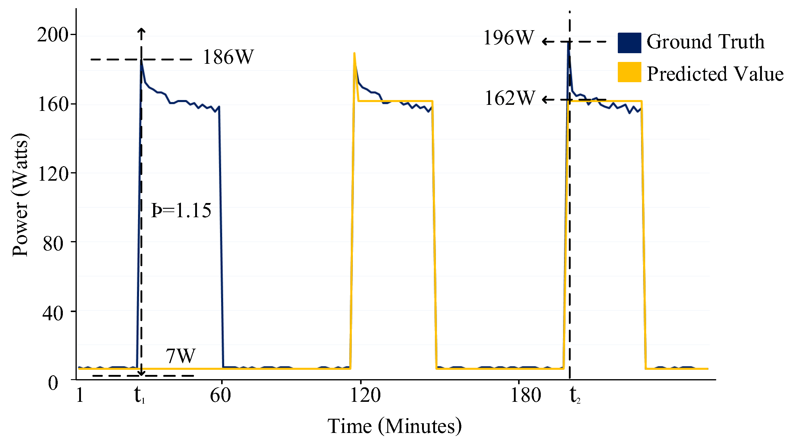
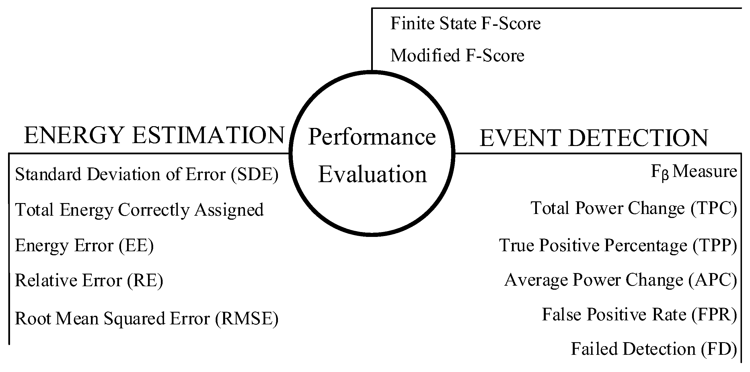
Figure 1 presents the ground truth power signal pattern (blue) and the disaggregated output (yellow) of a NILM algorithm for the fridge. Although NILM techniques have been applied widely for real-time monitoring and energy consumption feedback, the accurate evaluation of NILM approaches has been a critical issue, especially for multi-state devices. An accurate evaluation of different operational states of a multi-state device can help the consumer gain valuable insight as to how a certain appliance behaves, its operational efficiency and the effect on electricity consumption. Several performance metrics have been proposed and used by researchers to evaluate NILM algorithms.
Tsai et al. [
14] and Chang et al. [
15] used the concept of recognition accuracy, which works at a very high sampling rate (e.g., 1
s to 100 ms) to match patterns. However, these techniques cannot be directly applied to smart-meter-based power disaggregation since smart meters report data at a much lower sampling rate (e.g., 1 s up to 10 min based on utility settings). Batra et al. [
16] used root mean square error (RMSE) as one of the energy estimation accuracy metrics. RMSE measures how spread out the predicted values are from their ground truth. The measure is not normalized which makes it difficult to compare the disaggregation accuracy between different appliances. The normalized disaggregation error (NDE) [
17] metric addresses the normalization issue of RMSE. However, NDE tends to report inflated accuracy.
Kolter et al. [
11] proposed total energy correctly assigned (TECA), a method to report estimation accuracies. However, the metric tends to report inflated accuracies. As shown in
Figure 1, a fridge has the ground-truth value of 186W (compressor ON-state) and an estimated value of 7W (compressor off-state) for a given time period
. The TECA metric reported accuracy of 51% for time
. Huang et al. [
18] and Osathanunkul et al. [
19] used the information retrieval domain metric F1-score to evaluate the performance of the energy disaggregation approaches for different sampling rates. The information retrieval domain metric F-score does not differentiate between the multiple operational states of an appliance.
Kim et al. [
20] presented a modified F-score (M-Fscore) which combines the appliance state classification and power estimation accuracies together. The MF-score applies a threshold of standard deviation by the mean to divide the true positive (TP) into accurate true positive (ATP) and inaccurate true positive (ITP) for the appliance. However, the MF-score does not consider the multistate characteristic of an appliance.
As shown in
Figure 1, suppose we have an appliance (fridge) with
of 82.31 and a
of 70.99, then the threshold
is 1.15. For a given time period
, the ground truth value of the fridge is 186 W (compressor on-state) and the estimated value is 7 W (compressor off-state). The higher threshold
resulted in classifying this event as an ATP which would result in an inaccurate increase in reporting NILM accuracy.
Makonin et al. [
21] proposed Finite-state F-score (FS-FScore) to calculate the accuracy of a non-binary classification. A partial penalization measure called an inaccurate portion of true-positive (inacc) was introduced to convert the binary nature of TP into a discrete measure. There are two problems associated with FS-Score. First, the calculation of inacc requires the knowledge of pre-defined states of an appliance. Second, while the FS F-score differentiates between multiple states, it does not correctly consider the measurement variations within the same operational state. For example, for a given time period
in
Figure 1, the ground truth value of the fridge is 196 W and the estimated value is 162 W. Clearly, the metric does not penalize the algorithm for such a large variation.
1.2. Contribution
In this paper, we propose a novel performance evaluation metric multi-state energy classifier (MEC) which can be used to accurately measure the performance of the NILM algorithms, yielding the following contributions:
the proposed metric accurately classifies the operational states of an appliance of different categories with respect to events in the original ground truth;
the proposed metric combines energy estimation with event classification to accurately quantify and penalize the algorithm with respect to variation in the measurements of the state of an appliance;
evaluation and implementation of two state-of-the-art NILM approaches and their performance with several existing and proposed evaluation metrics (see
Section 4);
The paper is organized as follows. In
Section 2, we briefly discuss the technological concepts used in this work. In
Section 3, we present the proposed metric and perform classification and estimation testing in
Section 4 on real-world publicly available datasets. We look at why researchers need to report accuracy with respect to both event classification and energy estimation and conclude the paper in
Section 5.
3. Proposed Metric
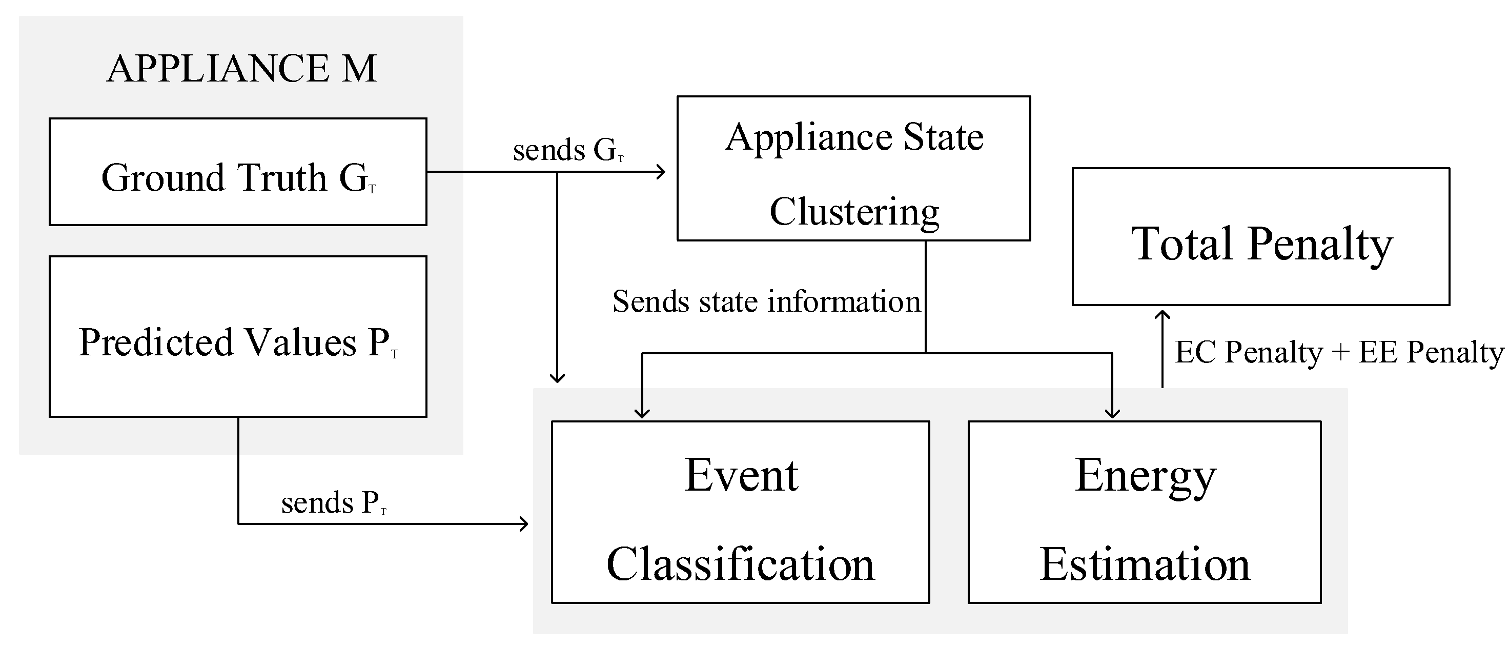
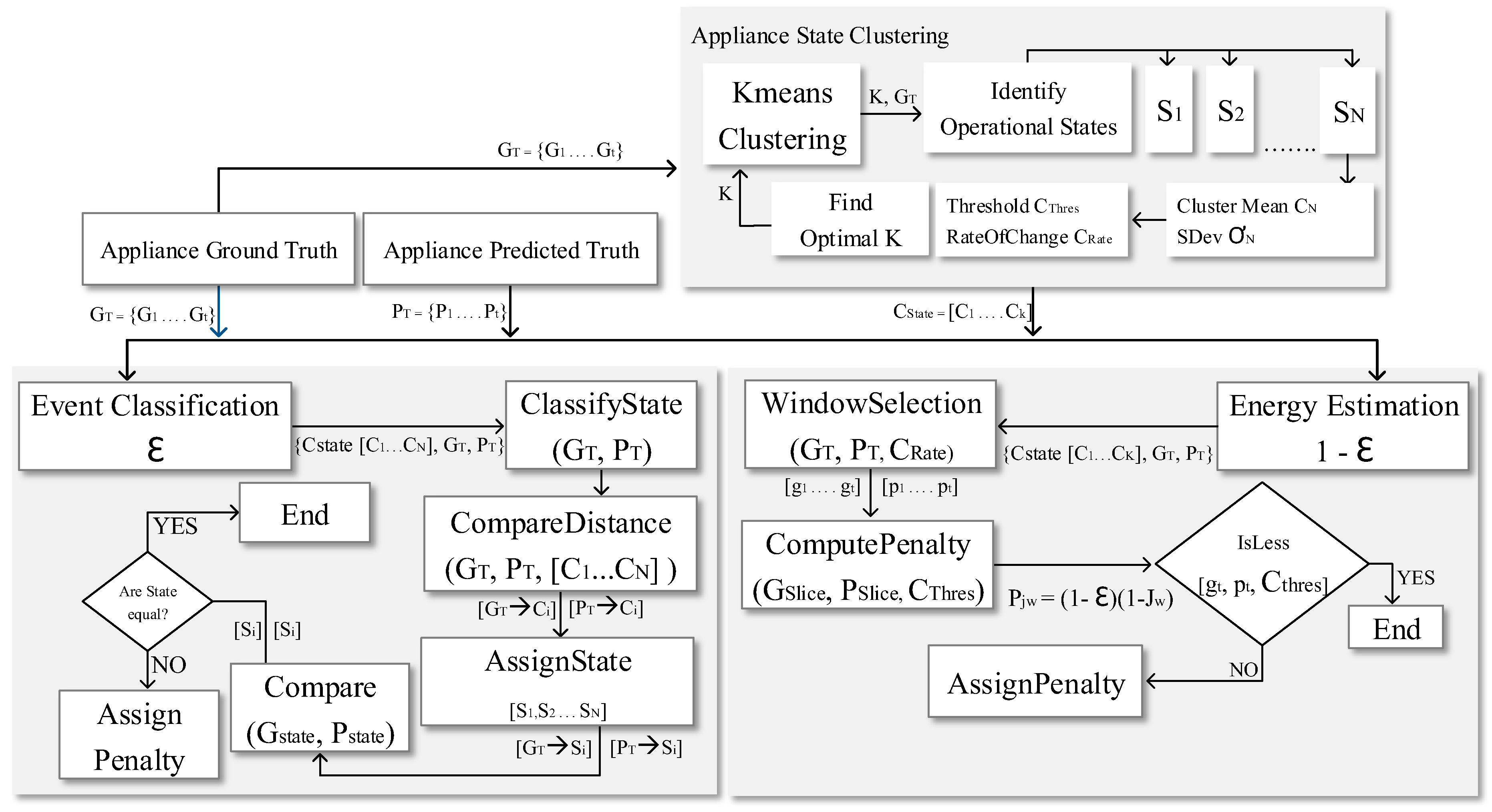
This section presents the MEC metric, as shown in
Figure 5.
Figure 5 illustrates the overall MEC process which comprises three important steps: appliance state clustering; event classification penalty; and energy estimation penalty.
Algorithm 1 describes the process depicted in
Figure 5. Line 1 of Algorithm 1 identifies the operational states of the appliance. The operational states compute the required parameters and the threshold to accurately penalize misclassification or incorrect energy estimation. We apply the penalty for inaccurate event classification in line 2. Next, we penalize the incorrect energy estimation in line 3. The total penalty for incorrect event classification and inaccurate energy estimation is computed in line 4.
| Algorithm 1 Multi-state energy classifier (MEC). |
Input:
is the ground truth of appliance m
is the predicted values of appliance m
= Accuracy weightage for event classification
= Accuracy weightage for energy estimation
Output:
= MEC accuracy for appliance m- 1:
= - 2:
= (,,) - 3:
= (,,) - 4:
= + - 5:
return
|
The total penalty is divided into two parts: event classification penalty and energy estimation penalty. A user-supplied parameter
enables the users to assign more or less weight to either type of penalty according to their requirement. The total penalty is the weighted sum of the individual penalties (Equation (
4)). The three key processes of the MEC metric are presented in detail in the following subsections and also presented in
Figure 6.
3.1. Appliance State Clustering
The appliance state clustering process identifies different clusters that relate to the different operational states of an appliance. To improve the performance of event classification and energy estimation, the usage of the clustering scheme is an important factor. In this paper, we use the k-means algorithm for clustering the operational states of the appliance based on the ground truth data available in the NILM dataset.
To determine the number of clusters, we use the elbow method with k-means clustering.
Once the number of clusters is determined, the k-means clustering algorithm is applied to the appliance ground truth. Based on the unlabelled clustering results, we identify the different operational states of an appliance. Furthermore, we compute the parameters related to the operational state of the appliances as shown in Algorithm 2 which will be used by Algorithms 3 and 4.
| Algorithm 2 Appliance state clustering. |
Input:
is the ground truth of appliance m
N = Maximum number of states
Output:
is the clustered operational states of appliance m- 1:
Standardize the values of time series - 2:
fortoNdo - 3:
Compute within groups sum of squares (WSS) - 4:
end for - 5:
Obtain K using elbow method - 6:
Perform K-Means clustering on to find K clusters - 7:
where - 8:
fortoKdo - 9:
Get and of cluster - 10:
- 11:
where - 12:
Store in - 13:
Store in - 14:
end for - 15:
return
|
3.2. Event Classification Penalty
As explained in
Section 1.1, the existing metrics often overestimate the accuracy of a NILM algorithm due to the incorrect classification of multiple states of an appliance. Algorithm 3 quantifies the inaccuracy of an event that has been misclassified by the NILM algorithm and applies a penalty based on the appliance states computed in Algorithm 2. Algorithm 3 describes the process depicted in
Figure 6 in detail.
| Algorithm 3 Event classification penalty (ECPenalty). |
Input:
is the ground truth of appliance m
is the predicted values of appliance m
is the clustered operational state data of appliance m
Output:
is the total Event Classification Penalty for appliance m- 1:
Set - 2:
fortoTdo - 3:
Get datapoint and - 4:
if and then - 5:
Compute closestCluster - 6:
Set state of to - 7:
Compute closestCluster - 8:
Set state of to - 9:
end if - 10:
if state of then - 11:
Set penalty equal to 1 - 12:
else - 13:
Set penalty equal to 0 - 14:
end if - 15:
end for - 16:
return
|
The input for Algorithm 3 is the operational states information (output from Algorithm 2), the ground truth and the predicted values of a NILM algorithm for appliance m. Next, in Line 3, Algorithm 3 takes the data points , that correspond to the TP output from an NILM algorithm. For a True Positive prediction of a NILM, refers to the ground truth value while refers to its corresponding predicted value. Lines 5–8 obtain the clusters (obtained from Algorithm 2) closest to the data points (, ) and matches the states of the assigned clusters in Lines 6 and 8. Lines 10–14 assign a penalty if the states of corresponding data points , do not match. We define as the total penalty for the inaccurate classification of operational state. The energy estimation penalty is explained next.
3.3. Energy Estimation Penalty
The energy estimation penalty process quantifies the inaccuracy of the estimated energy using an NILM algorithm. Algorithm 4 describes the process depicted in
Figure 6 in detail.
| Algorithm 4 Energy estimation penalty (EEPenalty) |
Input:
is the ground truth of appliance m
is the predicted values of appliance m
is the clustered operational state data of appliance m
is a vector of all
is a vector of all
Output:
is the total Energy estimation Penalty for appliance m- 1:
Init - 2:
fortoTdo - 3:
Obtain data point and - 4:
if and then - 5:
Compute closestCluster - 6:
Compute closestCluster - 7:
Obtain and - 8:
Set and - 9:
while ( and ) do - 10:
Add data point to - 11:
Add data point to - 12:
Increment l - 13:
end while - 14:
Set - 15:
Call ComputePenalty() - 16:
Call AssignPenalty() - 17:
end if - 18:
end for - 19:
return - 20:
- 21:
Procedure ComputePenalty - 22:
Compute - 23:
Compute - 24:
EndProcedure - 25:
- 26:
Procedure AssignPenalty - 27:
fortoldo - 28:
if then - 29:
Assign penalty - 30:
else - 31:
Assign penalty - 32:
end if - 33:
end for - 34:
EndProcedure
|
Algorithm 4 takes the operational states information (output from Algorithm 2), the ground truth and the predicted values of an appliance as an input to provide a penalty for an inaccurate estimation . Similar to the event classification penalty process, we implement Algorithm 4 for all the predicted TP values from an NILM algorithm. The energy estimation penalty process is subdivided into three steps:
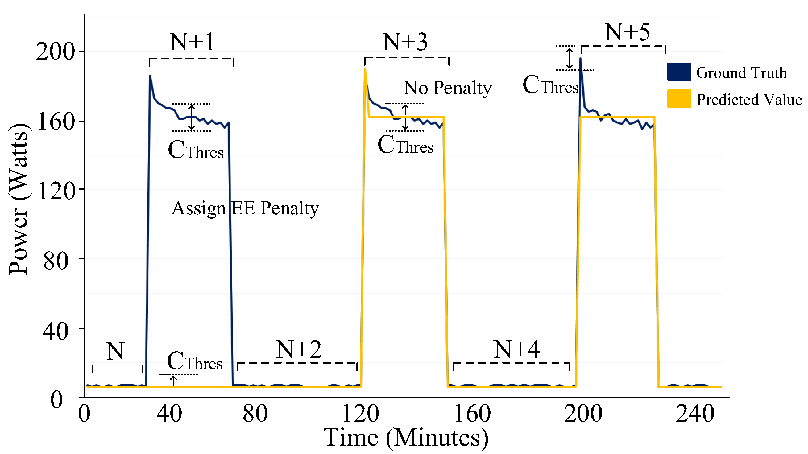
Step 1—window selection: in the window selection process, the basic idea of Algorithm 4 is to divide the time series values of ground truth and the corresponding predicted values into windows, based on changes in the power consumption that reflect a change in the operational state of an appliance as shown in Figure 9. The algorithm starts by traversing through the data points of the ground truth time series and the predicted value time series . The operational states of the starting data points and are determined by assigning the data points to their closest clusters and for the ground truth and the predicted values, respectively. Next, to check if the following points i.e., and belong to the same state, line 10 checks the rate of change of power using and . The and are thresholds for the clusters to which and belong to. The threshold is defined as , where represents 99.7% probability that the points belong to that cluster.
While traversing through the time series, if Algorithm 4 detects a rate of change in either of the time series and , it marks the end of the same operational state and stores them in and respectively (lines 10–11). The traversing process in this step ensures that; firstly and only contain true positives; secondly, the data points in and belong to the same operational state as their members respectively.
Step 2—computing energy estimation penalty: the next step in Algorithm 4 involves calculating the penalty for the and . In line 15, Algorithm 4 calls the procedure defined in Line 21–26. Next, the procedure calculates the penalty in Line 24, where is .
Step 3—assigning energy estimation penalty: the third step of Algorithm 4 is to assign the penalty computed in the previous step. In line 31, Algorithm 4 assigns the penalty to all the true postive values of the window that have predicted values too far from the ground truth as defined by line 28 , where ensures that the predicted values far from the clustered operational state are penalized. is defined as , where and is the standard deviation and mean of the cluster, the ground truth data point belongs to.
4. Implementation and Results
The MEC is implemented on the disaggregation results of two NILM algorithms: FHMM [
20] and SparseViterbi [
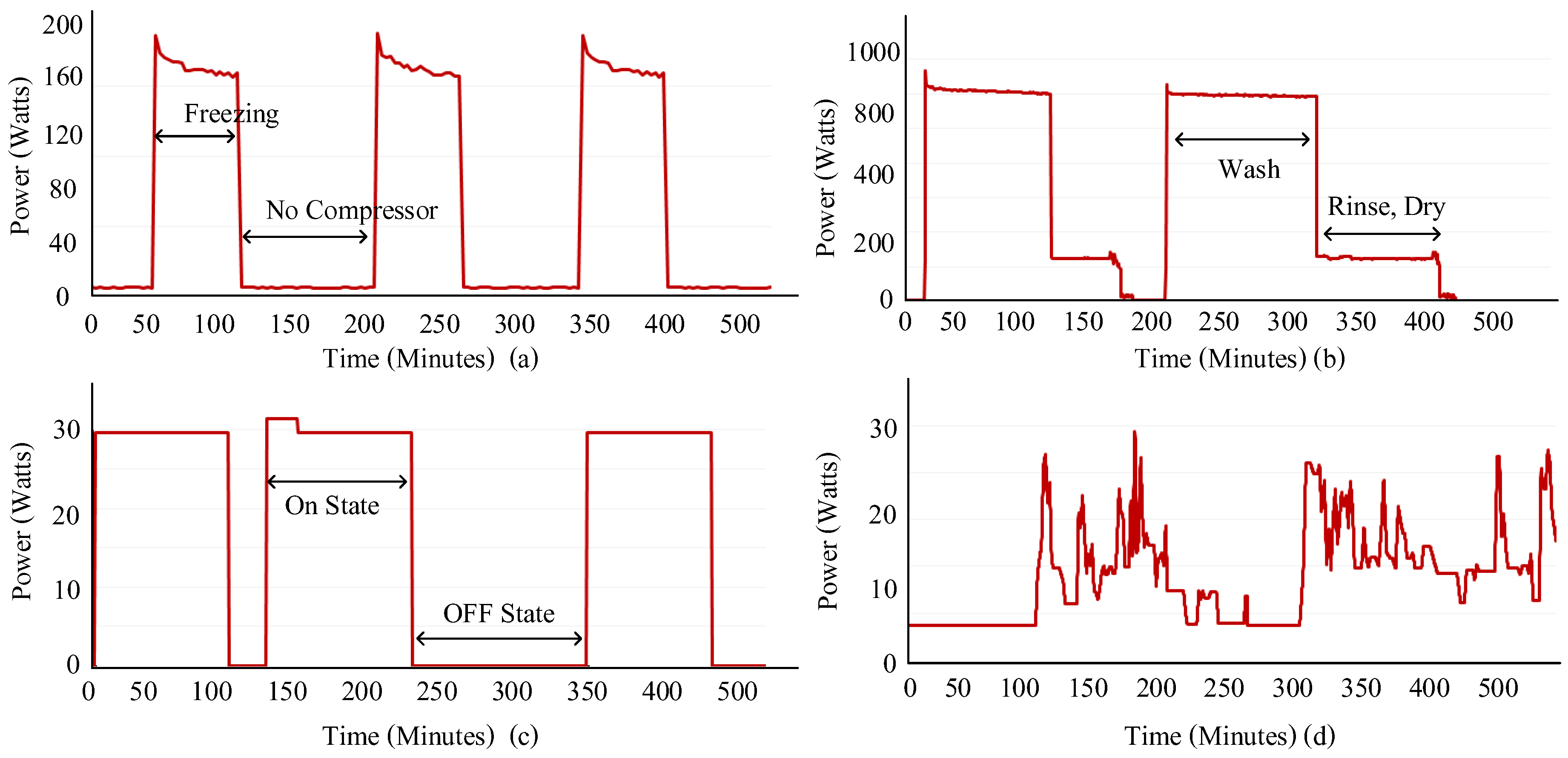
26]. Several appliances are selected from the REDD, DREDD and the AMPds dataset at a sampling rate of 60 s. The appliances are chosen from different appliance categories as discussed in
Section 2.2 to ensure the feasibility of the metric across different appliance categories.
The MEC algorithms are implemented in their sequential order as shown in
Figure 5. In the first step, Algorithm 2, i.e., the appliance state clustering process is implemented on the ground truth data of the fridge. In this process, Algorithm 2 identifies the operational states of the fridge as shown in
Figure 7. This includes the computation of the required parameters and thresholds to improve the performance of event classification and energy estimation as illustrated in Algorithm 2.
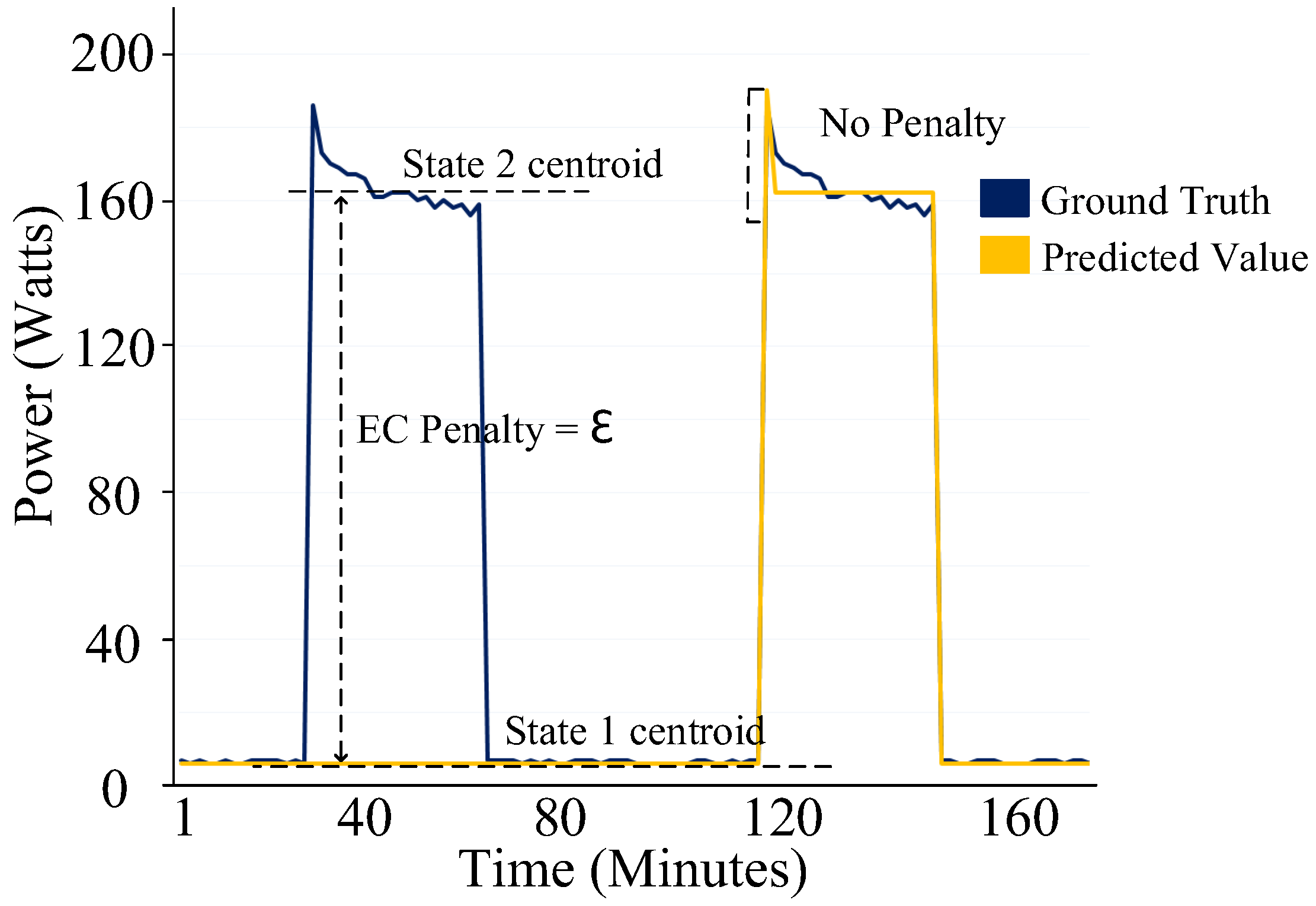
The second step of the implementation is Algorithm 3, i.e., the event classification penalty process.
Figure 8 shows the implementation of this process on the fridge. In this process, each data point
of the ground truth and its corresponding predicted value
is assigned a state of its closest centroid
. A penalty is assigned if the assigned states of the ground truth and its corresponding predicted value do not match. Algorithm 3 outputs
.
The third step of the implementation is Algorithm 4, i.e., the energy estimation penalty process. As shown in
Figure 9, this process divides the ground truth and its corresponding predicted value time series of a fridge into several windows i.e., N, N + 1, N + 2, etc. Algorithm 4 then penalizes incorrect energy estimation. As illustrated in
Figure 9, an incorrect energy estimation is due to the different estimation of states (window N + 1) or to the inaccurate estimation of energy in the same state (window N + 5). The algorithm considers both these scenarios and assigns a penalty accordingly. Algorithm 4 outputs
.
The total penalty as defined in Equation (
4) is applied to precision and recall while the definition of F-score remains the same. Therefore precision and recall for a fridge is now defined as
where
represents on state samples labelled as on state (true positive),
represents off state samples labelled as on state (false positive), and
represents the on state samples labelled as off (false negative). Therefore, the F-score evaluating the performance of NILM algorithm is defined as follows:
Table 1 presents the accuracy scores of two state-of-the art disaggregation algorithms FHMM and SparseViterbi using various metrics. Due to lack of space, we show the results for the user-specified
, i.e., equal weighting to event classification and energy estimation. However, it can be varied (between 0 and 1) according to the user’s emphasis on event classification or energy estimation needs. In the MEC metric, the EC penalty and the EE penalty allows user to directly infer if the NILM algorithm is penalized more for event misclassification or variation in the energy estimation of the state. In type-I (on/off) appliance categories, the MEC metric tends to provide similar accuracies as that of MF-score and FS F-score as shown in
Table 1. This is because type-I (on/off) devices do not have multiple active states to classify and therefore will not be penalized for incorrect classification of the operational states by MEC. However, the MEC metric results show a noticeable decrease in accuracy for multiple state appliance categories such as type-II (finite state machines or multi-state appliances) and type-IV (always on) for various datasets. This is due to the incorrect classification of multiple operational states and inaccurate energy estimation by other metrics as shown in
Table 1.
5. Conclusions and Future Works
This paper proposed a new MEC metric that addressed the three issues with existing state-of-the-art metrics: a lack of a unified metric that reflects both state classification and energy estimation at the same time; accurate penalization of predictions that are too far from the ground truth in the context of a state; and the accurate classification of multi-state appliances. The proposed metric solves these issues by combining energy estimation with event classification to accurately quantify and penalize the algorithm. In this work, we used unsupervised clustering techniques to identify the operational states of the device from a labelled dataset to compute a penalty threshold for predictions that are too far away from the ground truth.
In our experimental results, the MEC exhibits the intuitive nature of the metric using state-of-the-art disaggregation algorithms. Existing metrics such as M F-score and FS F-score have reported higher accuracies due to inaccurate state classification and incorrect penalization of energy estimation respectively. However, our MEC metric provides better results over several datasets and devices from different appliance categories. The MEC accurately quantifies and penalizes the state misclassification and variation in the energy estimation of a state.
From the implemented MEC metric results, the MEC performs well in accurately evaluating the performance of various disaggregation algorithms with respect to event classification and energy estimation. Therefore, we are planning to use MEC metric accuracy as a means to quantify the noise needed to obfuscate a power consumption time series for privacy preservation as our future work.
