In-Depth Analysis of Unmodulated Visible Light Positioning Using the Iterated Extended Kalman Filter


Abstract
:1. Introduction
2. Related Work
- We provide much more in-depth simulations, to better characterize the limits of this approach. Among other factors, we investigate the influence of:
- -
- Partial shadowing
- -
- Random trajectories
- -
- Robot movement speed
- -
- Imperfect calibration
- We validated the approach with experimental data.
3. Materials and Methods
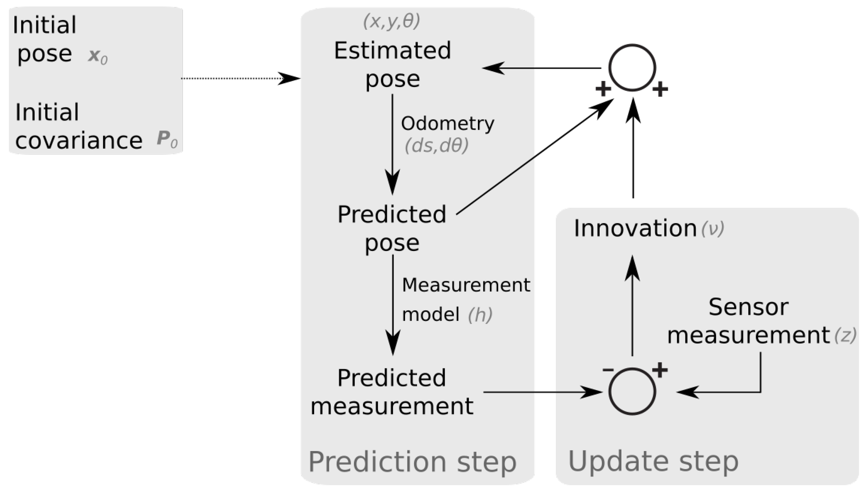
3.1. IEKF Formulation
3.2. Simulation Environment
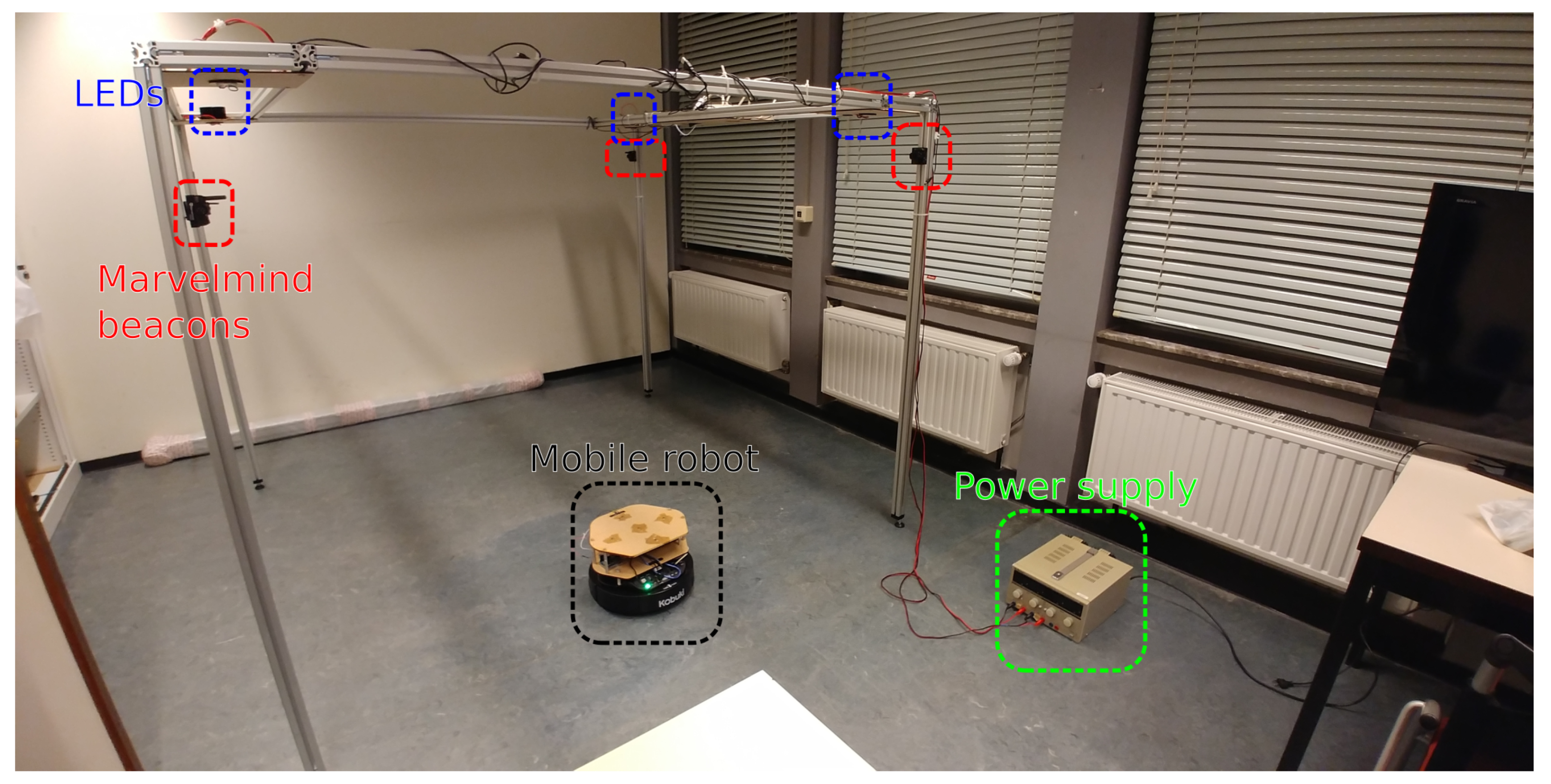
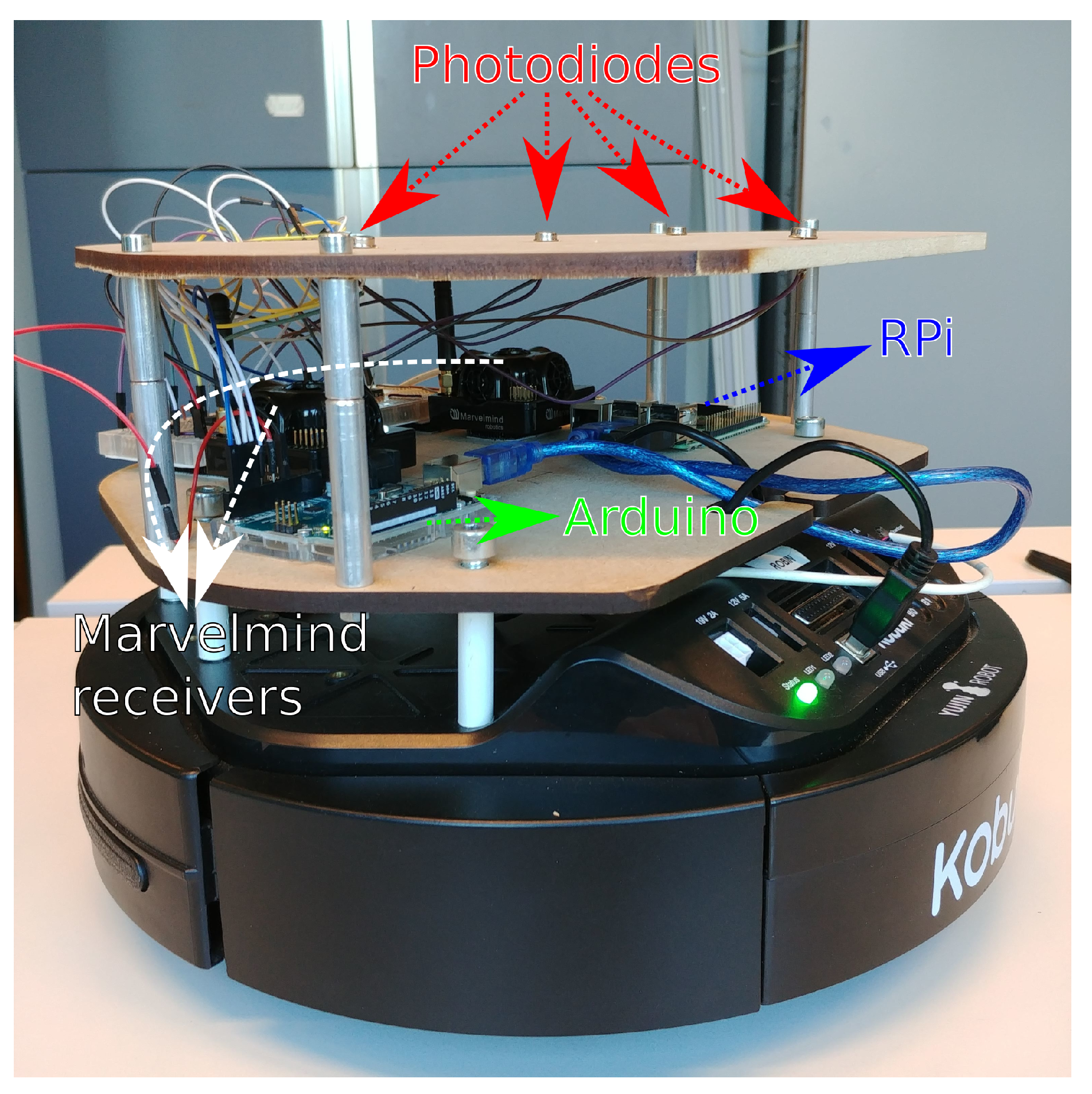
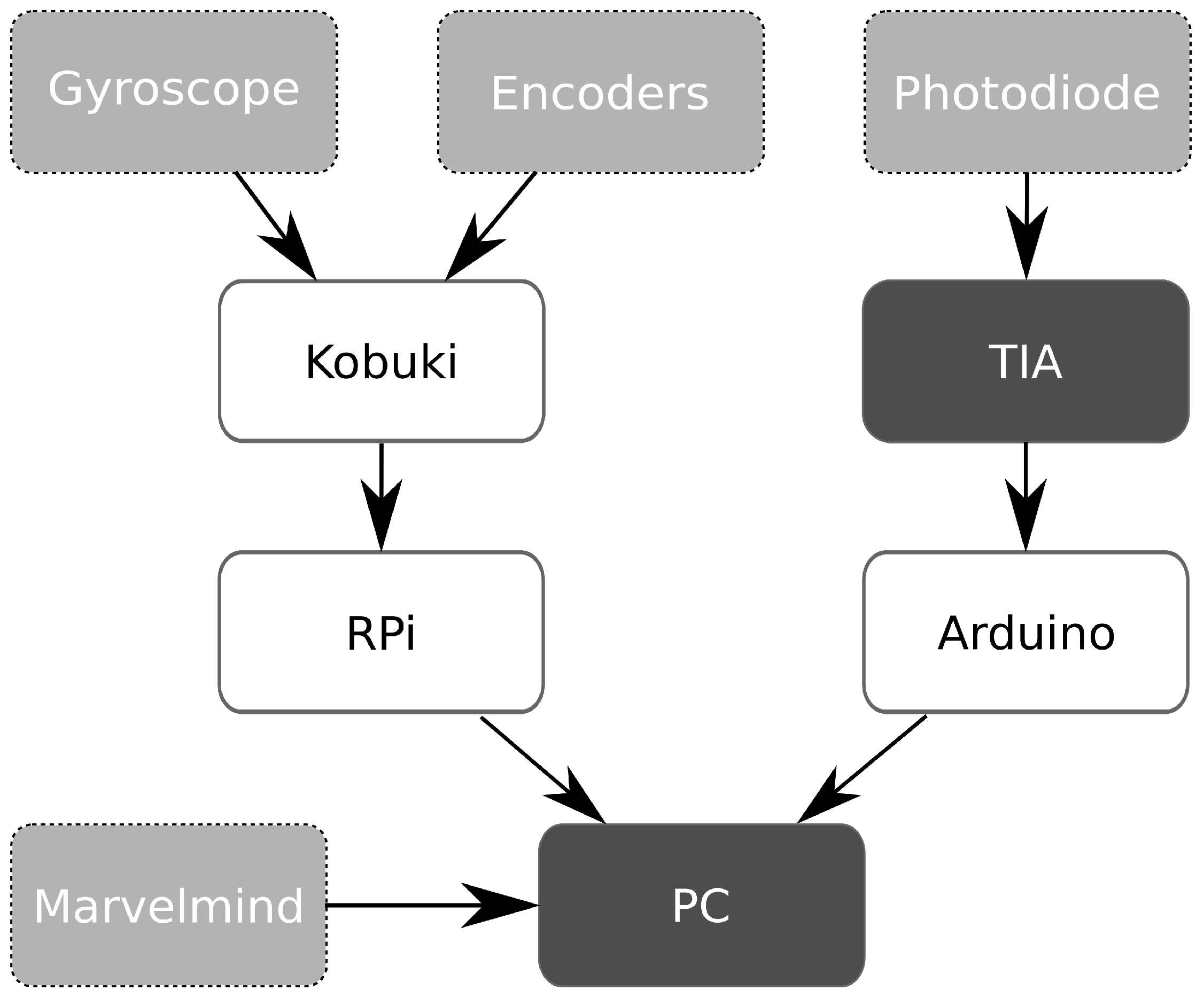
3.3. Experimental Setup
4. Simulation Results
4.1. Single Receiver Results
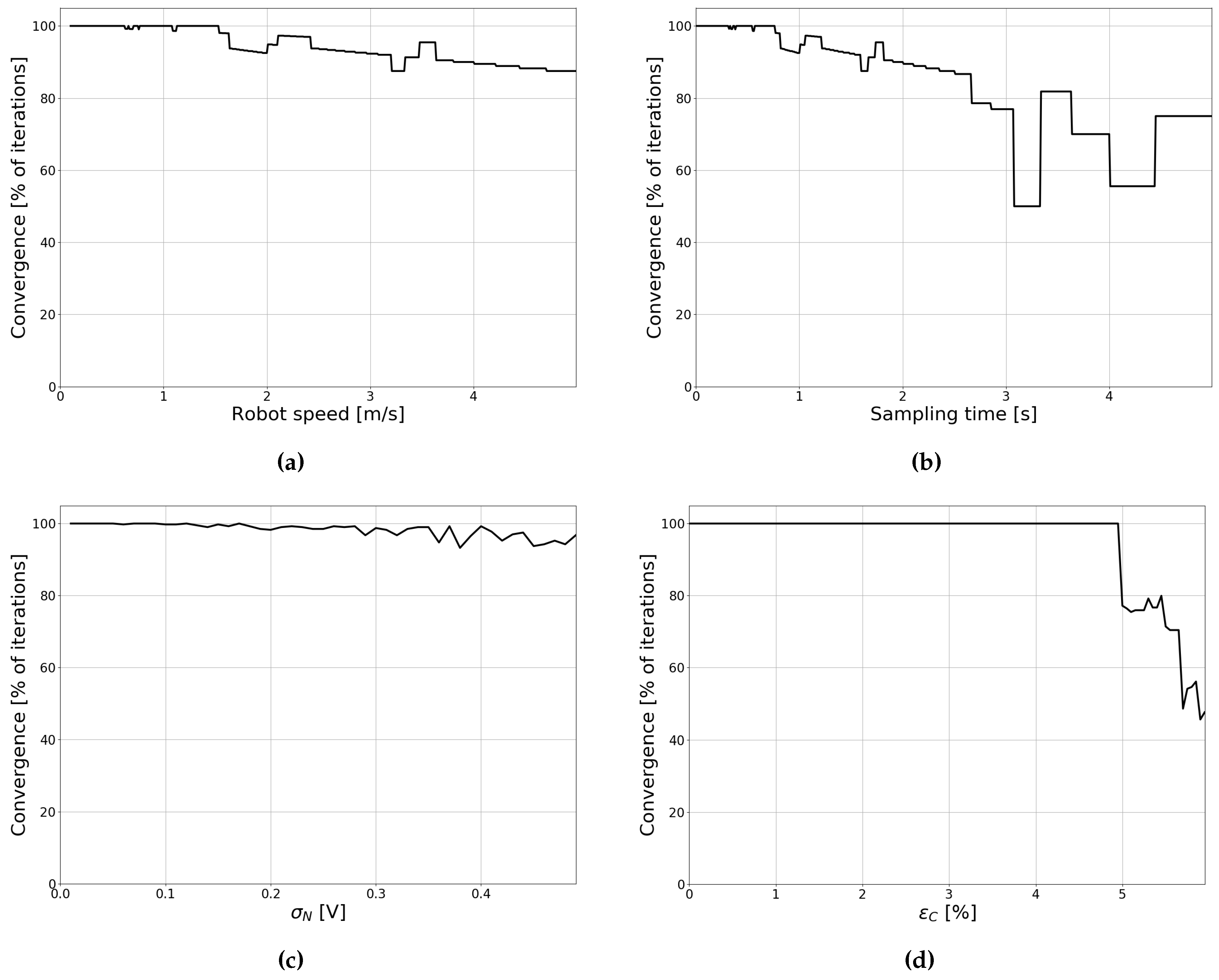
4.1.1. Convergence
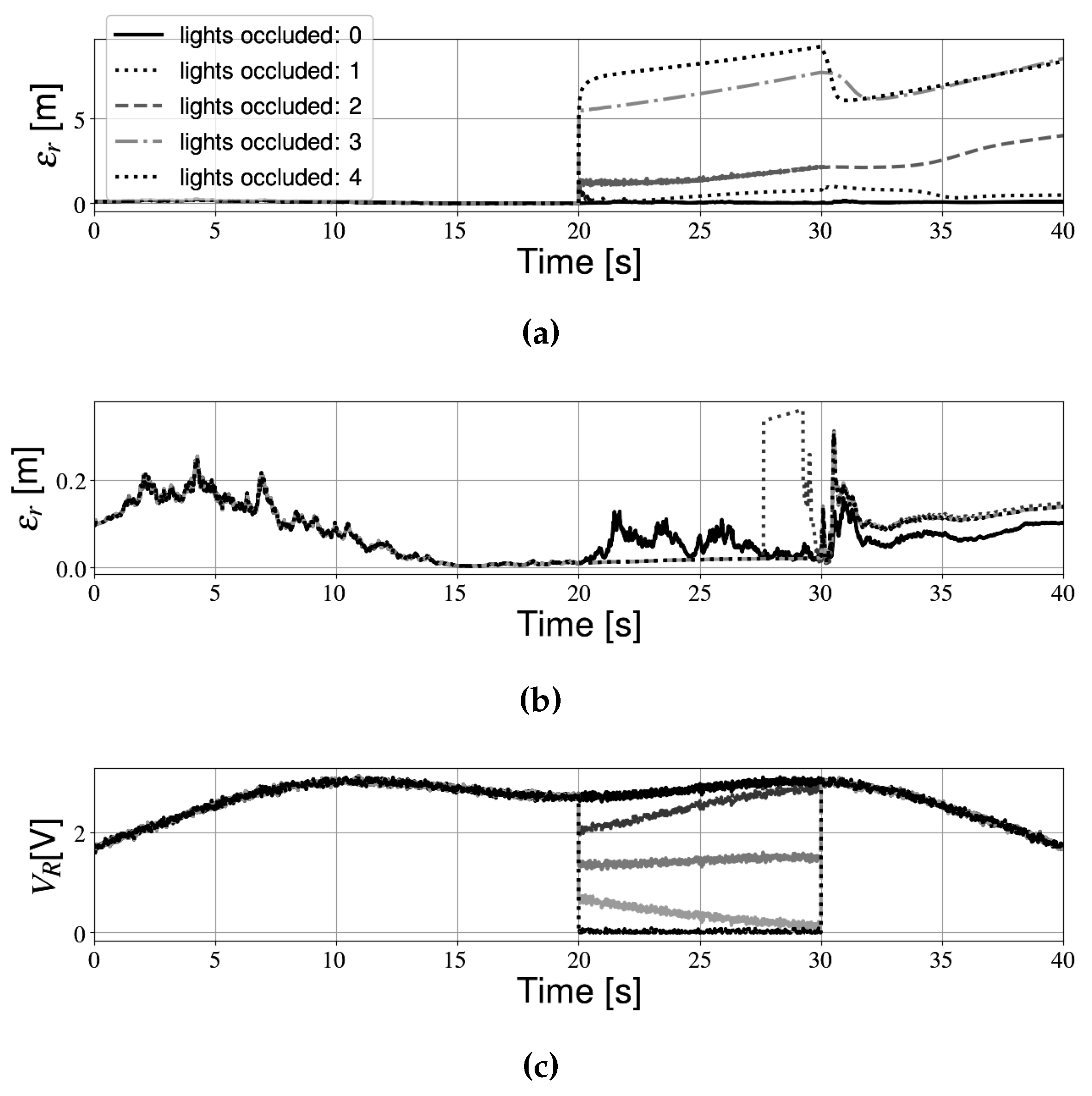
4.1.2. Shadowing of the Receiver
4.1.3. Innovation Magnitude Bounds Test
4.2. Multiple Receiver Results
4.2.1. Shadowing of Multiple Receivers
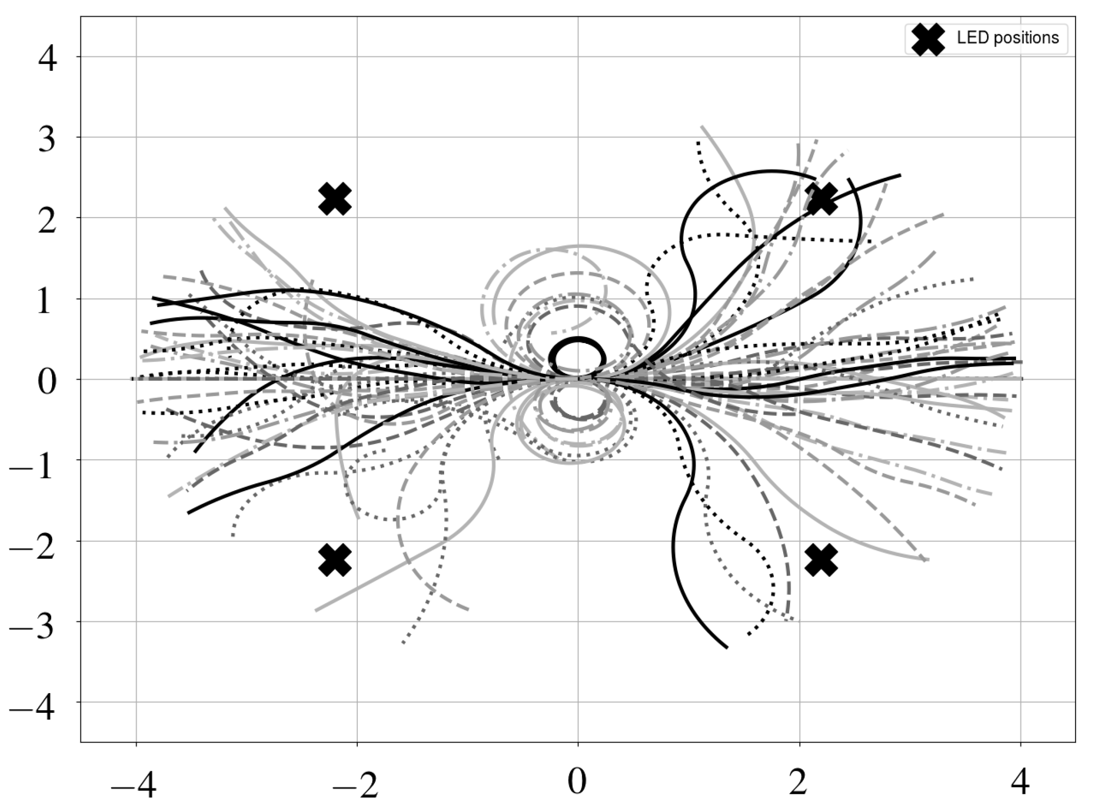
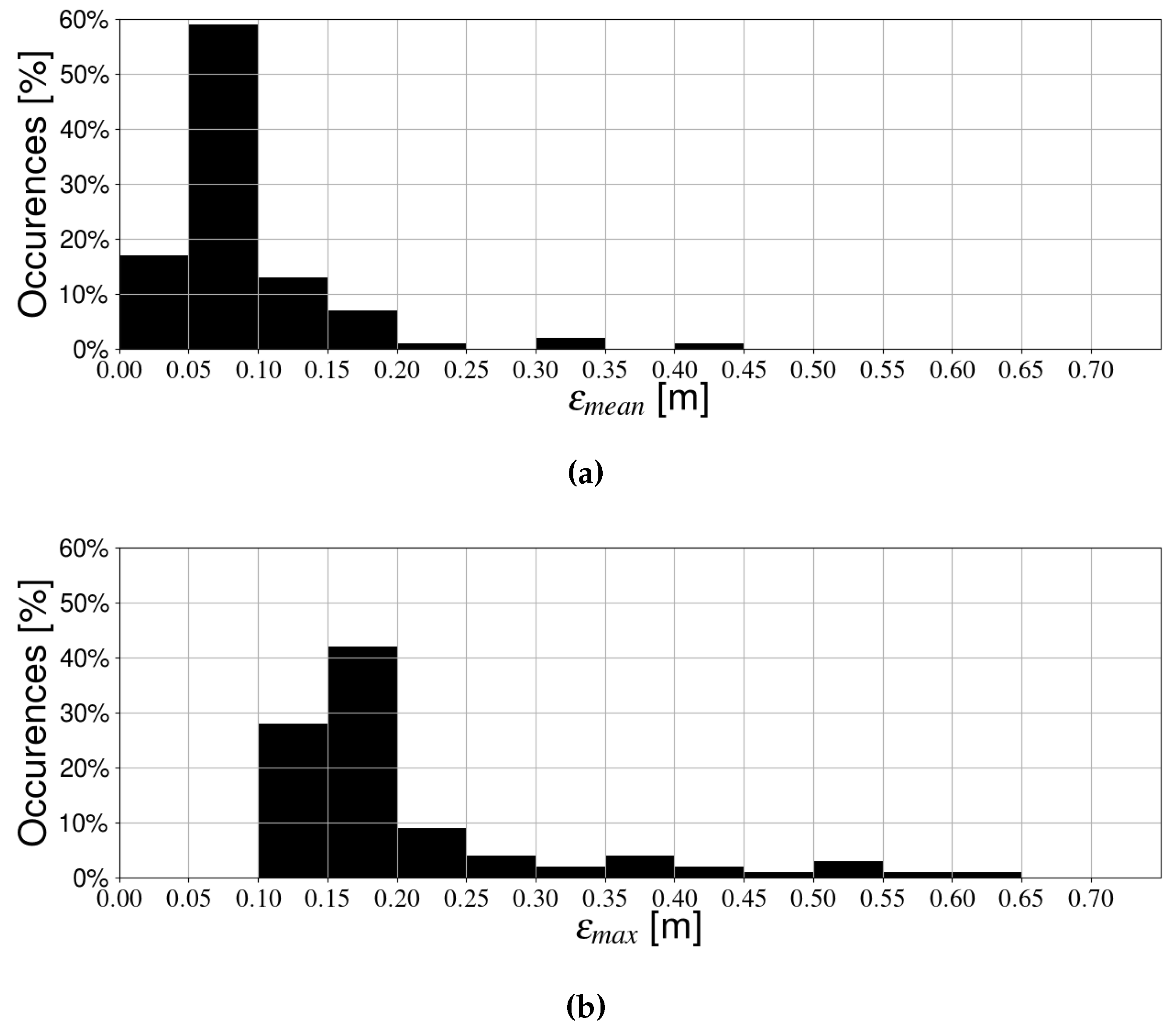
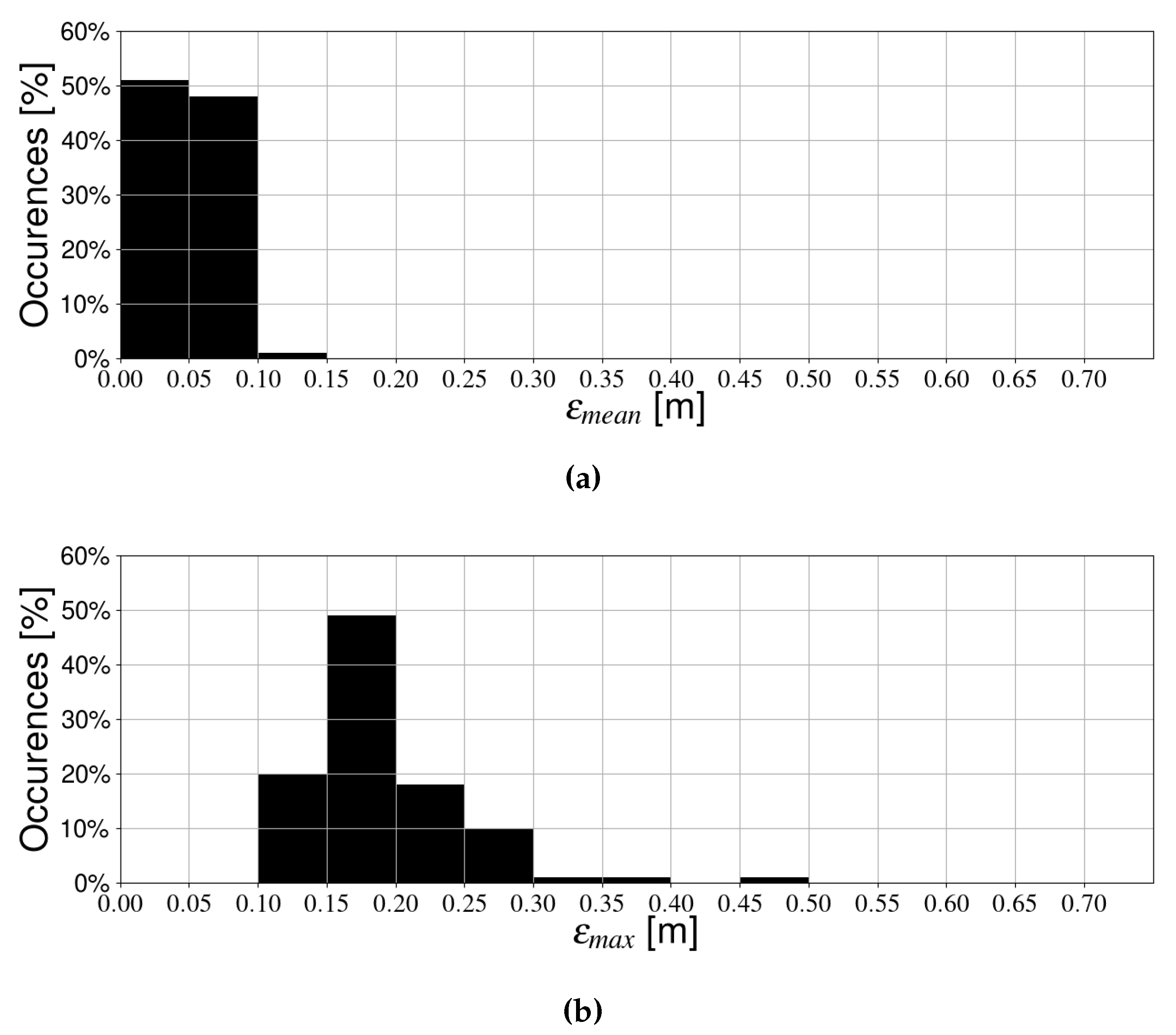
4.3. Random Trajectories
- Obtain the total number of iterations as: , where L is the length of the trajectory, v is the forward speed of the robot, and T is the sampling time.
- Obtain the initial pose. For all trajectories, the initial position coincides with the origin. Half of the poses were initialized with a heading angle of 0 degrees, the other half have an orientation of 180 degrees.
- Select the number of turns () in the trajectory as a random number between 0 and 10.
- Calculate the angle that will be covered in each turn (), which is a random number between −30 and 30 degrees.
- Determine the angular displacement between estimates (), such that the angle is covered in iterations.
- Determine the displacement between estimates as a random number between 0 and .
4.4. Parameter Errors
5. Experimental Results
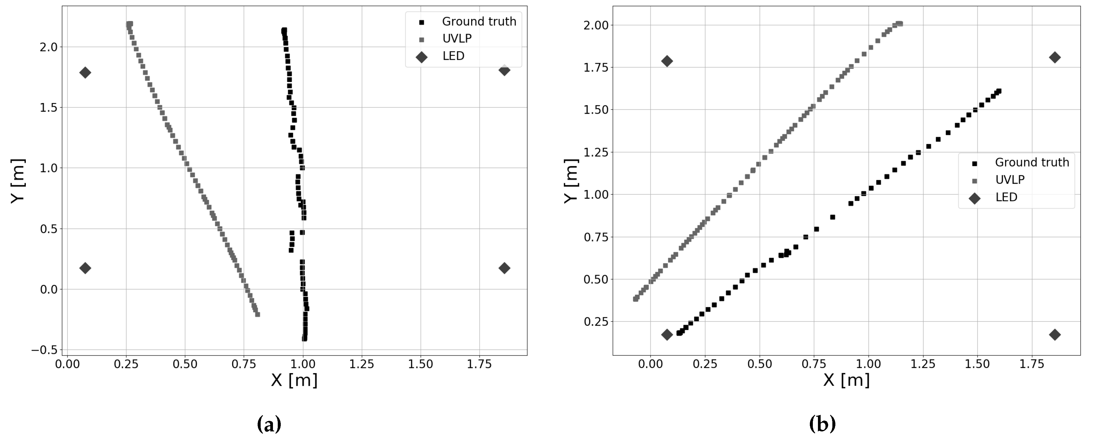
5.1. Overview
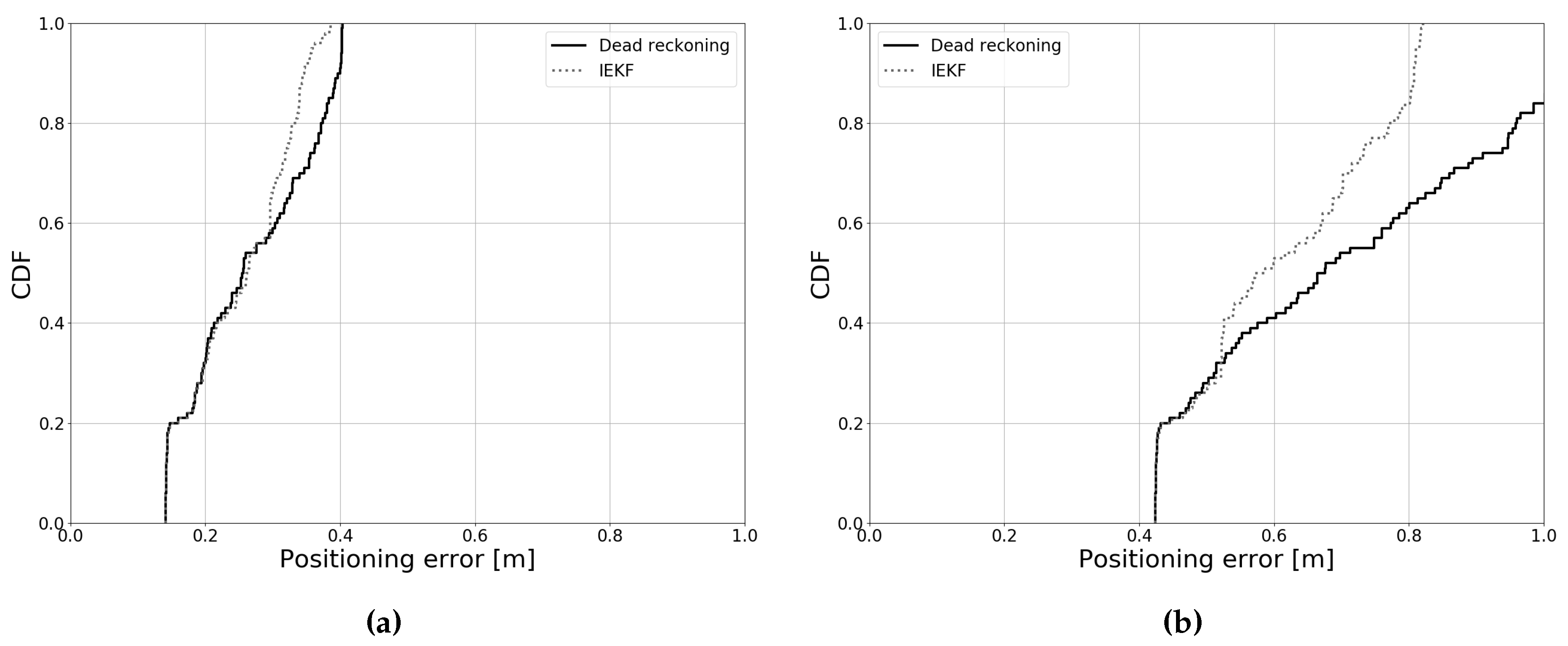
- Dead reckoning: Only odometry measurements were used for position estimation. These results mainly provide a comparison for the estimates that include light measurements. Overall filter performance depended on the accuracy of dead reckoning. Hence, mainly the improvement over this case was of interest.
- 1 receiver: Light intensity measurements from a single photodiode were used. This represents the simplest possible case for our proposed approach.
- 5 receivers: Light intensity measurements from five photodiodes were used for position estimation.
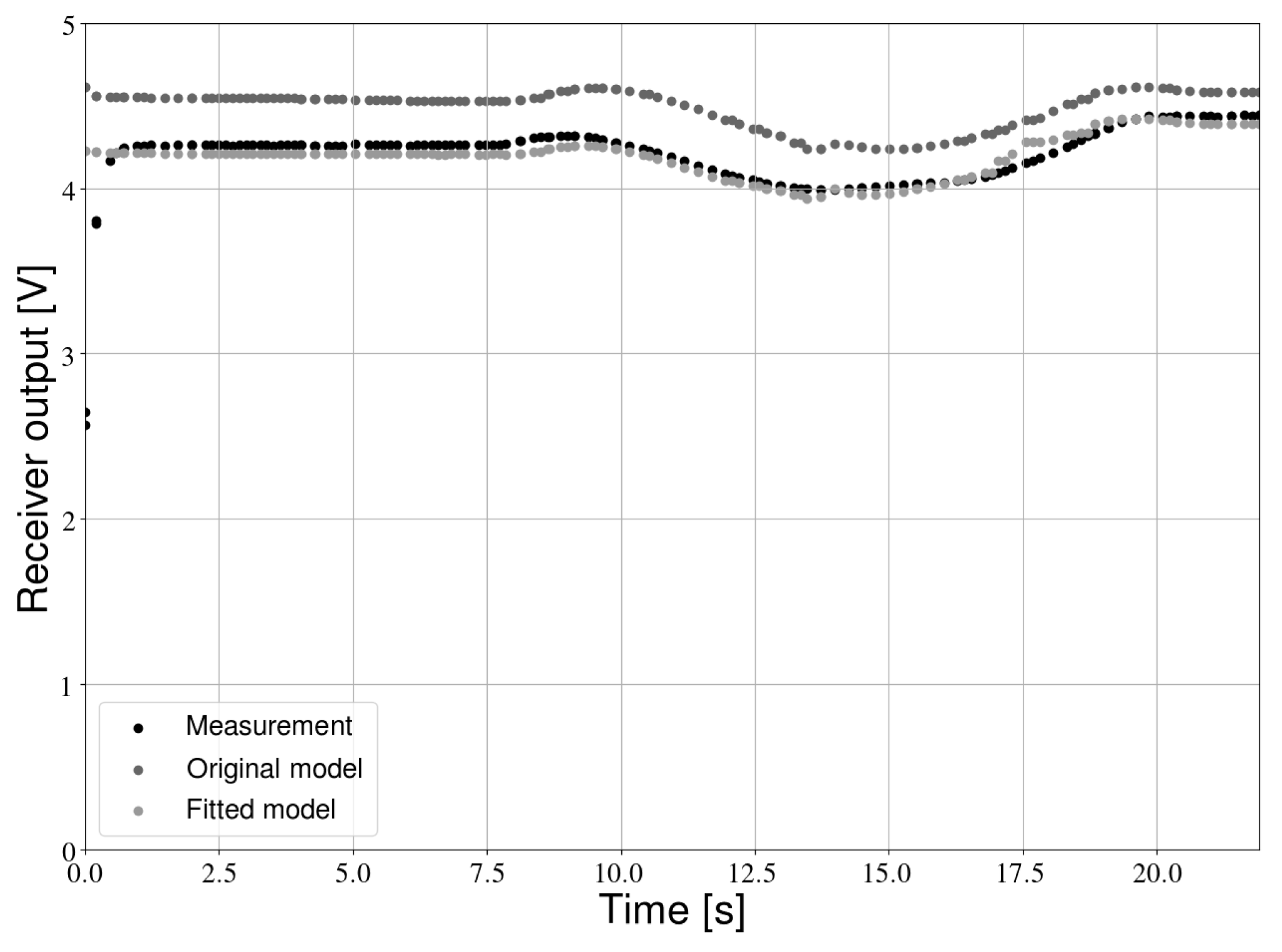
5.2. Verification of the Measurement Model
5.3. Initial Position Estimate
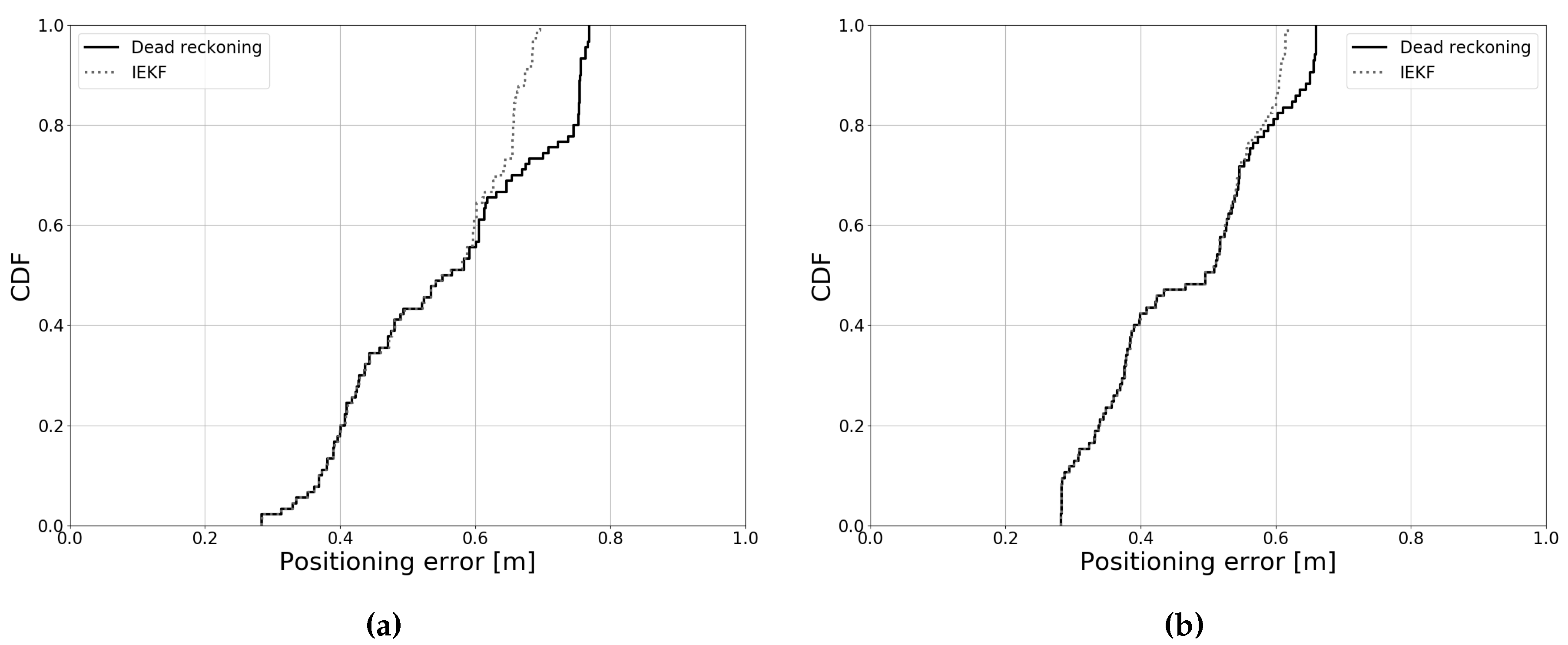
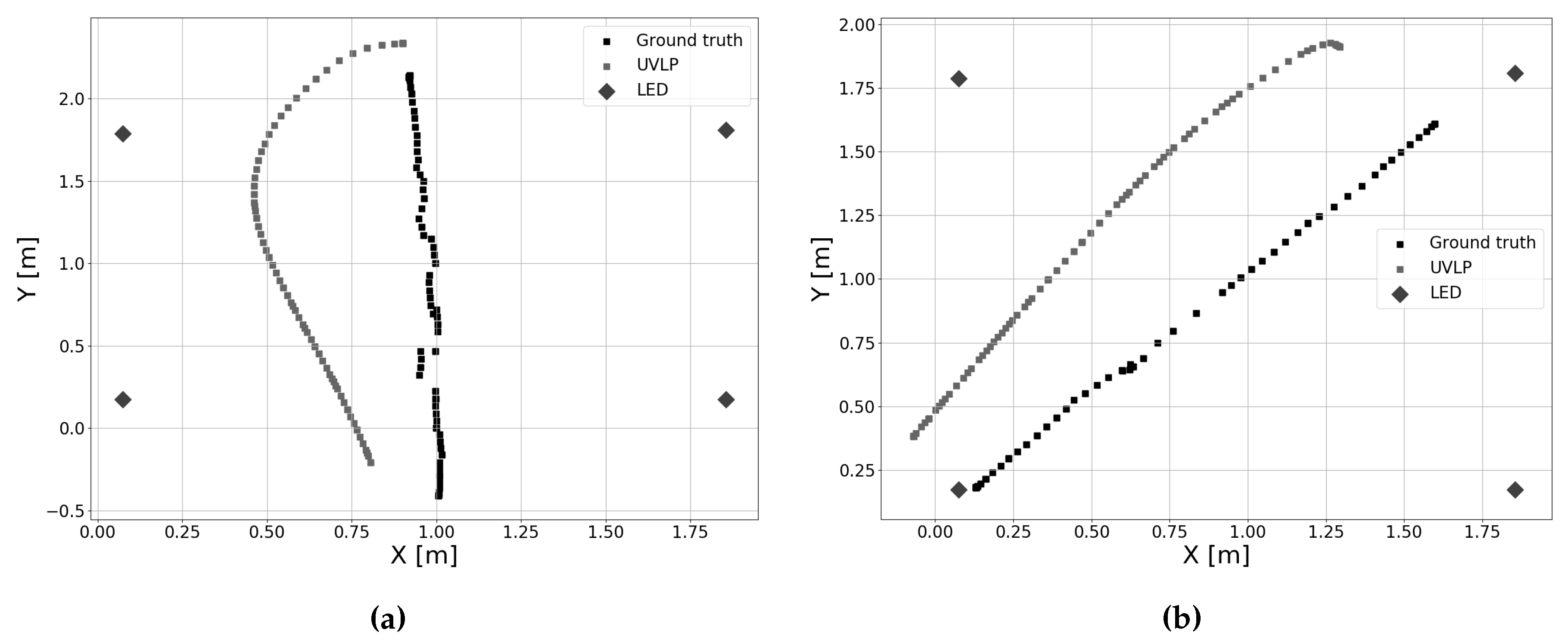
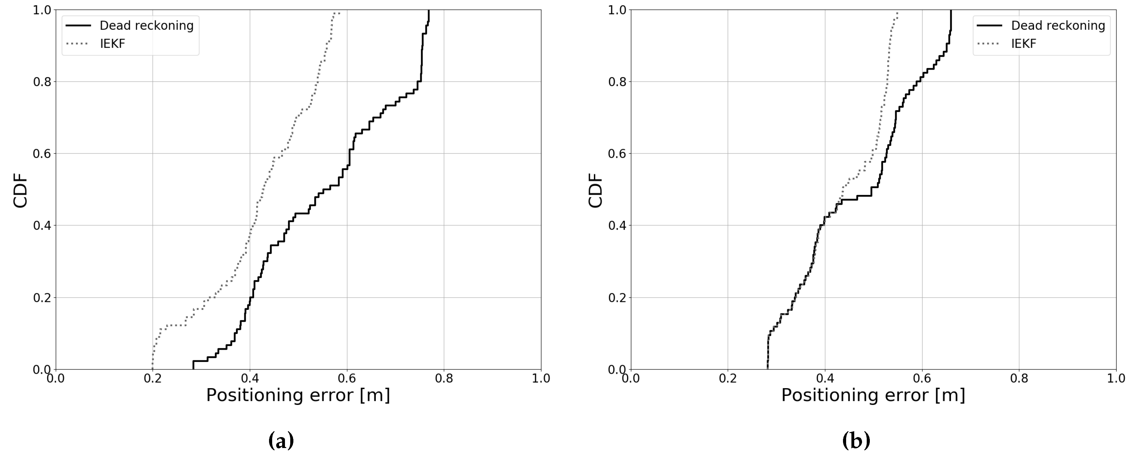
5.4. Single Receiver Results
5.5. Multiple Receiver Results
6. Discussion
7. Conclusions
Author Contributions
Funding
Conflicts of Interest
References
- Mautz, R. Indoor Positioning Technologies. Ph.D. Thesis, ETH Zurich, Zürich, Switzerland, 2012. [Google Scholar]
- Bejuri, W.M.; Wan, Y.; Mohamad, M.; Sapri, M. Ubiquitous Positioning: A Taxonomy for Location Determination on Mobile Navigation System. arXiv 2011, arXiv:1103.5035. [Google Scholar]
- Gu, Y.; Lo, A.; Niemegeers, I. A Survey of Indoor Positioning Systems for Wireless Personal Networks. IEEE Commun. Surv. Tutor. 2009, 11, 13–32. [Google Scholar] [CrossRef]
- Dabove, P.; Di Pietra, V.; Piras, M.; Jabbar, A.A.; Kazim, S.A. Indoor Positioning Using Ultra-wide Band (UWB) Technologies: Positioning Accuracies and Sensors’ Performances. In Proceedings of the 2018 IEEE/ION Position, Location and Navigation Symposium, Monterey, CA, USA, 23–26 April 2018; pp. 175–184. [Google Scholar]
- Statler, S. Beacon Technologies; Springer: Berlin/Heidelberg, Germany, 2016. [Google Scholar]
- Makki, A.; Siddig, A.; Saad, M.; Bleakley, C. Survey of WiFi Positioning Using Time-based Techniques. Comput. Netw. 2015, 88, 218–233. [Google Scholar] [CrossRef]
- Zhuang, Y.; Hua, L.; Qi, L.; Yang, J.; Cao, P.; Cao, Y.; Wu, Y.; Thompson, J.; Haas, H. A Survey of Positioning Systems Using Visible LED Lights. IEEE Commu. Surv. Tutor. 2018, 20, 1963–1988. [Google Scholar] [CrossRef]
- Global LED Lighting Market: Forecast by Applications, Regions and Companies. Technical Report, Renub Research. 2017. Available online: https://www.researchandmarkets.com/reports/4437008/global-led-lighting-market-forecast-by (accessed on 12 April 2019).
- Haas, H.; Yin, L.; Wang, Y.; Chen, C. What is LiFi? J. Lightware Technol. 2015, 34, 1533–1544. [Google Scholar] [CrossRef]
- Ghassemlooy, Z.; Popoola, W.; Rajbhandari, S. Optical Wireless Communications: System and Channel Modelling with Matlab®; CRC Press: Boca Raton, FL, USA, 2012. [Google Scholar]
- Do, T.H.; Yoo, M. An in-Depth Survey of Visible Light Communication Based Positioning Systems. Sensors 2016, 16, 678. [Google Scholar] [CrossRef] [PubMed]
- Yang, H.; Du, P.; Zhong, W.; Chen, C.; Alphones, A.; Zhang, S. Reinforcement Learning-Based Intelligent Resource Allocation for Integrated VLCP Systems. IEEE Wirel. Commun. Lett. 2019, 8, 1204–1207. [Google Scholar] [CrossRef]
- Du, P.; Zhang, S.; Chen, C.; Alphones, A.; Zhong, W.D. Demonstration of a Low-Complexity Indoor Visible Light Positioning System Using an Enhanced TDOA Scheme. IEEE Photonics J. 2018, 10, 1–10. [Google Scholar] [CrossRef]
- Claudio, F.; Tièche, F.; Hügli, H. Self-Positioning Robot Navigation Using Ceiling Image Sequences. In Proceedings of the Asian Conference on Computer Vision, Singapore, 5–8 December 1995; pp. 814–818. [Google Scholar]
- Panzieri, S.; Pascucci, F.; Setola, R.; Ulivi, G. A Low Cost Vision Based Localization System for Mobile Robots. Target 2001, 4, 1–6. [Google Scholar]
- Wang, H.; Ishimatsu, T.; Mian, J.T. Self-Localization for an Electric Wheelchair. JSME Int. J. Ser. C 1997, 40, 433–438. [Google Scholar] [CrossRef]
- Launay, F.; Ohya, A.; Yuta, S. A Corridors Lights based Navigation System including Path Definition using a Topologically Corrected Map for Indoor Mobile Robots. In Proceedings of the 2002 IEEE International Conference on Robotics and Automation, Washington, DC, USA, 11–15 May 2002; pp. 3918–3923. [Google Scholar]
- Chen, X.; Jia, Y. Indoor Localization for Mobile Robots Using Lampshade Corners as Landmarks: Visual System Calibration, Feature Extraction and Experiments. Int. J. Control Autom. Syst. 2014, 12, 1313–1322. [Google Scholar] [CrossRef]
- Lausnay, S.D.; Strycker, L.D.; Goemaere, J.P.; Nauwelaers, B.; Stevens, N. A survey on multiple access Visible Light Positioning. In Proceedings of the 2016 IEEE International Conference on Emerging Technologies and Innovative Business Practices for the Transformation of Societies (EmergiTech), Balaclava, Mauritius, 3–6 August 2016; pp. 38–42. [Google Scholar]
- Ravi, N.; Iftode, L. FiatLux: Fingerprinting Rooms Using Light Intensity; NA Publishing: Ann Arbor, MI, USA, 2007. [Google Scholar]
- Golding, A.; Lesh, N. Indoor Navigation Using a Diverse Set of Cheap, Wearable Sensors. In Proceedings of the Third International Symposium on Wearable Computers, San Francisco, CA, USA, 18–19 October 1999; pp. 29–36. [Google Scholar]
- Azizyan, M.; Constandache, I.; Roy Choudhury, R. SurroundSense: Mobile Phone Localization via Ambience Fingerprinting. In Proceedings of the 15th annual international conference on Mobile computing and networking, Beijing, China, 20–25 September 2009; pp. 261–272. [Google Scholar]
- Zhang, C.; Zhang, X. LiTell: robust indoor localization using unmodified light fixtures. In Proceedings of the 22nd Annual International Conference on Mobile Computing and Networking, New York, NY, USA, 3–7 October 2016; pp. 230–242. [Google Scholar]
- Wang, Q.; Wang, X.; Ye, L.; Men, A.; Zhao, F.; Luo, H.; Huang, Y. A Multimode Fusion Visible Light Localization Algorithm Using Ambient Lights. In Proceedings of the 5th IEEE Conference on Ubiquitous Positioning, Indoor Navigation and Location-Based Services, Wuhan, China, 22–23 March 2018; pp. 1–9. [Google Scholar]
- Jiménez, A.; Zampella, F.; Seco, F. Improving Inertial Pedestrian Dead-Reckoning by Detecting Unmodified Switched-on Lamps in Buildings. Sensors 2014, 14, 731–769. [Google Scholar] [CrossRef] [PubMed]
- Hu, Y.; Xiong, Y.; Huang, W.; Li, X.Y.; Zhang, Y.; Mao, X.; Yang, P.; Wang, C. Lightitude: Indoor Positioning Using Ubiquitous Visible Lights and COTS Devices. In Proceedings of the International Conference on Distributed Computing Systems, Columbus, OH, USA, 29 June–2 July 2015; pp. 732–733. [Google Scholar]
- Xu, Q.; Zheng, R.; Hranilovic, S. IDyLL: Indoor Localization using Inertial and Light Sensors on Smartphones. In Proceedings of the 2015 ACM International Joint Conference on Pervasive and Ubiquitous Computing, Osaka, Japan, 7–11 September 2015; pp. 307–318. [Google Scholar]
- Amsters, R.; Demeester, E.; Stevens, N.; Slaets, P. Unmodulated Visible Light Positioning using the Iterated Extended Kalman Filter. In Proceedings of the 2018 International Conference on Indoor Positioning and Indoor Navigation (IPIN), Nantes, France, 24–27 September 2018; pp. 1–8. [Google Scholar]
- Havlík, J.; Straka, O. Performance evaluation of iterated extended Kalman filter with variable step-length. In Proceedings of the 12th European Workshop on Advanced Control and Diagnosis, Pilsen, Czech Republic, 19–20 November 2015; p. 012022. [Google Scholar]
- Thrun, S.; Burgard, W.; Fox, D. Probabilistic Robotics; MIT Press: Cambridge, MA, USA, 2005. [Google Scholar]
- Kahn, J.M.; Barry, J.R. Wireless infrared communications. Proc. IEEE 1997, 85, 265–298. [Google Scholar] [CrossRef]
- Yujin Robot. KOBUKI|Kobuki|Waiterbot|Shooter. Available online: http://kobuki.yujinrobot.com/ (accessed on 7 August 2019).
- Amsters, R.; Demeester, E.; Stevens, N.; Lauwers, Q.; Slaets, P. Evaluation of Low-Cost/High-Accuracy Indoor Positioning Systems. In Proceedings of the 2019 International Conference on Advances in Sensors, Actuators, Metering and Sensing (ALLSENSORS), Athens, Greece, 24–28 February 2019; pp. 15–20. [Google Scholar]
- Bar-Shalom, Y.; Li, X.R.; Kirubarajan, T. Estimation with Applications to Tracking and Navigation: Theory Algorithms and Software; John Wiley & Sons: Hoboken, NJ, UAS, 2004. [Google Scholar]
- Jiménez, A.R.; Zampella, F.; Seco, F. Light-matching: A new signal of opportunity for pedestrian indoor navigation. In Proceedings of the 2013 International Conference on Indoor Positioning and Indoor Navigation, Montbeliard-Belfort, France, 28–31 October 2013; pp. 1–10. [Google Scholar]
- Gutmann, J.S.; Burgard, W.; Fox, D.; Konolige, K. An experimental comparison of localization methods. In Proceedings of the 1998 IEEE/RSJ International Conference on Intelligent Robots and Systems Innovations in Theory, Practice and Applications (Cat. No. 98CH36190), Victoria, BC, Canada, 17 October 1998; pp. 736–743. [Google Scholar]
- Conti, G.; Malabocchia, F.; Li, K.J.; Percivall, G.; Burroughs, K.; Strickland, S. Benefits of Indoor Location, Use Case Survey of Lessons Learned and Expectations. Technical Report. 2016. Available online: https://portal.opengeospatial.org/files/?artifact_id=68604&usg=AOvVaw16eOF9lRQsNqp55F5Ia-M- (accessed on 29 November 2019).


| Component | Manufacturer | Model Name |
|---|---|---|
| LED | Bridgelux | BXRC-50E4000-F-24 |
| Photodiode | Osram | BPX 61 |
| Robot platform | Yujin Robot | Kobuki |
| Microcontroller | CC Logistics LLC | Arduino UNO |
| Embedded board | Raspberry Pi 3 | Raspberry Pi Foundation |
| Ground truth location reference | Starter set (433 MHz) | Marvelmind Robotics |
| Symbol | Description | Value | Unit |
|---|---|---|---|
| Receiver parameters | |||
| A | Area of receiver | 7.02 | mm2 |
| G | TIA Gain | 500 | kOhm |
| Peak responsivity of photodiode | 0.62 | A/W | |
| FET transinductance | 30 | mS | |
| FET noise factor | 1.5 | / | |
| Capacitance per unit area | 1.026 × 10⁻¹¹ | F/mm2 | |
| Noise bandwidth parameter | 0.562 | / | |
| Noise bandwidth parameter | 0.0868 | / | |
| Background current | 190 | A | |
| Equivalent noise bandwidth | 100 | MHz | |
| Transmitter parameters | |||
| Luminous flux | 4275 | lm | |
| m | Order of Lambertian emission | 1 | / |
| Half power angle | 60 | ||
| CCT | Correlated color temperature | 5000 | K |
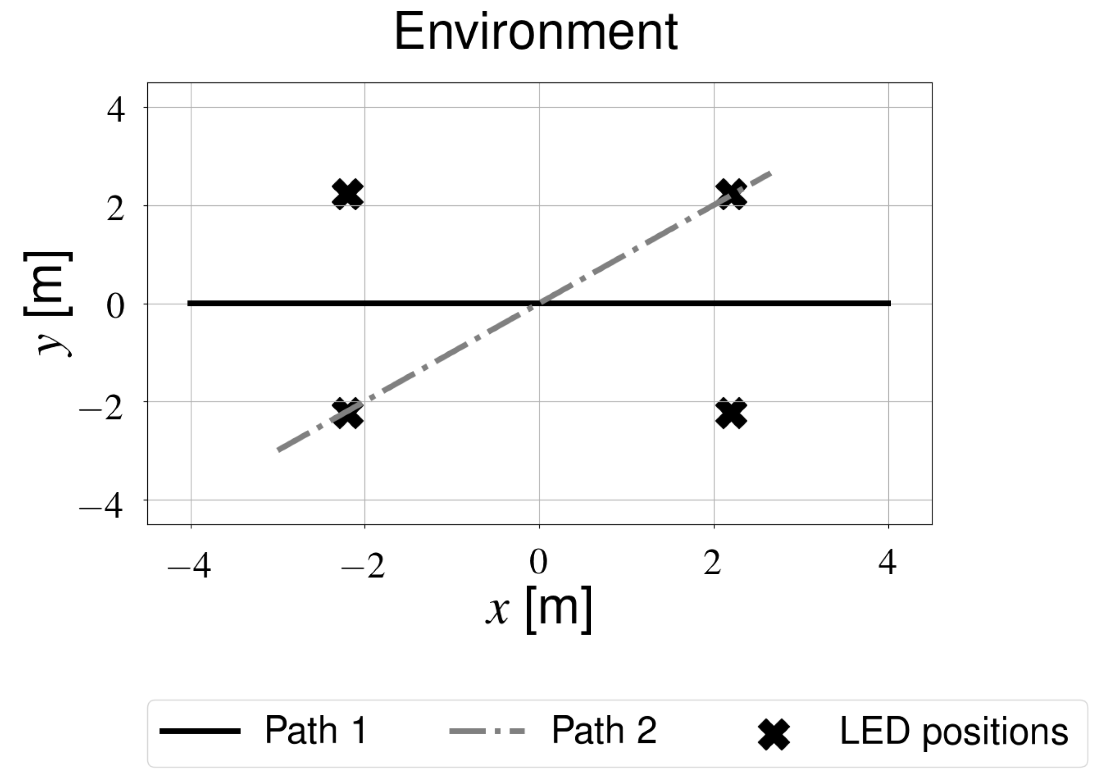
| Position LED [x,y] | [−2.20, −2.235] | m | |
| Position LED [x,y] | [2.20, −2.235] | m | |
| Position LED [x,y] | [2.20, 2.235] | m | |
| Position LED [x,y] | [−2.20, 2.235] | m | |
| Simulation parameters | |||
| Duration of time step | 0.1 | s | |
| Height difference of receiver and transmitter | 2.8 | m | |
| T | Ambient temperature | 293 | K |
| Filter parameters | |||
| Maximum number of update iterations | 10 | / | |
| Minimum distance between subsequent IEKF iterations | 0.05 | m | |
| Initial variance on x-coordinate | 0.04 | m2 | |
| Initial variance on y-coordinate | 0.04 | m2 | |
| Initial variance on heading angle | 0.05 | radians2 | |
| Variance on odometry distance measurements | 3.60 × 10⁻⁹ | m2 | |
| Variance on odometry angle measurements | 2.50 × 10⁷ | radians2 | |
| Trajectory | Default | Innovation Bounds |
|---|---|---|
| Path 1 | 2,3,4 | / |
| Path 2 | 2,3,4 | 1 |
| Parameter | Error | Unit |
|---|---|---|
| Ceiling height | 0.01 | m |
| Receiver angle | 1 | |
| Model constant (C in Equation (5)) | 1.5 | % |
| Trajectory | Default | Innovation Bounds |
|---|---|---|
| Path 1 | / | / |
| Path 2 | Single | Single |
| Dataset | Mean Error [m] | P95 Error [m] | Processing Delay [ms] | Maximum Update Rate [Hz] |
|---|---|---|---|---|
| DR, Path 1 | 0.438 | 0.569 | 0.2 | 50 |
| One receiver, Path 1 | 0.406 | 0.502 | 1.2 | 112 |
| Five receivers, Path 1 | 0.336 | 0.464 | 4.3 | 84 |
| DR, Path 2 | 0.321 | 0.408 | 0.2 | 50 |
| One receiver, Path 2 | 0.316 | 0.390 | 1.2 | 112 |
| Five receivers, Path 2 | 0.298 | 0.363 | 4.2 | 84 |
© 2019 by the authors. Licensee MDPI, Basel, Switzerland. This article is an open access article distributed under the terms and conditions of the Creative Commons Attribution (CC BY) license (http://creativecommons.org/licenses/by/4.0/).
Share and Cite
Amsters, R.; Demeester, E.; Stevens, N.; Slaets, P. In-Depth Analysis of Unmodulated Visible Light Positioning Using the Iterated Extended Kalman Filter. Sensors 2019, 19, 5198. https://doi.org/10.3390/s19235198
Amsters R, Demeester E, Stevens N, Slaets P. In-Depth Analysis of Unmodulated Visible Light Positioning Using the Iterated Extended Kalman Filter. Sensors. 2019; 19(23):5198. https://doi.org/10.3390/s19235198
Chicago/Turabian StyleAmsters, Robin, Eric Demeester, Nobby Stevens, and Peter Slaets. 2019. "In-Depth Analysis of Unmodulated Visible Light Positioning Using the Iterated Extended Kalman Filter" Sensors 19, no. 23: 5198. https://doi.org/10.3390/s19235198
APA StyleAmsters, R., Demeester, E., Stevens, N., & Slaets, P. (2019). In-Depth Analysis of Unmodulated Visible Light Positioning Using the Iterated Extended Kalman Filter. Sensors, 19(23), 5198. https://doi.org/10.3390/s19235198