Validation of Novel Relative Orientation and Inertial Sensor-to-Segment Alignment Algorithms for Estimating 3D Hip Joint Angles


Abstract
1. Introduction
2. Methods
2.1. Measurement Protocol
2.2. Optical Motion Capture
2.3. Wearable Magnetic and Inertial Sensors
2.4. Existing Methods for Reference
2.4.1. Sensor-to-Sensor Rotation
2.4.2. Hip Angles
2.5. Novel MIMU Methods
2.5.1. Data Preprocessing
2.5.2. Sensor-to-Sensor Rotation
2.5.3. Sensor-to-Segment Alignment
- Rotate the fixed axes into common frames (ex. left thigh fixed axis from left thigh sensor frame to pelvis sensor frame).
- Create the left and right hip joint coordinate systems as per ISB standards [37].
- = Pelvis fixed axis.
- = Left/right thigh fixed axis.
- =
- Create the pelvis anatomical frame from the hip joint coordinate systems as:
- Z
- =
- X
- =
- Y
- =
- Create the thigh anatomical frame from the hip joint coordinate system as:
- y
- =
- x
- =
- z
- =
2.5.4. Joint Angles
2.6. Validation
2.6.1. Relative Orientations
2.6.2. Joint Angles
3. Results
3.1. Orientation
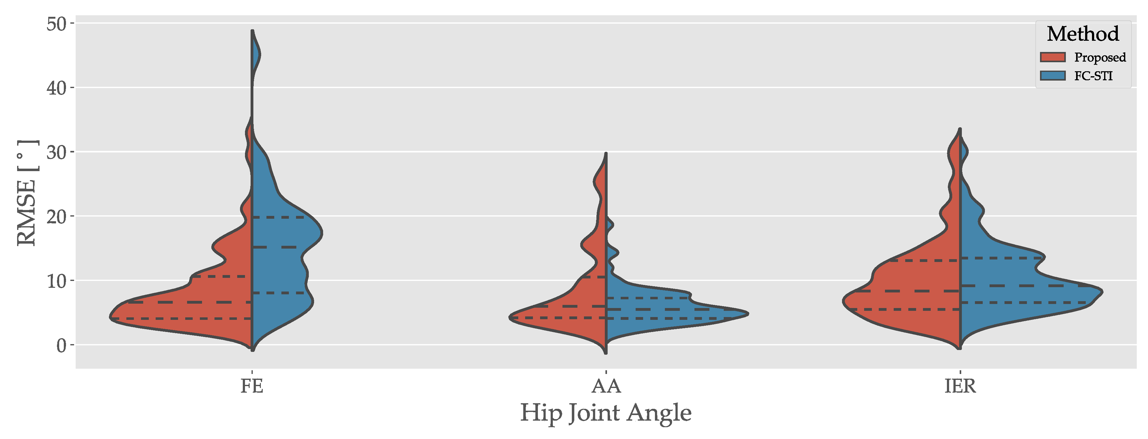
3.2. Joint Angles
4. Discussion
5. Conclusions
Author Contributions
Funding
Acknowledgments
Conflicts of Interest
References
- Constantinou, M.; Loureiro, A.; Carty, C.; Mills, P.; Barrett, R. Hip joint mechanics during walking in individuals with mild-to-moderate hip osteoarthritis. Gait Posture 2017, 53, 162–167. [Google Scholar] [CrossRef] [PubMed]
- Huisinga, J.M.; Schmid, K.K.; Filipi, M.L.; Stergiou, N. Gait Mechanics Are Different between Healthy Controls and Patients with Multiple Sclerosis. J. Appl. Biomech. 2013, 29, 303–311. [Google Scholar] [CrossRef] [PubMed]
- Morris, M.; Iansek, R.; McGinley, J.; Matyas, T.; Huxham, F. Three-dimensional gait biomechanics in Parkinson’s disease: Evidence for a centrally mediated amplitude regulation disorder. Mov. Disord. 2005, 20, 40–50. [Google Scholar] [CrossRef] [PubMed]
- Laudanski, A.; Brouwer, B.; Li, Q. Measurement of Lower Limb Joint Kinematics using Inertial Sensors During Stair Ascent and Descent in Healthy Older Adults and Stroke Survivors. J. Healthc. Eng. 2013, 4, 555–576. [Google Scholar] [CrossRef]
- Kvist, J. Rehabilitation Following Anterior Cruciate Ligament Injury: Current Recommendations for Sports Participation. Sport. Med. 2004, 34, 269–280. [Google Scholar] [CrossRef]
- Della Villa, S.; Boldrini, L.; Ricci, M.; Danelon, F.; Snyder-Mackler, L.; Nanni, G.; Roi, G.S. Clinical Outcomes and Return-to-Sports Participation of 50 Soccer Players After Anterior Cruciate Ligament Reconstruction Through a Sport-Specific Rehabilitation Protocol. Sport. Health 2012, 4, 17–24. [Google Scholar] [CrossRef]
- Motta, C.; Palermo, E.; Studer, V.; Germanotta, M.; Germani, G.; Centonze, D.; Cappa, P.; Rossi, S.; Rossi, S. Disability and Fatigue Can Be Objectively Measured in Multiple Sclerosis. PLoS ONE 2016, 11, e0148997. [Google Scholar] [CrossRef]
- Kerrigan, D.C.; Lee, L.W.; Collins, J.J.; Riley, P.O.; Lipsitz, L.A. Reduced hip extension during walking: Healthy elderly and fallers versus young adults. Arch. Phys. Med. Rehabil. 2001, 82, 26–30. [Google Scholar] [CrossRef]
- Shore, B.J.; Allar, B.; Miller, P.E.; Yen, Y.M.; Matheney, T.H.; Kim, Y.J. Childhood Obesity: Adverse Effects on Activity and Hip Range of Motion. Orthop. J. Harv. Med. Sch. 2018, 19, 24–31. [Google Scholar]
- Cappozzo, A.; Dellacroce, U.; Leardini, A.; Chiari, L. Human movement analysis using stereophotogrammetry Part 1: theoretical background. Gait Posture 2005, 21, 186–196. [Google Scholar] [CrossRef]
- Fasel, B.; Spörri, J.; Schütz, P.; Lorenzetti, S.; Aminian, K. Validation of functional calibration and strap-down joint drift correction for computing 3D joint angles of knee, hip, and trunk in alpine skiing. PLoS ONE 2017, 12, e0181446. [Google Scholar] [CrossRef] [PubMed]
- Fasel, B.; Spörri, J.; Schütz, P.; Lorenzetti, S.; Aminian, K. An Inertial Sensor-Based Method for Estimating the Athlete’s Relative Joint Center Positions and Center of Mass Kinematics in Alpine Ski Racing. Front. Physiol. 2017, 8. [Google Scholar] [CrossRef] [PubMed]
- Fasel, B.; Sporri, J.; Chardonnens, J.; Kroll, J.; Muller, E.; Aminian, K. Joint Inertial Sensor Orientation Drift Reduction for Highly Dynamic Movements. IEEE J. Biomed. Health Inform. 2018, 22, 77–86. [Google Scholar] [CrossRef] [PubMed]
- Seel, T.; Raisch, J.; Schauer, T. IMU-Based Joint Angle Measurement for Gait Analysis. Sensors 2014, 14, 6891–6909. [Google Scholar] [CrossRef]
- Seel, T.; Schauer, T.; Raisch, J. Joint axis and position estimation from inertial measurement data by exploiting kinematic constraints. In Proceedings of the 2012 IEEE International Conference on Control Applications, Dubrovnik, Croatia, 3–5 October 2012; IEEE: Dubrovnik, Croatia, 2012; pp. 45–49. [Google Scholar] [CrossRef]
- Vitali, R.; Cain, S.; McGinnis, R.; Zaferiou, A.; Ojeda, L.; Davidson, S.; Perkins, N. Method for Estimating Three-Dimensional Knee Rotations Using Two Inertial Measurement Units: Validation with a Coordinate Measurement Machine. Sensors 2017, 17, 1970. [Google Scholar] [CrossRef]
- El-Gohary, M.; McNames, J. Shoulder and Elbow Joint Angle Tracking With Inertial Sensors. IEEE Trans. Biomed. Eng. 2012, 59, 2635–2641. [Google Scholar] [CrossRef]
- El-Gohary, M.; McNames, J. Human Joint Angle Estimation with Inertial Sensors and Validation with A Robot Arm. IEEE Trans. Biomed. Eng. 2015, 62, 1759–1767. [Google Scholar] [CrossRef]
- Muller, P.; Begin, M.A.; Schauer, T.; Seel, T. Alignment-Free, Self-Calibrating Elbow Angles Measurement Using Inertial Sensors. IEEE J. Biomed. Health Inform. 2017, 21, 312–319. [Google Scholar] [CrossRef]
- Lebel, K.; Boissy, P.; Nguyen, H.; Duval, C. Inertial measurement systems for segments and joints kinematics assessment: Towards an understanding of the variations in sensors accuracy. Biomed. Eng. Online 2017, 16. [Google Scholar] [CrossRef]
- Bolink, S.; Naisas, H.; Senden, R.; Essers, H.; Heyligers, I.; Meijer, K.; Grimm, B. Validity of an inertial measurement unit to assess pelvic orientation angles during gait, sit—Stand transfers and step-up transfers: Comparison with an optoelectronic motion capture system. Med. Eng. Phys. 2016, 38, 225–231. [Google Scholar] [CrossRef]
- Won, S.h.P.; Melek, W.W.; Golnaraghi, F. A Kalman/Particle Filter-Based Position and Orientation Estimation Method Using a Position Sensor/Inertial Measurement Unit Hybrid System. IEEE Trans. Ind. Electron. 2010, 57, 1787–1798. [Google Scholar] [CrossRef]
- Mazzà, C.; Donati, M.; McCamley, J.; Picerno, P.; Cappozzo, A. An optimized Kalman filter for the estimate of trunk orientation from inertial sensors data during treadmill walking. Gait Posture 2012, 35, 138–142. [Google Scholar] [CrossRef] [PubMed]
- Luinge, H.J.; Veltink, P.H. Measuring orientation of human body segments using miniature gyroscopes and accelerometers. Med. Biol. Eng. Comput. 2005, 43, 273–282. [Google Scholar] [CrossRef] [PubMed]
- Favre, J.; Jolles, B.; Siegrist, O.; Aminian, K. Quaternion-based fusion of gyroscopes and accelerometers to improve 3D angle measurement. Electron. Lett. 2006, 42, 612. [Google Scholar] [CrossRef]
- Cooper, G.; Sheret, I.; McMillian, L.; Siliverdis, K.; Sha, N.; Hodgins, D.; Kenney, L.; Howard, D. Inertial sensor-based knee flexion/extension angle estimation. J. Biomech. 2009, 42, 2678–2685. [Google Scholar] [CrossRef] [PubMed]
- McGinnis, R.S.; Cain, S.M.; Tao, S.; Whiteside, D.; Goulet, G.C.; Gardner, E.C.; Bedi, A.; Perkins, N.C. Accuracy of Femur Angles Estimated by IMUs During Clinical Procedures Used to Diagnose Femoroacetabular Impingement. IEEE Trans. Biomed. Eng. 2015, 62, 1503–1513. [Google Scholar] [CrossRef]
- McGinnis, R.S.; Patel, S.; Silva, I.; Mahadevan, N.; DiCristofaro, S.; Jortberg, E.; Ceruolo, M.; Aranyosi, A.J. Skin mounted accelerometer system for measuring knee range of motion. In Proceedings of the 2016 38th Annual International Conference of the IEEE Engineering in Medicine and Biology Society (EMBC), Orlando, FL, USA, 16–20 August 2016; pp. 5298–5302. [Google Scholar] [CrossRef]
- McGinnis, R.S.; Cain, S.M.; Davidson, S.P.; Vitali, R.V.; McLean, S.G.; Perkins, N.C. Validation of Complementary Filter Based IMU Data Fusion for Tracking Torso Angle and Rifle Orientation. In Biomedical and Biotechnology Engineering; ASME: Montreal, QC, Canada, 2014; Volume 3, p. V003T03A052. [Google Scholar] [CrossRef]
- Zihajehzadeh, S.; Loh, D.; Lee, M.; Hoskinson, R.; Park, E.J. A cascaded two-step Kalman filter for estimation of human body segment orientation using MEMS-IMU. In Proceedings of the 2014 36th Annual International Conference of the IEEE Engineering in Medicine and Biology Society, Chicago, IL, USA, 26–30 August 2014; IEEE: Chicago, IL, USA, 2014; pp. 6270–6273. [Google Scholar] [CrossRef]
- Robert-Lachaine, X.; Mecheri, H.; Larue, C.; Plamondon, A. Validation of inertial measurement units with an optoelectronic system for whole-body motion analysis. Med. Biol. Eng. Comput. 2017, 55, 609–619. [Google Scholar] [CrossRef]
- Horenstein, R.E.; Lewis, C.L.; Yan, S.; Halverstadt, A.; Shefelbine, S.J. Validation of Magneto-Inertial Measuring Units for Measuring Hip Joint Angles. J. Biomech. 2019, 91, 170–174. [Google Scholar] [CrossRef]
- Madgwick, S.O.H.; Harrison, A.J.L.; Vaidyanathan, R. Estimation of IMU and MARG orientation using a gradient descent algorithm. In Proceedings of the 2011 IEEE International Conference on Rehabilitation Robotics, Zurich, Switzerland, 29 June–1 July 2011; pp. 1–7. [Google Scholar] [CrossRef]
- Ahmed, H.; Tahir, M. Improving the Accuracy of Human Body Orientation Estimation With Wearable IMU Sensors. IEEE Trans. Instrum. Meas. 2017, 66, 535–542. [Google Scholar] [CrossRef]
- Nüesch, C.; Roos, E.; Pagenstert, G.; Mündermann, A. Measuring joint kinematics of treadmill walking and running: Comparison between an inertial sensor based system and a camera-based system. J. Biomech. 2017, 57, 32–38. [Google Scholar] [CrossRef]
- Camomilla, V.; Cereatti, A.; Vannozzi, G.; Cappozzo, A. An optimized protocol for hip joint centre determination using the functional method. J. Biomech. 2006, 39, 1096–1106. [Google Scholar] [CrossRef] [PubMed]
- Wu, G.; Siegler, S.; Allard, P.; Kirtley, C.; Leardini, A.; Rosenbaum, D.; Whittle, M.; D’Lima, D.D.; Cristofolini, L.; Witte, H.; et al. ISB recommendation on definitions of joint coordinate system of various joints for the reporting of human joint motion—Part I: Ankle, hip, and spine. J. Biomech. 2002, 35, 543–548. [Google Scholar] [CrossRef]
- Ren, L.; Jones, R.K.; Howard, D. Whole body inverse dynamics over a complete gait cycle based only on measured kinematics. J. Biomech. 2008, 41, 2750–2759. [Google Scholar] [CrossRef] [PubMed]
- Camomilla, V.; Bonci, T.; Dumas, R.; Chèze, L.; Cappozzo, A. A model of the soft tissue artefact rigid component. J. Biomech. 2015, 48, 1752–1759. [Google Scholar] [CrossRef] [PubMed]
- Challis, J.H. A procedure for determining rigid body transformation parameters. J. Biomech. 1995, 28, 733–737. [Google Scholar] [CrossRef]
- Gamage, S.S.U.; Lasenby, J. New least squares solutions for estimating the average centre of rotation and the axis of rotation. J. Biomech. 2002, 35, 87–93. [Google Scholar] [CrossRef]
- Halvorsen, K. Bias compensated least squares estimate of the center of rotation. J. Biomech. 2003, 36, 999–1008. [Google Scholar] [CrossRef]
- Dabirrahmani, D.; Hogg, M. Modification of the Grood and Suntay Joint Coordinate System equations for knee joint flexion. Med. Eng. Phys. 2017, 39, 113–116. [Google Scholar] [CrossRef]
- Kalman, R.E. A New Approach to Linear Filtering and Prediction Problems. J. Basic Eng. 1960, 82, 35–45. [Google Scholar] [CrossRef]
- Kim, P. Kalman Filter for Beginners: With MATLAB Examples; CreateSpace Independent Publishing Platform: Scotts Valley, CA, USA, 2011. [Google Scholar]
- Zhao, S. Time Derivative of Rotation Matrices: A Tutorial. arXiv 2016, arXiv:1609.06088. [Google Scholar]
- Graf, B. Quaternions and dynamics. arXiv 2008, arXiv:0811.2889. [Google Scholar]
- McGinnis, R.S.; Perkins, N.C. Inertial sensor based method for identifying spherical joint center of rotation. J. Biomech. 2013, 46, 2546–2549. [Google Scholar] [CrossRef] [PubMed]
- Crabolu, M.; Pani, D.; Raffo, L.; Conti, M.; Crivelli, P.; Cereatti, A. In vivo estimation of the shoulder joint center of rotation using magneto-inertial sensors: MRI-based accuracy and repeatability assessment. BioMed. Eng. OnLine 2017, 16. [Google Scholar] [CrossRef] [PubMed]
- Sabatini, A.M. Kalman-Filter-Based Orientation Determination Using Inertial/Magnetic Sensors: Observability Analysis and Performance Evaluation. Sensors 2011, 11, 9182–9206. [Google Scholar] [CrossRef] [PubMed]


| Trial | Method | RMSE () | Slope | Intercept () |
|---|---|---|---|---|
| Star Calibration | SSRO | 12.32 (13.89) | 0.91 (0.18) | 14.51 (30.07) |
| APDM | 24.61 (18.59) | 0.85 (0.51) | 21.91 (71.24) | |
| Walking | SSRO | 11.82 (11.53) | 0.95 (0.17) | 8.10 (26.81) |
| APDM | 23.76 (21.61) | 0.85 (0.51) | 22.07 (63.78) |
| Trial | Method | Angle | RMSE () | Slope | Intercept () | ROMD () | Drift (/s) |
|---|---|---|---|---|---|---|---|
| Star Calibration | Proposed | FE | 7.88 (3.64) | 1.04 (0.09) | −2.91 (6.48) | 18.08 (12.57) | - |
| AA | 9.16 (6.69) | 0.98 (0.21) | −5.45 (7.45) | 8.74 (14.93) | - | ||
| IER | 10.36 (7.04) | 0.90 (0.56) | −2.53 (9.79) | 10.21 (14.33) | - | ||
| FC-STI | FE | 14.49 (6.28) | 1.04 (0.07) | −4.48 (14.20) | 16.35 (12.38) | - | |
| AA | 6.24 (2.61) | 0.96 (0.18) | −2.21 (4.22) | 3.13 (10.34) | - | ||
| IER | 8.96 (3.90) | 0.95 (0.33) | −4.12 (7.46) | 4.58 (7.69) | - | ||
| Walking | Proposed | FE | 8.62 (7.52) | 1.00 (0.07) | −6.29 (9.15) | 2.17 (3.61) | −0.00 (0.03) |
| AA | 8.03 (6.42) | 0.94 (0.12) | −3.93 (9.00) | 0.80 (4.64) | 0.01 (0.02) | ||
| IER | 9.99 (5.90) | 0.78 (0.31) | −5.92 (8.69) | 0.77 (4.34) | −0.03 (0.07) | ||
| FC-STI | FE | 15.64 (10.24) | 0.97 (0.06) | −10.17 (14.75) | 1.86 (3.44) | −0.01 (0.03) | |
| AA | 5.65 (3.16) | 0.95 (0.12) | −1.97 (5.07) | 3.35 (5.55) | 0.03 (0.06) | ||
| IER | 11.93 (6.04) | 0.76 (0.22) | 6.19 (1.28) | 4.49 (6.78) | −0.12 (0.18) |
© 2019 by the authors. Licensee MDPI, Basel, Switzerland. This article is an open access article distributed under the terms and conditions of the Creative Commons Attribution (CC BY) license (http://creativecommons.org/licenses/by/4.0/).
Share and Cite
Adamowicz, L.; Gurchiek, R.D.; Ferri, J.; Ursiny, A.T.; Fiorentino, N.; McGinnis, R.S. Validation of Novel Relative Orientation and Inertial Sensor-to-Segment Alignment Algorithms for Estimating 3D Hip Joint Angles. Sensors 2019, 19, 5143. https://doi.org/10.3390/s19235143
Adamowicz L, Gurchiek RD, Ferri J, Ursiny AT, Fiorentino N, McGinnis RS. Validation of Novel Relative Orientation and Inertial Sensor-to-Segment Alignment Algorithms for Estimating 3D Hip Joint Angles. Sensors. 2019; 19(23):5143. https://doi.org/10.3390/s19235143
Chicago/Turabian StyleAdamowicz, Lukas, Reed D. Gurchiek, Jonathan Ferri, Anna T. Ursiny, Niccolo Fiorentino, and Ryan S. McGinnis. 2019. "Validation of Novel Relative Orientation and Inertial Sensor-to-Segment Alignment Algorithms for Estimating 3D Hip Joint Angles" Sensors 19, no. 23: 5143. https://doi.org/10.3390/s19235143
APA StyleAdamowicz, L., Gurchiek, R. D., Ferri, J., Ursiny, A. T., Fiorentino, N., & McGinnis, R. S. (2019). Validation of Novel Relative Orientation and Inertial Sensor-to-Segment Alignment Algorithms for Estimating 3D Hip Joint Angles. Sensors, 19(23), 5143. https://doi.org/10.3390/s19235143