Fabrication, Measurement and Time Decay of the Electromagnetic Properties of Semi-Solid Water-Based Phantoms


Abstract
:1. Introduction
2. Homogeneous Phantom Fabrication
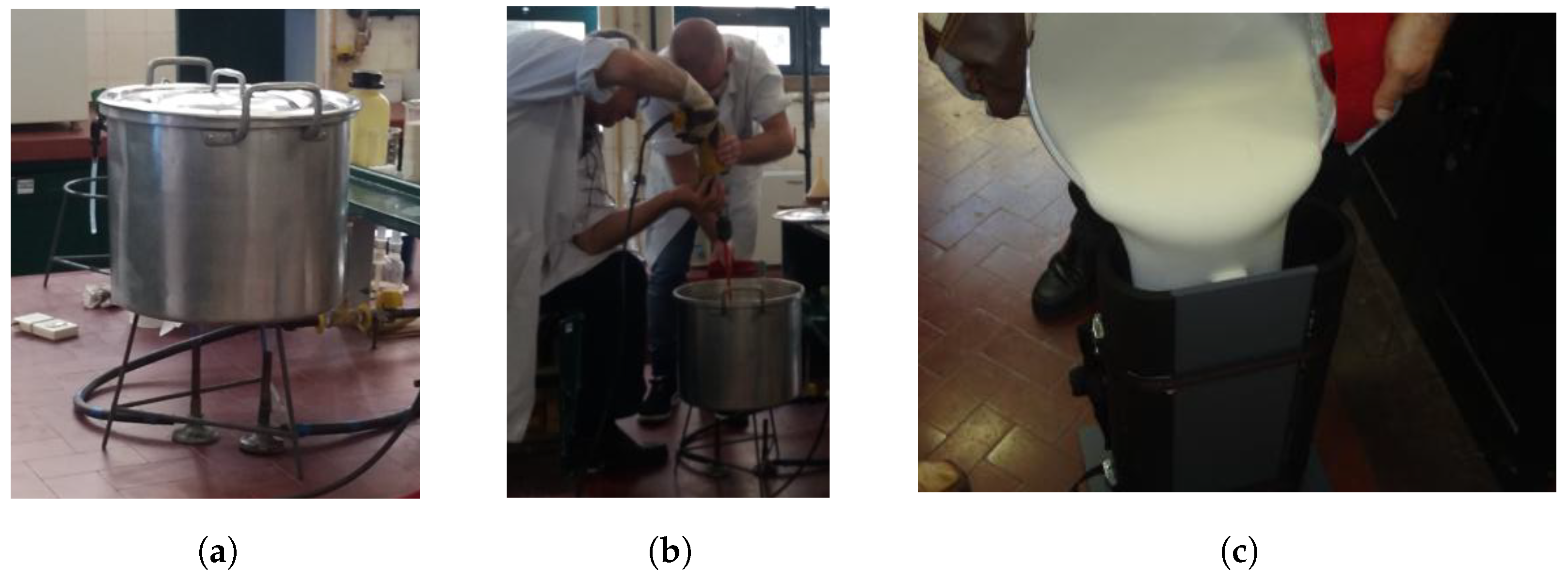
- Deionized water is placed on a kettle and heated on a gas burner. During the heating process, sodium chloride and sodium azide are added to the water. To prevent evaporation, the heating process must be performed with the kettle’s lid on.
- Once the water starts to reach the boiling point, agar is slowly added and dissolved.
- When the mixture reaches the boiling point, fire is extinguished immediately.
- Small quantities of TX-151 and polyethylene powder are sprinkled into the liquid several times and quickly mixed with an electrical mixer at a speed fast enough to assure a uniform mixture but not so fast that air bubbles are formed.
- After all ingredients are added, the mixture is poured into the container, which must be immediately closed (with a plastic lid or cling-film) to prevent evaporation.
- Finally, the mixture is allowed to completely cool down to room temperature (for about a day) to completely solidify. After that period, the phantom can be removed from the container but must be kept in a hermetical environment to reduce water evaporation.
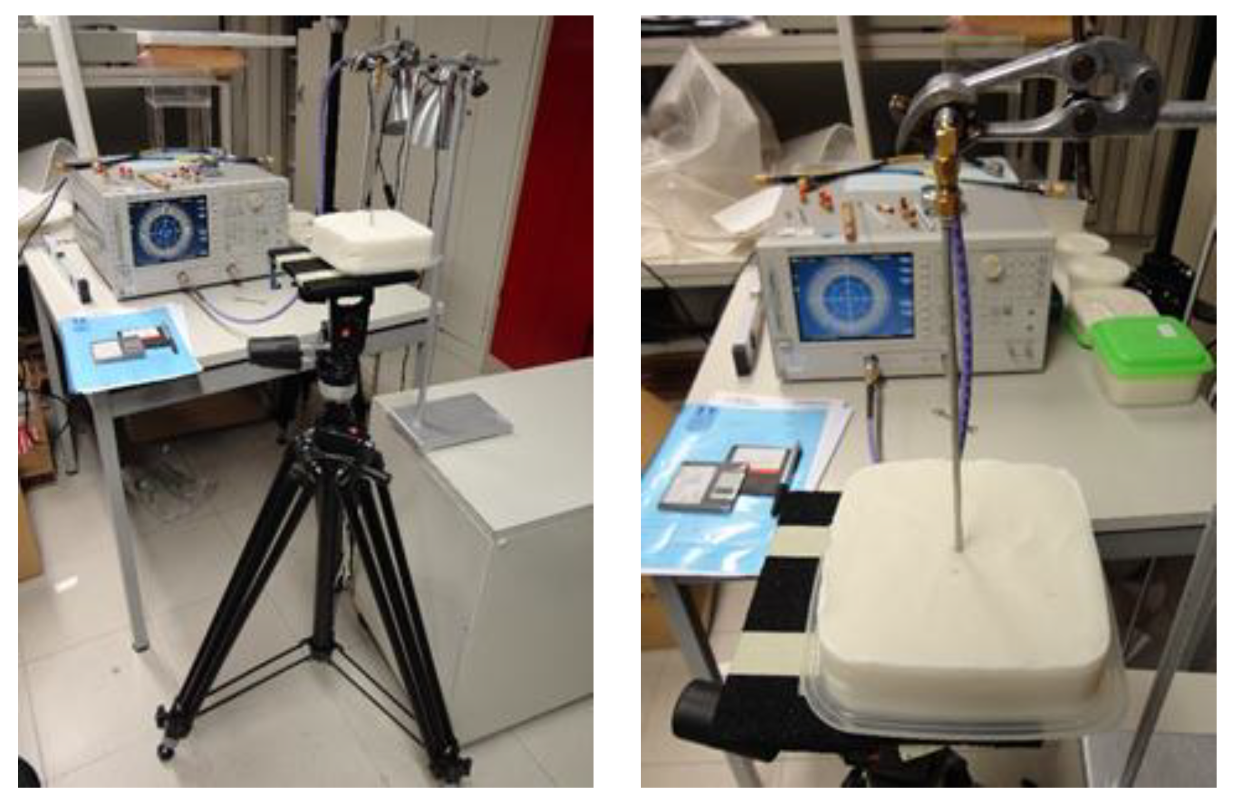
3. Measurement Technique
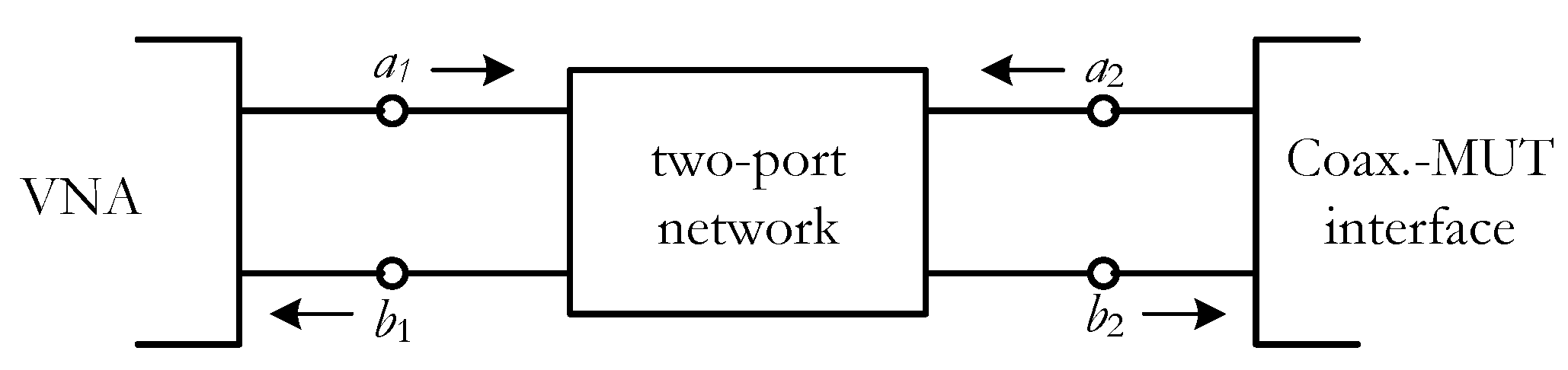
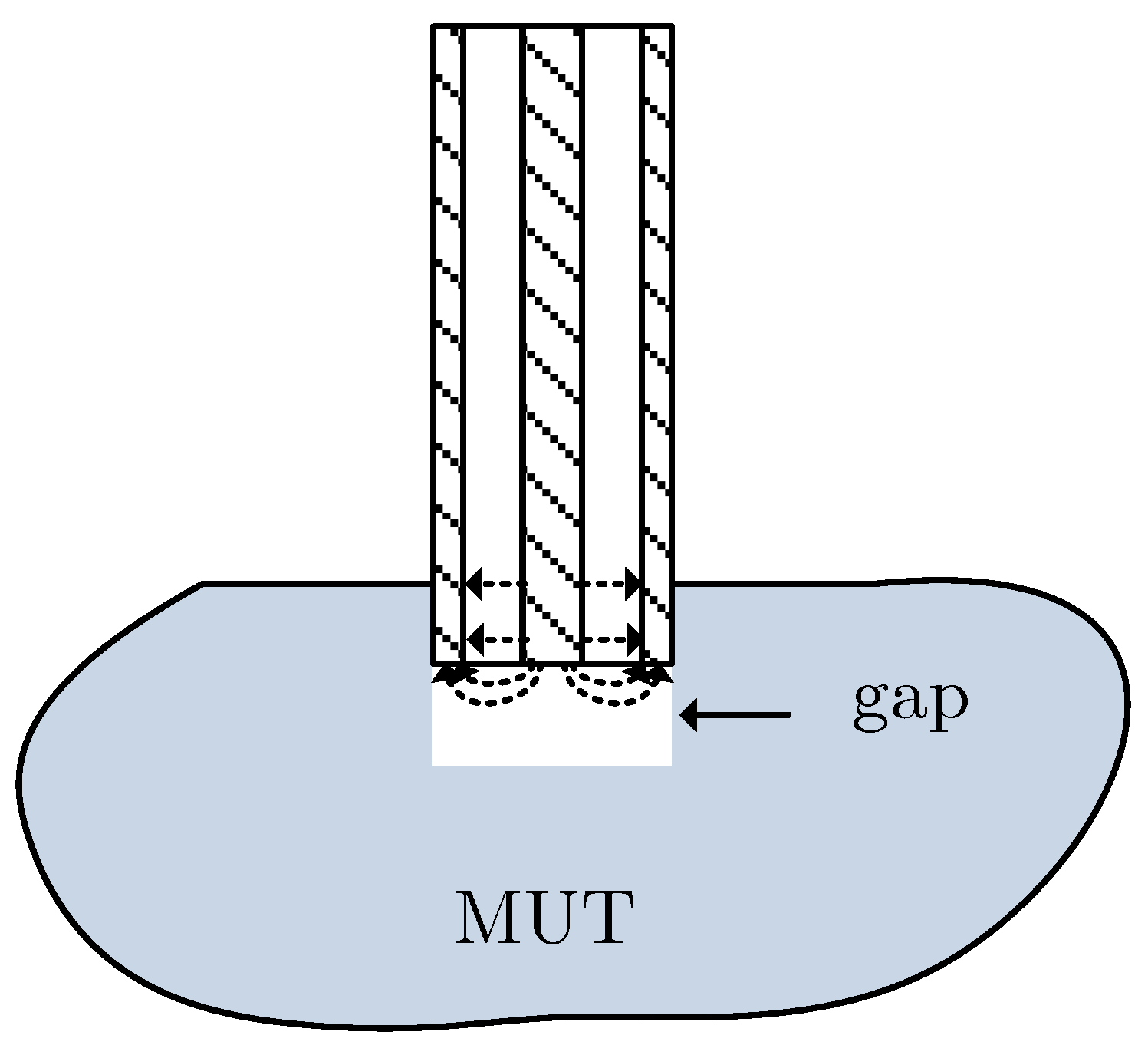
3.1. Method Description
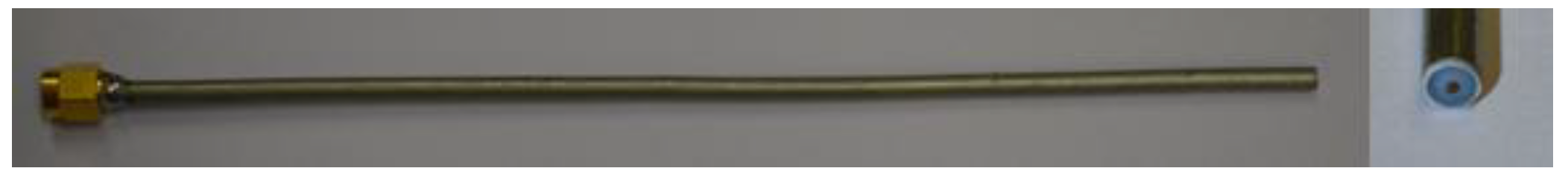
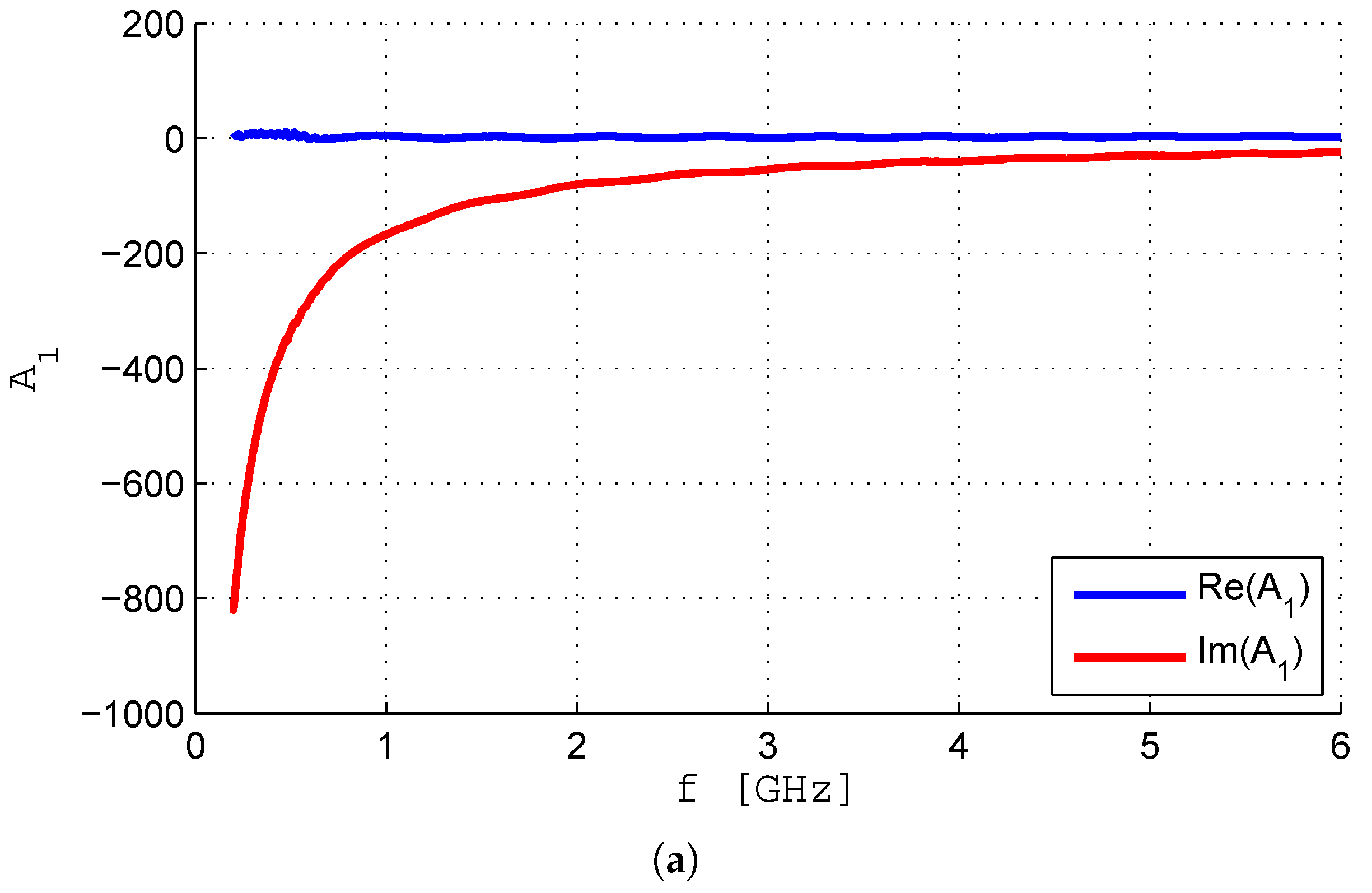
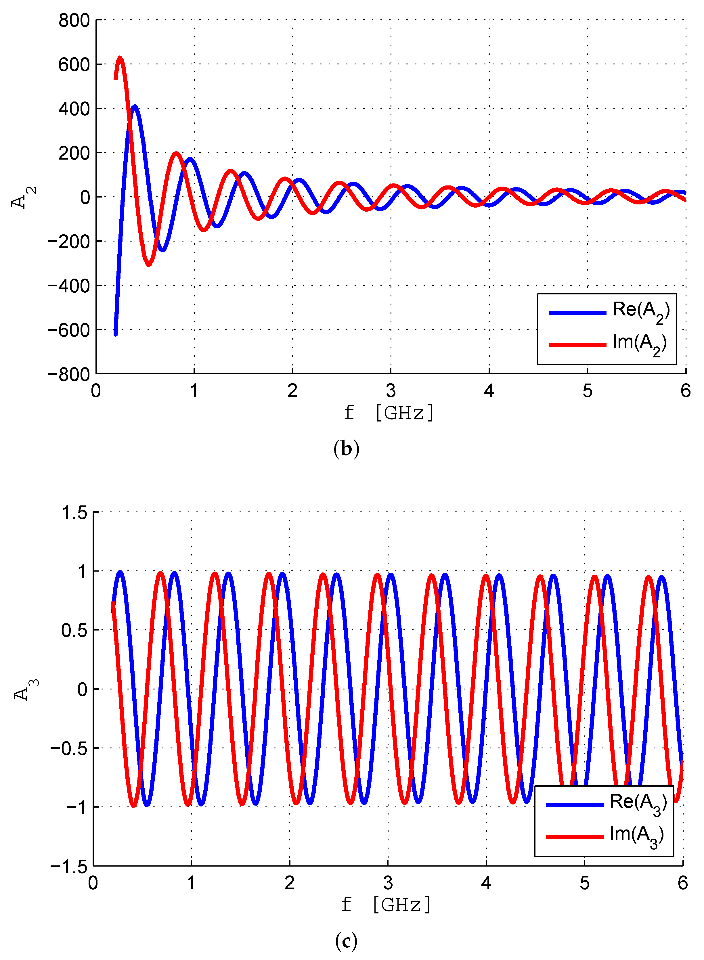
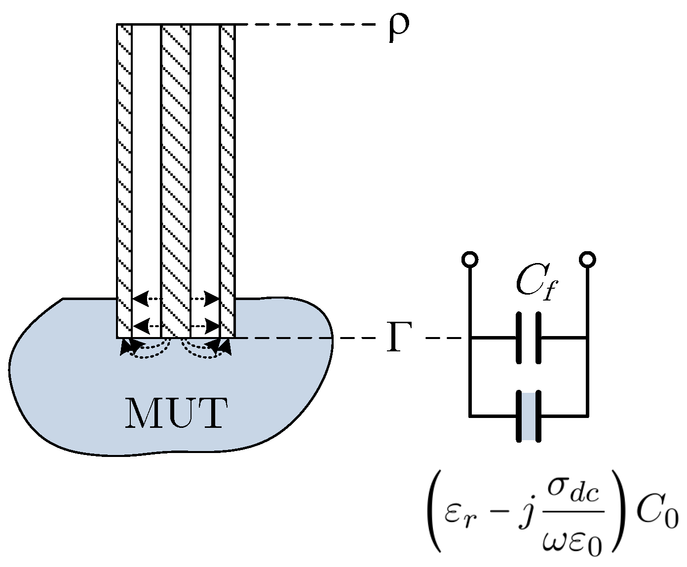
3.2. Coaxial Probe Description
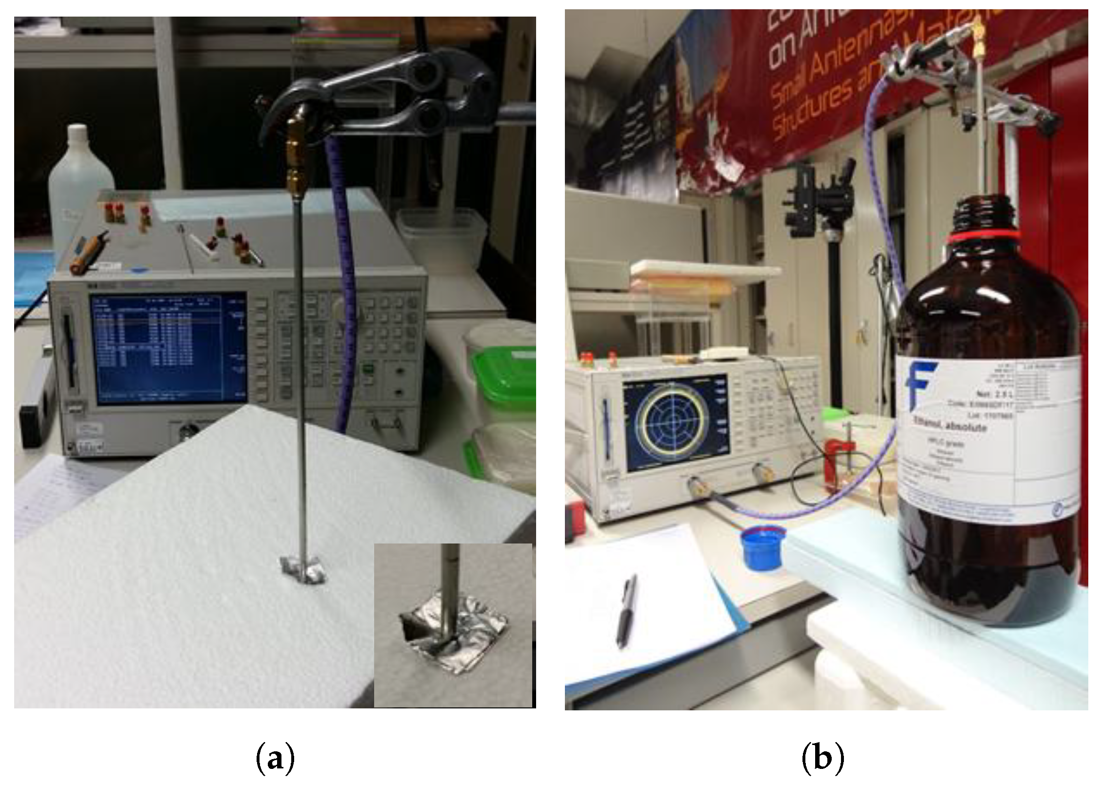
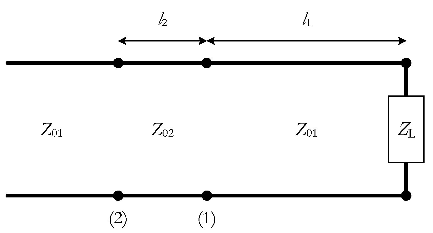
3.3. Coaxial Probe Calibration
4. Phantom Measurements
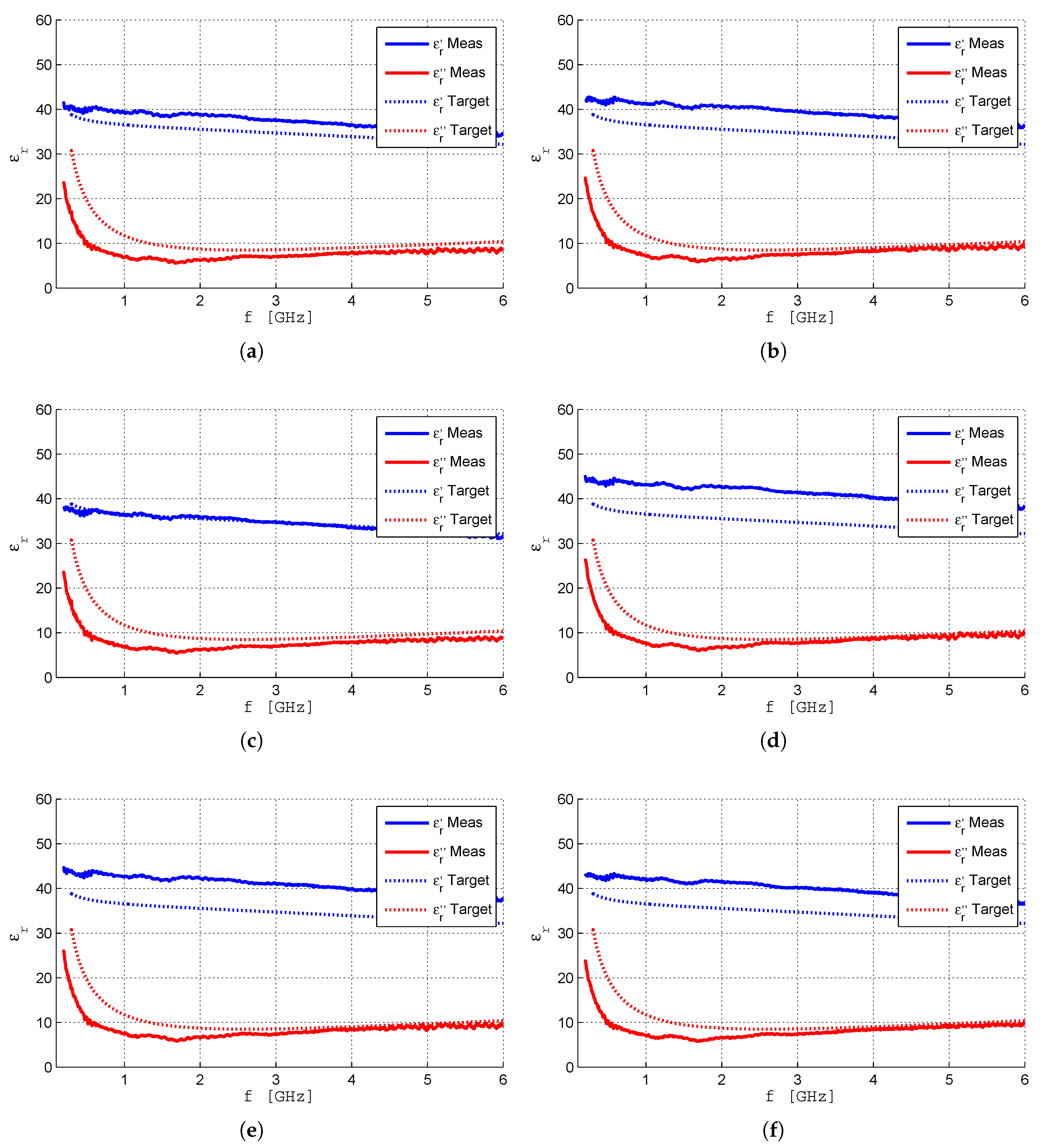
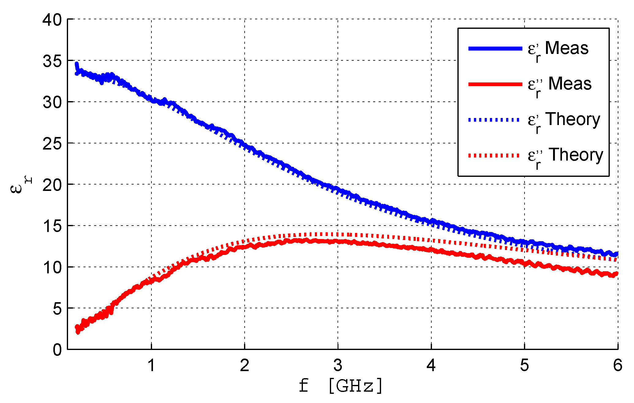
4.1. Comparison between Measured and Target Permittivity
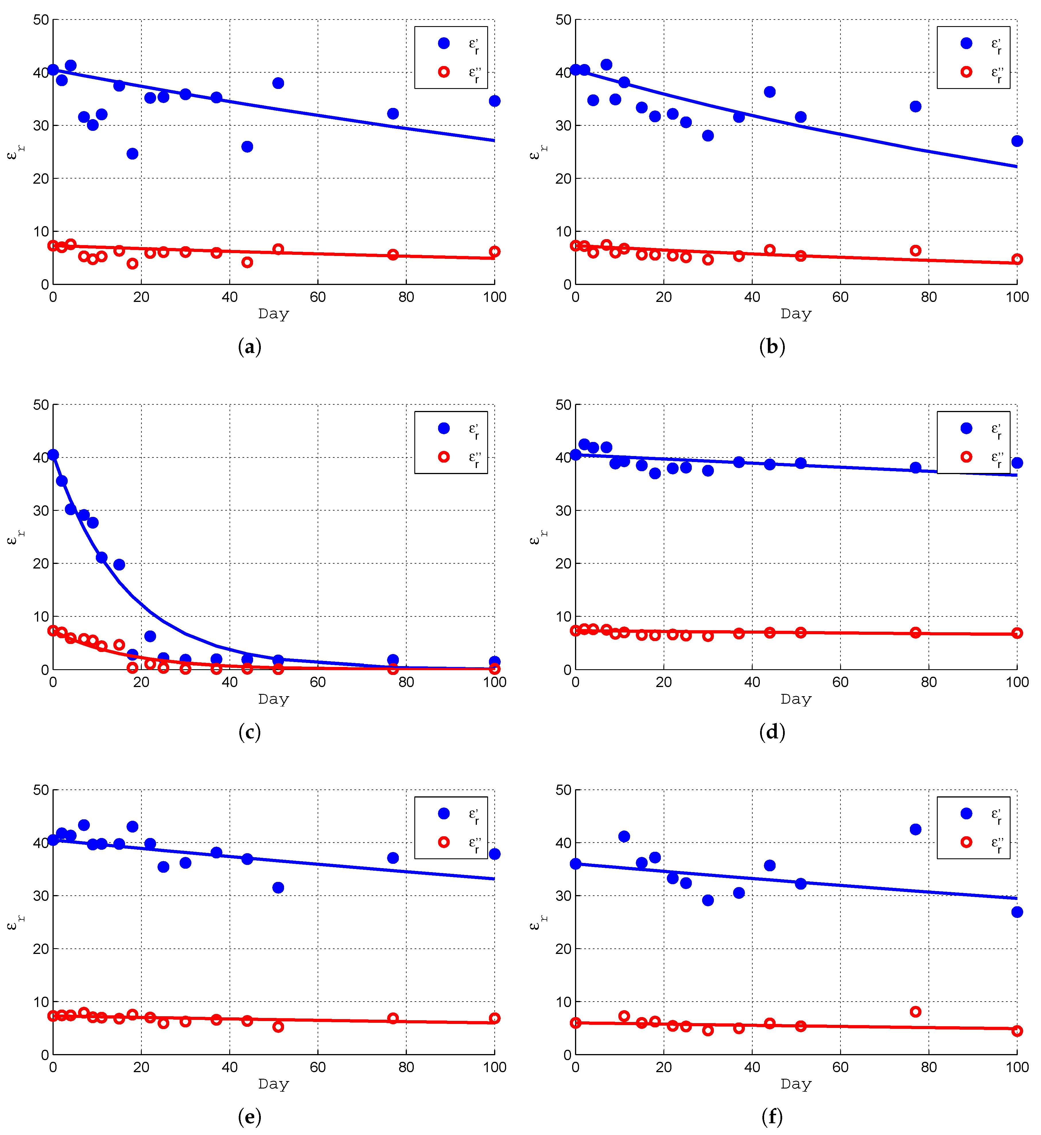
4.2. Time Evolution of the Phantom’s Characteristics
- Except for sample 3 (unprotected) the time decaying of the permittivity is almost linear.
- The real part and the imaginary part of the permittivity have similar time decaying rates although a slightly faster decay of the imaginary part is noticed.
- The useful lifetime of an unprotected phantom is very small (a few days only).
- The most effective protection is a hermetic sealing box that can extend a phantom lifetime many months or even a year. This long extension of the lifetime is only possible if the volume of air is contact with the phantom is small and is not renewed.
- Wrapping a phantom in plastic film can also extend the useful lifetime of a phantom, not as much as a hermetic box, but it can reach up to a month.
5. Conclusions
Author Contributions
Funding
Conflicts of Interest
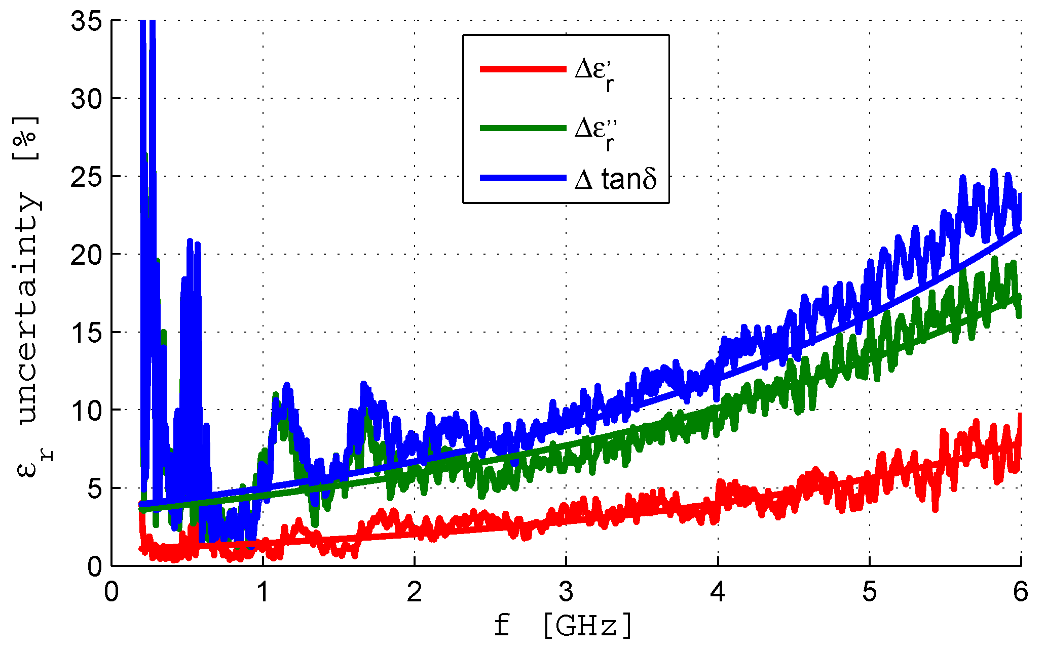
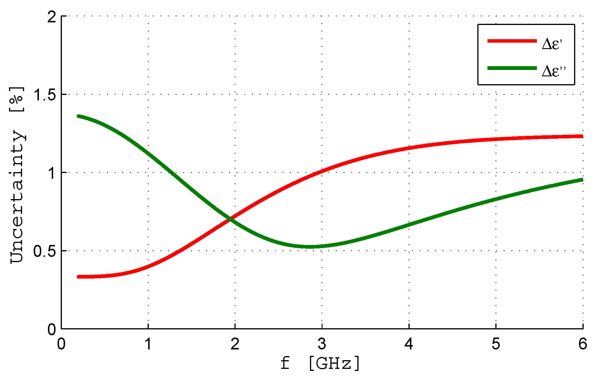
Appendix A. Coaxial Probe Uncertainty Analysis

| T (°C) | (ps) | ||
|---|---|---|---|
| 10 | |||
| 15 | |||
| 20 | |||
| 25 | |||
| 30 |

| Parameter | |||
|---|---|---|---|
| A | 1.0250 | 3.4302 | 3.717 |
| B | 0.3398 | 0.2701 | 0.293 |

References
- Mobashsher, A.; Abbosh, A. Artificial Human Phantoms: Human Proxy in Testing Microwave Apparatuses That Have Electromagnetic Interaction with the Human Body. IEEE Microw. Mag. 2015, 16, 42–62. [Google Scholar] [CrossRef]
- Mendes, C.; Peixeiro, C. A Dual-Mode Single-Band Wearable Microstrip Antenna for Body Area Networks. IEEE Antennas Wirel. Propag. Lett. 2017, 16, 3055–3058. [Google Scholar] [CrossRef]
- Mendes, C.; Peixeiro, C. On-Body Transmission Performance of a Novel Dual-Mode Wearable Microstrip Antenna. IEEE Trans. Antennas Propag. 2018, 66, 4872–4877. [Google Scholar] [CrossRef]
- Andreuccetti, D.; Fossi, R.; Petrucci, C. An Internet Resource for the Calculation of the Dielectric Properties of Body Tissues in the Frequency range 10 Hz–100 GHz. Available online: http://niremf.ifac.cnr.it/tissprop/ (accessed on 3 October 2019).
- Bringuier, J.; Mittra, R. Electromagnetic Wave Propagation in Body Area Networks Using the Finite- Difference-Time-Domain Method. Sensors 2012, 12, 9862–9883. [Google Scholar] [CrossRef] [PubMed]
- Fayos-Fernandez, J.; Arranz-Faz, C.; Martinez-Gonzalez, A.M.; Sanchez-Hernandez, D. Effect of pierced metallic objects on SAR distributions at 900 MHz. Bioelectromagnetics 2006, 27, 337–353. [Google Scholar] [CrossRef] [PubMed]
- Furse, C.M.; Chen, J.Y.; Gandhi, O.P. The use of the frequency-dependent finite-difference time-domain method for induced current and SAR calculations for a heterogeneous model of the human body. IEEE Trans. Electromagn. Comput. 1994, 36, 128–133. [Google Scholar] [CrossRef]
- Gandhi, O.P.; Gao, B.Q.; Chen, J.Y. A frequency-dependent finite-difference time-domain formulation for general dispersive media. IEEE Trans. Microw. Theory Tech. 1993, 41, 658–665. [Google Scholar] [CrossRef]
- Gabriel, C. Compilation of Dielectric Properties of Body Tissues at RF and Microwave Frequencies; Report N.AL/OE-TR- 1996-0037; Occupational and Environmental Health Directorate, Radiofrequency Radiation Division, Brooks Air Force Base: San Antonio, TX, USA, June 1996.
- Chou, C.K.; Chen, G.W.; Guy, A.W.; Luk, K.H. Formulas for preparing phantom muscle tissue at various radiofrequencies. Bioelectromagnetics 1984, 5, 435–441. [Google Scholar] [CrossRef] [PubMed]
- Hagmann, M.J.; Levin, R.L.; Calloway, L.; Osborn, A.J.; Foster, K.R. Muscle-equivalent phantom materials for 10–100 MHz. IEEE Trans. Microw. Theory Tech. 1992, 40, 760–762. [Google Scholar] [CrossRef]
- Ito, K.; Furuya, K.; Okano, Y.; Hamada, L. Development and characteristics of a biological tissue-equivalent phantom for microwaves. Electron. Commun. Jpn. Part I Commun. 2001, 84, 67–77. [Google Scholar] [CrossRef]
- Ito, K.; Kawai, H. Solid phantoms for evaluation of interactions between the human body and antennas. In Proceedings of the IEEE International Workshop on Antenna Technology: Small Antennas and Novel Metamaterials, Singapore, 7–9 March 2005; pp. 41–44. [Google Scholar]
- Ito, K. Human Body Phantoms for Evaluation of Wearable and Implantable Antennas. In Proceedings of the 2nd European Conference on Antennas and Propagation (EuCAP), Edinburgh, UK, 11–16 November 2007. [Google Scholar]
- Takimoto, T.; Onishi, T.; Saito, K.; Takahashi, M.; Uebayashi, S.; Ito, K. Evaluation on biological tissue equivalent Agar-based solid phantoms up to 10 GHz—Aiming at measurement of characteristics of antenna for UWB communications. In Proceedings of the International Symposium on Antennas and Propagation, Washington, DC, USA, 3–8 July 2005; pp. 483–486. [Google Scholar]
- Chahat, N.; Zhadobov, M.; Alekseev, S.; Sauleau, R. Human skin-equivalent phantom for on-body antenna measurements in 60 GHz band. Electron. Lett. 2012, 48, 67–68. [Google Scholar] [CrossRef]
- Chahat, N.; Zhadobov, M.; Sauleau, R. Skin-equivalent phantom for on-body antenna measurements at 60 GHz. In Proceedings of the 6th European Conference on Antennas and Propagation (EuCAP), Prague, Czech Republic, 26–30 March 2012; pp. 1362–1664. [Google Scholar]
- Chandra, R.; Johansson, A.J. Analytical model, measurements, and effect of outer lossless shell of phantoms for on-body propagation channel around the body for body area networks. In Proceedings of the 9th European Conference on Antennas and Propagation (EuCAP), Lisbon, Portugal, 13–17 April 2015. [Google Scholar]
- Stuchly, M.A.; Stuchly, S.S. Coaxial Line Reflection Methods for Measuring Dielectric Properties of Biological Substances at Radio and Microwave Frequencies-A Review. IEEE Trans. Instrum. Meas. 1980, 29, 176–183. [Google Scholar] [CrossRef]
- Stuchly, M.A.; Brady, M.M.; Stuchly, S.S.; Gajda, G. Equivalent circuit of an open-ended coaxial line in a lossy dielectric. IEEE Trans. Instrum. Meas. 1982, IM-31, 116–119. [Google Scholar] [CrossRef]
- Bobowski, J.S.; Johnson, T. Permittivity measurement of biological samples by an open-ended coaxial line. Prog. Electromagn. Res. B 2012, 38, 159–183. [Google Scholar] [CrossRef]
- Fornes-Leal, A.; Garcia-Pardo, C.; Cardona, N.; Castelló-Palacios, S.; Vallés-Lluch, A. Accurate broadband measurement of electromagnetic tissue phantoms using open-ended coaxial systems. In Proceedings of the 11th International Symposium on Medical Information and Communication Technology (ISMICT), Lisbon, Portugal, 6–8 February 2017; pp. 32–36. [Google Scholar]
- La Gioia, A.; Porter, E.; Merunka, I.; Shahzad, A.; Salahuddin, S.; Jones, M.; O’Halloran, M. Open-Ended Coaxial Probe Technique for Dielectric Measurement of Biological Tissues: Challenges and Common Practices. Diagnostics 2018, 8, 40. [Google Scholar] [CrossRef] [PubMed]
- Meaney, P.M.; Gregory, A.P.; Seppälä, J.; Lahtinen, T. Open-Ended Coaxial Dielectric Probe Effective Penetration Depth Determination. IEEE Trans. Microw. Theory Tech. 2016, 64, 915–923. [Google Scholar] [CrossRef] [PubMed]
- Kraszewski, A. (Ed.) Microwave Aquametry. Electromagnetic Wave Interaction with Water-Containing Materials; IEEE Press: New York, NY, USA, 1996. [Google Scholar]
- Gregory, A.P.; Clarke, R.N. Tables of the Complex Permittivity of Dielectric Reference Liquids at Frequencies up to 5 GHz; National Measurement System, Report MAT23; National Physical Laboratory: Teddington, UK, 2009.
- Kaatze, U. Measuring the dielectric properties of materials. Ninety-year development from low-frequency techniques to broadband spectroscopy and high-frequency imaging. Meas. Sci. Technol. 2013, 24, 1–31. [Google Scholar] [CrossRef]
- Nyshadham, A.; Sibbald, C.L.; Stuchly, S.S. Permittivity measurements using open-ended sensors and reference liquid calibration—An uncertainty analysis. IEEE Trans. Microw. Theory Tech. 1992, 40, 305–314. [Google Scholar] [CrossRef]


| Ingredient | Amount (g) | Amount (g) |
|---|---|---|
| (Original 4531.3 g) | (Scaled 12,000 g) | |
| Deionized water | 3375.0 | 8937.8 |
| Agar | 104.6 | 277.0 |
| Polyethylene powder | 1012.6 | 2681.6 |
| Sodium chloride | 7.0 | 18.5 |
| TX-151 | 30.1 | 79.7 |
| Sodium azide | 2.0 | 5.3 |
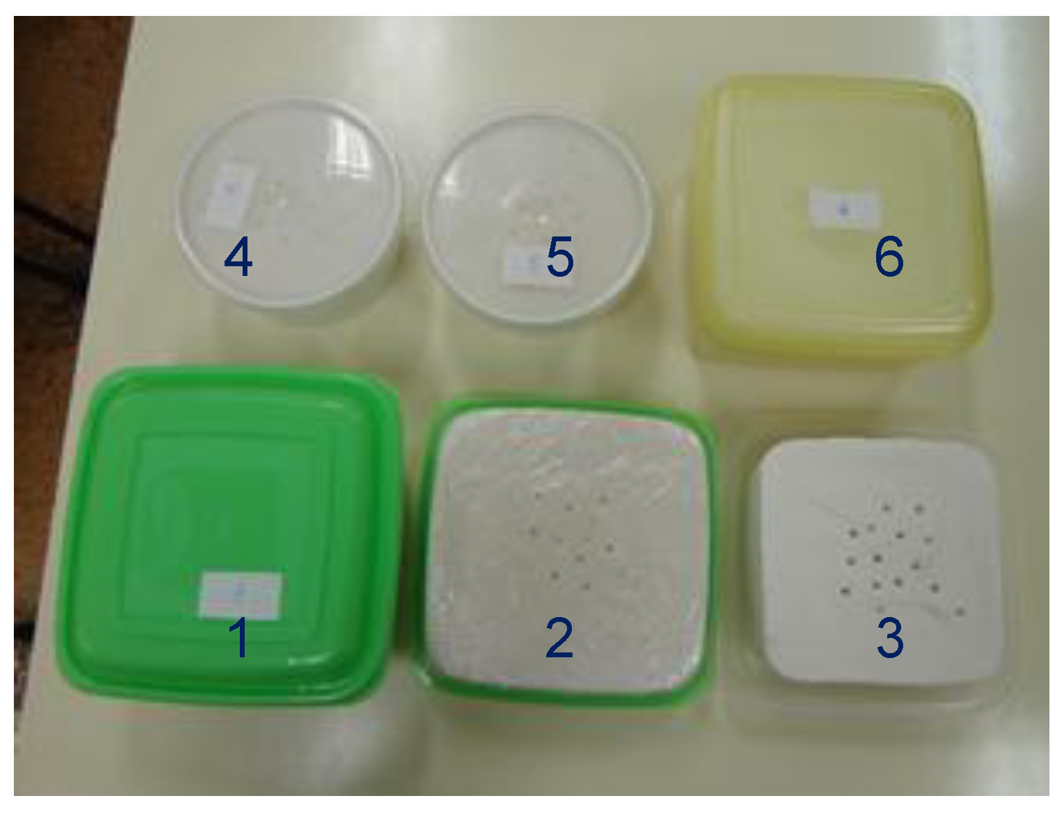
| Sample | Shape | Storage | Age | Dimensions | Air Gap |
|---|---|---|---|---|---|
| (cm) | (cm) | ||||
| 1 | parallelepiped | plastic box | recent | 13.5 × 13.5 × 5 | 3.5 |
| 2 | parallelepiped | cling-film | recent | 13.5 × 13.5 × 4 | 0 |
| 3 | parallelepiped | open | recent | 13.5 × 13.5 × 4 | - |
| 4 | cylindrical | plastic box | recent | 11 × 5.5 | 0.5 |
| 5 | cylindrical | plastic box | recent | 11 × 5.5 | 0.5 |
| 6 | parallelepiped | plastic box | 1 year | 13.5 × 13.5 × 6 | 1.0 |
| Frequency (GHz) | Attenuation Coefficient (dB/m) |
|---|---|
| 0.5 | 0.26 |
| 1 | 0.38 |
| 5 | 0.91 |
| 10 | 1.37 |
| 20 | 2.09 |
| Frequency (GHz) | Attenuation Coefficient (dB/m) |
|---|---|
| ≤5 | |
| ≥10 |
| Sample | ||
|---|---|---|
| 1 | 0.0039 | 0.0051 |
| 2 | 0.0050 | 0.0057 |
| 3 | 0.0700 | 0.0640 |
| 4 | 0.0010 | 0.0014 |
| 5 | 0.0016 | 0.0020 |
| 6 | 0.0036 | 0.0048 |
© 2019 by the authors. Licensee MDPI, Basel, Switzerland. This article is an open access article distributed under the terms and conditions of the Creative Commons Attribution (CC BY) license (http://creativecommons.org/licenses/by/4.0/).
Share and Cite
Mendes, C.; Peixeiro, C. Fabrication, Measurement and Time Decay of the Electromagnetic Properties of Semi-Solid Water-Based Phantoms. Sensors 2019, 19, 4298. https://doi.org/10.3390/s19194298
Mendes C, Peixeiro C. Fabrication, Measurement and Time Decay of the Electromagnetic Properties of Semi-Solid Water-Based Phantoms. Sensors. 2019; 19(19):4298. https://doi.org/10.3390/s19194298
Chicago/Turabian StyleMendes, Carlos, and Custódio Peixeiro. 2019. "Fabrication, Measurement and Time Decay of the Electromagnetic Properties of Semi-Solid Water-Based Phantoms" Sensors 19, no. 19: 4298. https://doi.org/10.3390/s19194298
APA StyleMendes, C., & Peixeiro, C. (2019). Fabrication, Measurement and Time Decay of the Electromagnetic Properties of Semi-Solid Water-Based Phantoms. Sensors, 19(19), 4298. https://doi.org/10.3390/s19194298