On the Application of Laser Vibrometry to Perform Structural Health Monitoring in Non-Stationary Conditions of a Hydropower Dam


Abstract
1. Introduction
2. Methods
Challenge for Non-Contact Vibration Monitoring during Full Operation of the Powerhouse
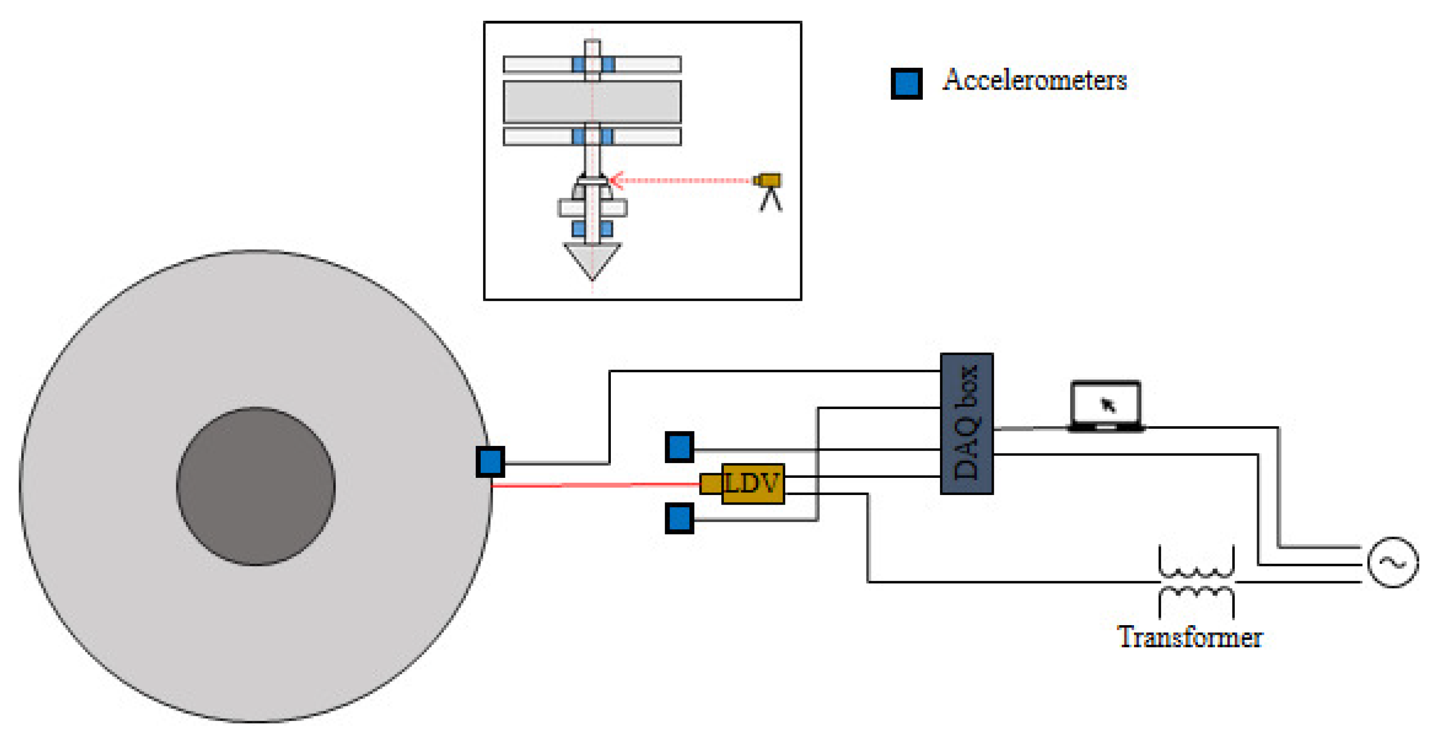
3. The Experiment
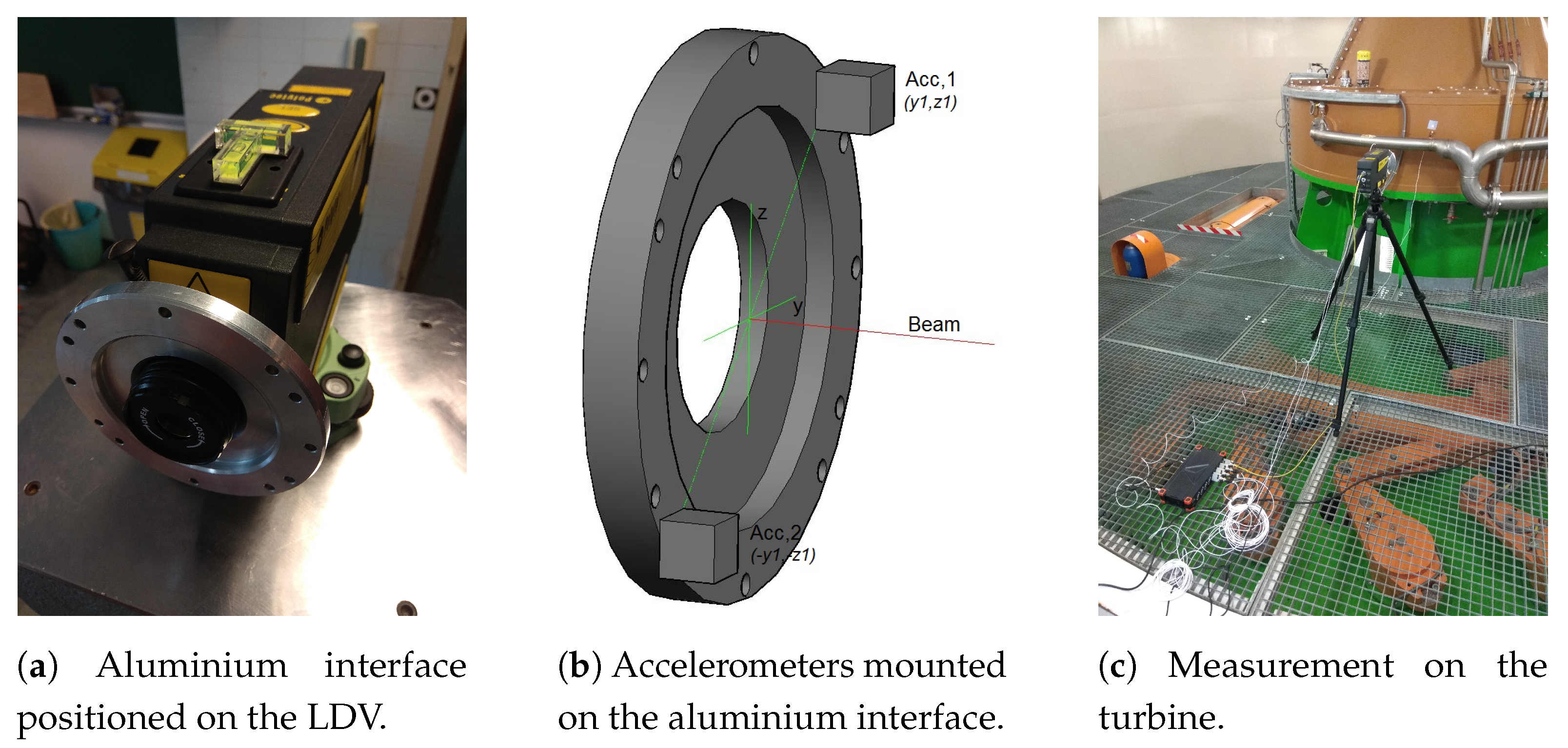
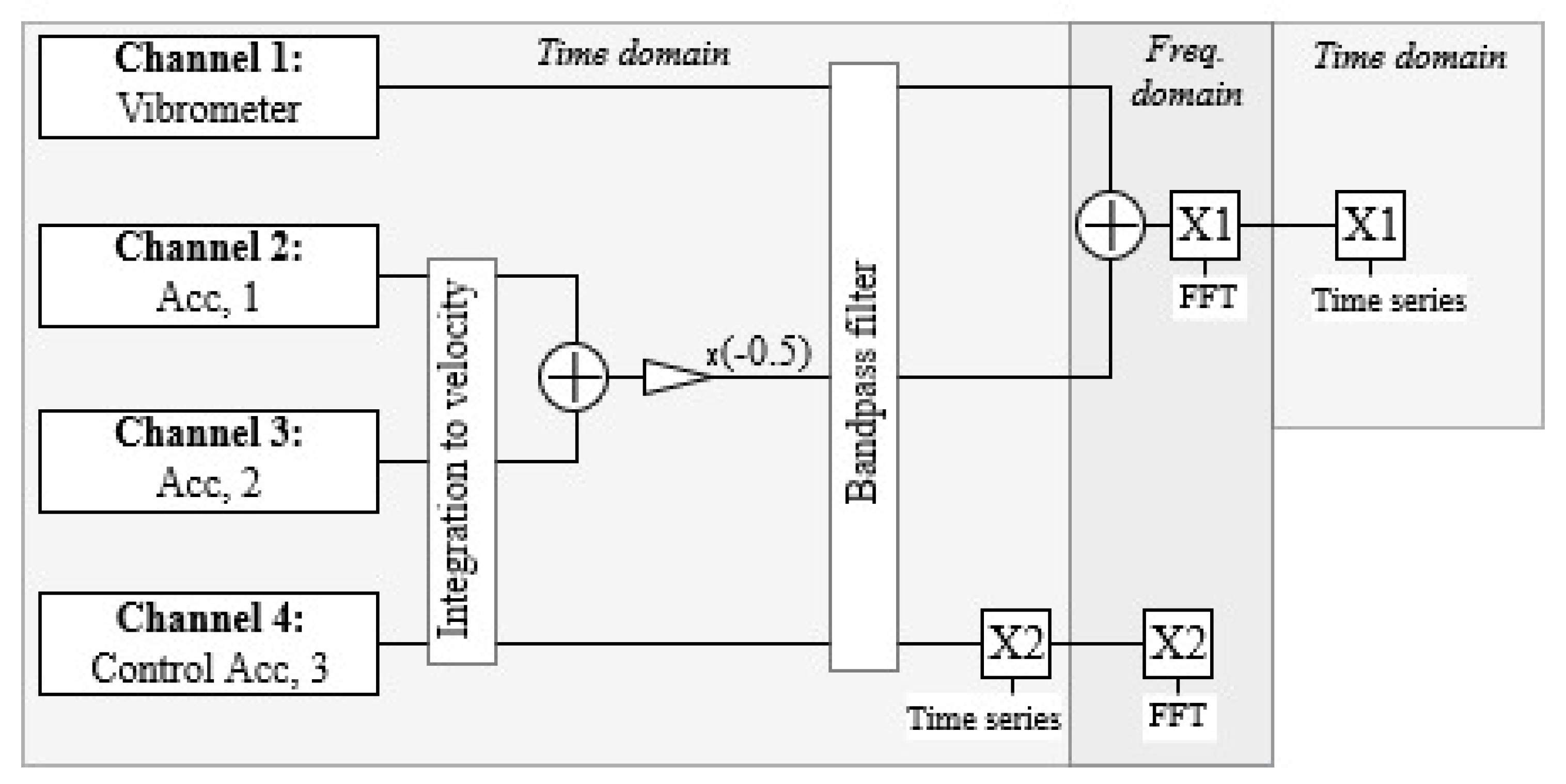
- Laser Doppler Vibrometer
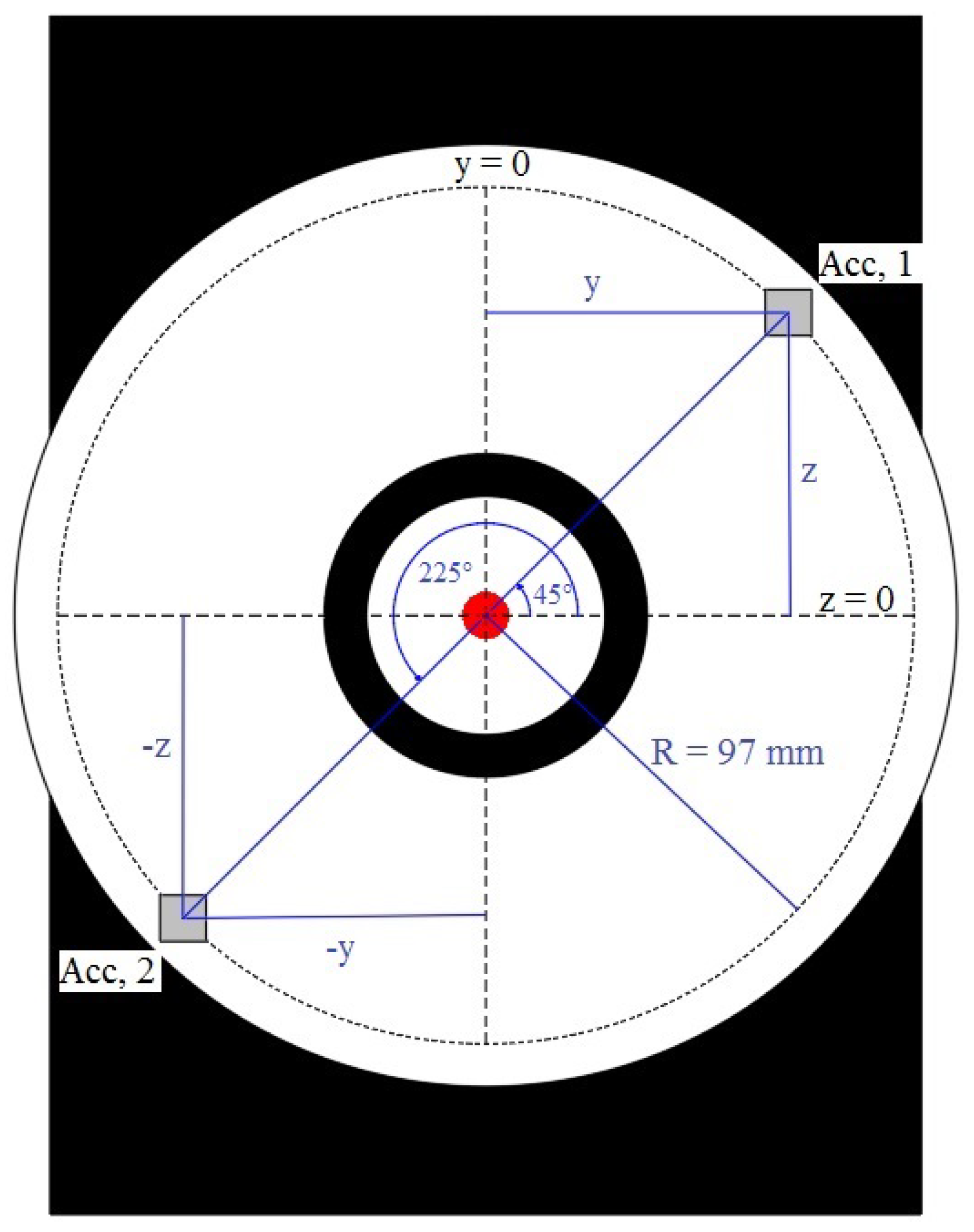
- 2 uni-axial accelerometers
- DAQ box for simultaneous data acquisition
- Portable computer
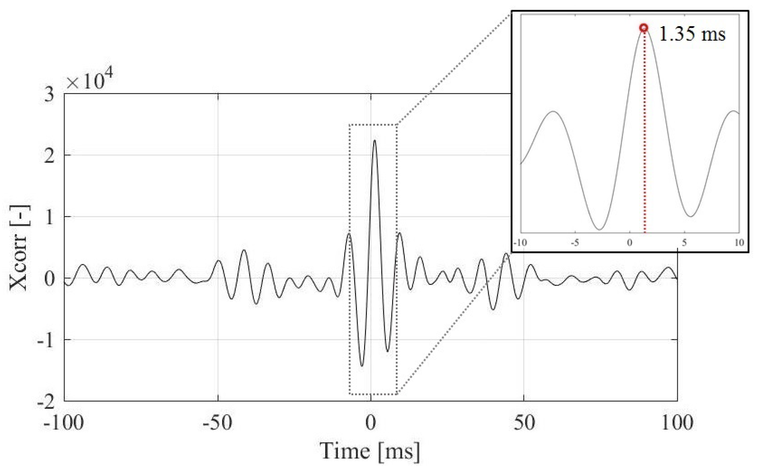
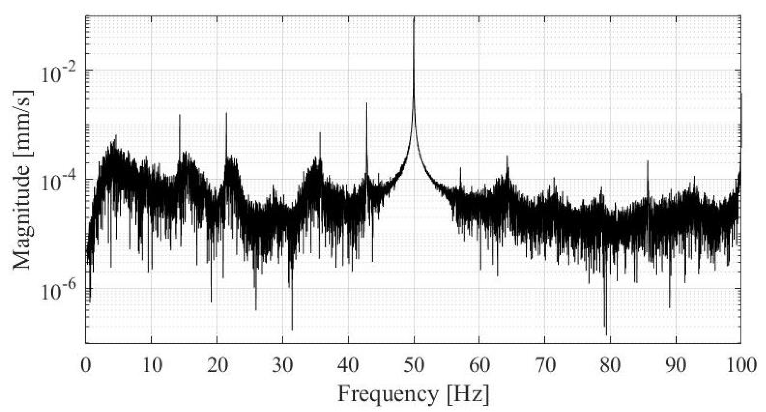
3.1. The Measurement Noise
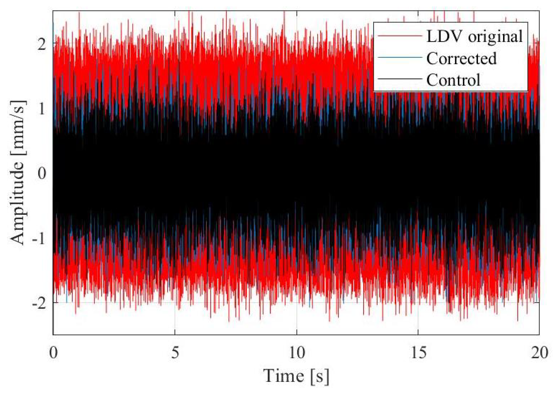
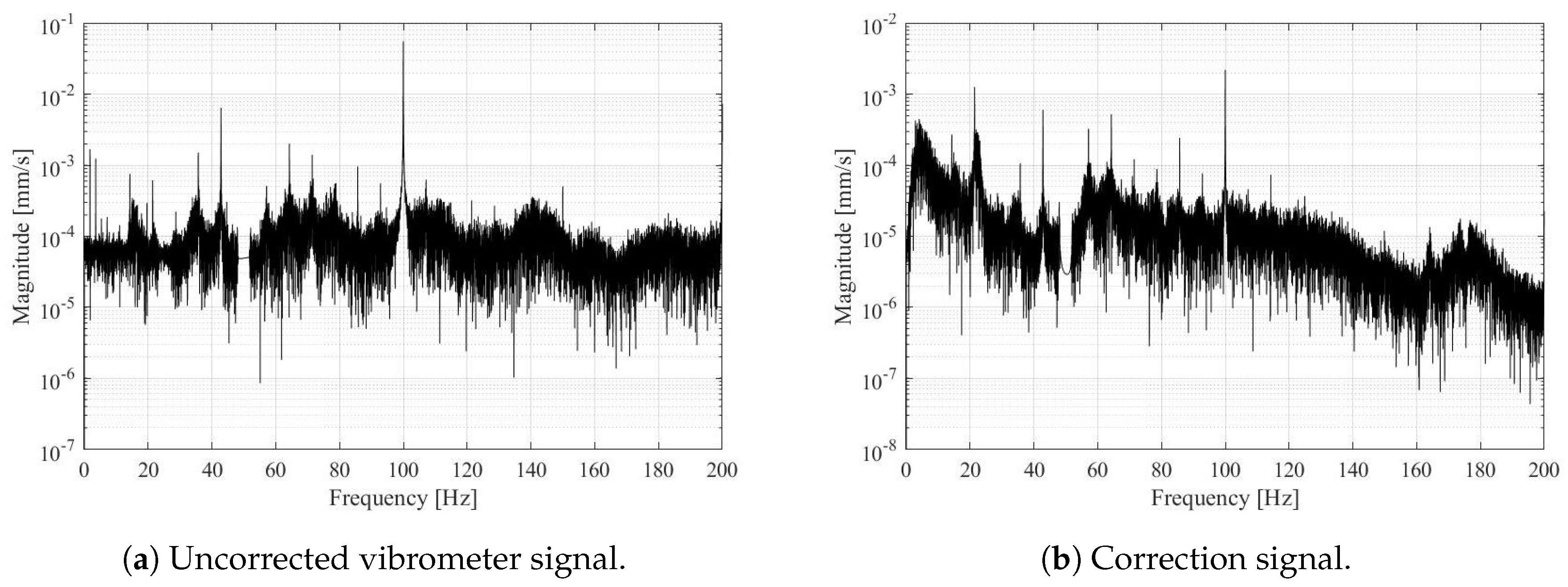
3.2. The Measurement of the Turbine during Regular Operation
4. Discussion and Conclusions
- we recommend to always use reflective tape (unless we have a clear reason why not to use it);
- whenever possible the standing point should be on a structurally different member than the surface under observation;
- the standing point should be on a structurally more rigid member than the point under observation;
- when measurements are done in strong sunlight the visor of the instrument must be shaded;
- methods to enhance signal-to-noise ratio should be applied together with an adequate anti-aliasing method with a proper measurement resolution.
Author Contributions
Funding
Acknowledgments
Conflicts of Interest
References
- Bernstone, C. Automated Performance Monitoring of Concrete Dams. Ph.D. Thesis, Lund University, Lund, Sweden, 2006. [Google Scholar]
- ICOLD Committee on Dam Ageing. Ageing of Dams and Appurtenant Works; Review and Recomendations. Bulletin 93; ICOLD-CIGB: Paris, France, 1994. [Google Scholar]
- ICOLD Technical Committee for Hydroelectric Energy. Dams for Hydroelectric Energy; Bulletin Preprint; ICOLD-CIGB: Paris, France, 2019. [Google Scholar]
- Trivedi, C.; Gandhi, B.K.; Cervantes, M.J.; Dahlhaug, O.G. Experimental investigations of a model Francis turbine during shutdown at synchronous speed. Renew. Energy 2015, 83, 828–836. [Google Scholar] [CrossRef]
- Deschênes, C.; Fraser, R.; Fau, J.P. New Trends in Turbine Modelling and New Ways of Partnership. In Proceedings of the International Conference on Hydraulic Efficiency Measurement-IGHEM, Toronto, ON, Canada, 17–19 July 2002; pp. 1–12. [Google Scholar]
- Trivedi, C.; Gandhi, B.; Cervantes, J.M. Effect of transients on Francis turbine runner life: A review. J. Hydraul. Res. 2013, 51, 121–132. [Google Scholar] [CrossRef]
- Urquiza, G.; García, J.C.; González, J.G.; Castro, L.; Rodríguez, J.A.; Basurto-Pensado, M.A. Failure analysis of a hydraulic Kaplan turbine shaft. Eng. Fail. Anal. 2014, 41, 108–117. [Google Scholar] [CrossRef]
- Goyal, R.; Gandhi, B.K. Review of hydrodynamics instabilities in Francis turbine during off-design and transient operations. Renew. Energy 2008, 116, 697–709. [Google Scholar] [CrossRef]
- Gasch, T.; Nässelqvist, M.; Hansson, H.; Malm, R.; Gustavsson, R.; Hassanzadeh, M. Cracking in the concrete foundation for hydropower generators. Part II Elforsk Rapp. 2013, 13, 68. [Google Scholar]
- Malm, R.; Hassanzadeh, M.; Gasch, T.; Eriksson, D.; Nordström, E. Cracking in the concrete foundation for hydropower generators Analyses of non-linear drying diffusion, thermal effects and mechanical loads. Elforsk Rapp. 2012, 13, 65. [Google Scholar]
- Lopez, F.; Restrepo Velez, L. Assessment and structural rehabilitation with post-tensioning and CFRP of a mass concrete structure subjected to dynamic loading. In Proceedings of the FIB Symposium Concrete Structures in Seismic Regions, Athens, Greece, l6–18 May 2003. [Google Scholar]
- Brownjohn, J.M.W.; de Stefano, A.; Xu, Y.-L.; Wenzel, H.; Aktan, A.E. Vibration-based monitoring of civil infrastructure: Challenges and successes. J. Civil Struct. Health Monit. 2011, 1, 79–95. [Google Scholar] [CrossRef]
- Hsieh, K.H.; Halling, M.W.; Barr, P.J. Overview of Vibrational Structural Health Monitoring with Representative Case Studies. J. Bridge Eng. 2006, 11, 707–715. [Google Scholar] [CrossRef]
- Cristalli, C.; Paone, N.; Rodríguez, R.M. Mechanical fault detection of electric motors by laser vibrometer and accelerometer measurements. Mech. Syst. Signal Process. 2006, 20, 1350–1361. [Google Scholar] [CrossRef]
- Yeh, Y.; Cummins, H.Z. Localized fluid flow measurements with an HeNe laser spectrometer. Appl. Phys. Lett. 1964, 4, 176–178. [Google Scholar] [CrossRef]
- Vanlanduit, S.; Dirckx, J. Editorial special issue on Laser Doppler vibrometry. Opt. Lasers Eng. 2017, 99, 1–2. [Google Scholar] [CrossRef]
- Gladiné, K.; Muyshondt, P.G.G.; Dirckx, J.J.J. Human middle-ear nonlinearity measurements using laser Doppler vibrometry. Opt. Lasers Eng. 2017, 99, 98–102. [Google Scholar] [CrossRef]
- Castellini, P.; Paone, N.; Tomasini, E.P. The Laser Doppler Vibrometer as an instrument for nonintrusive diagnostic of works of art: Application to fresco paintings. Opt. Lasers Eng. 1996, 25, 227–246. [Google Scholar] [CrossRef]
- Zucca, S.; Di Maio, D.; Ewins, D.J. Measuring the performance of underplatform dampers for turbine blades by rotating laser Doppler vibrometer. Mech. Syst. Signal Process. 2012, 32, 269–281. [Google Scholar] [CrossRef]
- Rothberg, S.J.; Allen, M.S.; Castellini, P.; Di Maio, D.; Dirckx, J.J.J.; Ewins, D.J.; Halkon, B.J.; Muyshondt, P.; Paone, N.; Ryan, T.; et al. An international review of laser Doppler vibrometry: Making light work of vibration measurement. Opt. Lasers Eng. 2017, 99, 11–22. [Google Scholar] [CrossRef]
- Strean, R.F.; Mitchell, L.D.; Barker, A.J. Global noise characteristics of a laser Doppler vibrometer 1. Theory. Opt. Lasers Eng. 1998, 30, 127–139. [Google Scholar] [CrossRef]
- Das, S.; Saha, P.; Patro, S.K. Vibration-based damage detection techniques used for health monitoring of structures: A review. J. Civil Struct. Health Monit. 2016, 6, 477–507. [Google Scholar] [CrossRef]
- Martin, P.; Rothberg, S.J. Laser vibrometry and the secret life of speckle patterns. In Proceedings of the Eighth International Conference on Vibration Measurements by Laser Techniques: Advances and Applications, Ancona, Italy, 18–20 June 2008. [Google Scholar] [CrossRef]
- Castellini, P.; Martarelli, M.; Tomasini, E.P. Laser Doppler Vibrometry: Development of advanced solutions answering to technology’s needs. Mech. Syst. Signal Process. 2006, 20, 1265–1285. [Google Scholar] [CrossRef]
- Agostinelli, G.; Cristalli, C.; Paone, N.; Serafini, S. Drop-out noise of laser vibrometers measuring on varnished steel surfaces of appliance cabinets for industrial diagnostics. In Proceedings of the AIP Conference Proceedings 9th International Conference on Vibration Measurements by Laser and Noncontact Techniques and Short Course, Ancona, Italy, 22–25 June 2010; pp. 298–312. [Google Scholar] [CrossRef]
- Agostinelli, G.; Paone, N. Uncertainty of diagnostic features measured by laser vibrometry: The case of optically non-cooperative surfaces. Opt. Lasers Eng. 2012, 50, 1804–1816. [Google Scholar] [CrossRef]
- Martin, P.; Rothberg, S.J. Pseudo-vibration sensitivities for commercial laser vibrometers. Mech. Syst. Signal Process. 2011, 25, 2753–2765. [Google Scholar] [CrossRef]
- Rothberg, S. Numerical simulation of speckle noise in laser vibrometry. Appl. Opt. 2006, 45, 4523–4533. [Google Scholar] [CrossRef] [PubMed]
- Martin, P.; Rothberg, S.J. Introducing speckle noise maps for Laser Vibrometry. Opt. Lasers Eng. 2009, 47, 431–442. [Google Scholar] [CrossRef]
- Halkon, B.J.; Rothberg, S.J. Taking laser Doppler vibrometry off the tripod: correction of measurements affected by instrument vibration. Opt. Lasers Eng. 2017, 91, 16–23. [Google Scholar] [CrossRef]
- DEWESoft. DEWESoft Measurement Innovation; User Manual; DEWESoft: Trbovlje, Slovenia, 2019. [Google Scholar]
- MATLAB R2018b. User’s Manual; The MathWorks Inc.: Massachusetts, MA, USA, 2018. [Google Scholar]
- Brincker, R.; Ventura, C. Introduction to Operational Modal Analysis; John Wiley & Sons, Ltd.: Chichester, UK, 2015; p. 376. [Google Scholar] [CrossRef]


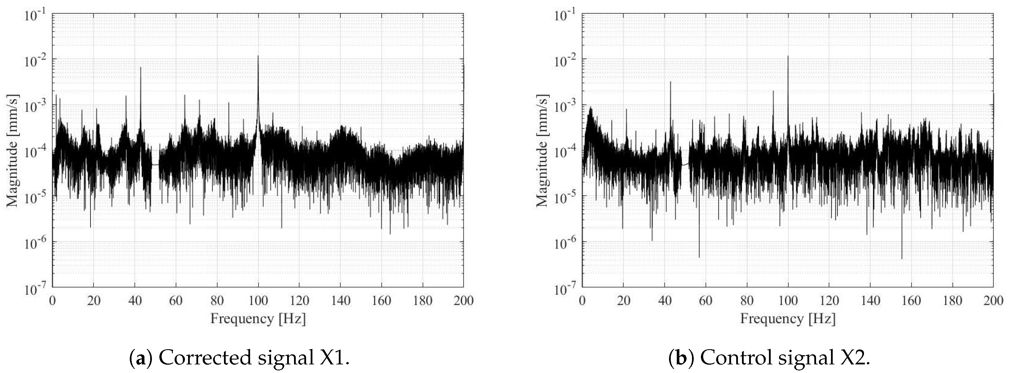
| Frequencies in the power spectrum [Hz] | 1.78, 3.56, 7.15, 21.43, 35.7, 42.85, 85.7, 100 |
© 2019 by the authors. Licensee MDPI, Basel, Switzerland. This article is an open access article distributed under the terms and conditions of the Creative Commons Attribution (CC BY) license (http://creativecommons.org/licenses/by/4.0/).
Share and Cite
Klun, M.; Zupan, D.; Lopatič, J.; Kryžanowski, A. On the Application of Laser Vibrometry to Perform Structural Health Monitoring in Non-Stationary Conditions of a Hydropower Dam. Sensors 2019, 19, 3811. https://doi.org/10.3390/s19173811
Klun M, Zupan D, Lopatič J, Kryžanowski A. On the Application of Laser Vibrometry to Perform Structural Health Monitoring in Non-Stationary Conditions of a Hydropower Dam. Sensors. 2019; 19(17):3811. https://doi.org/10.3390/s19173811
Chicago/Turabian StyleKlun, Mateja, Dejan Zupan, Jože Lopatič, and Andrej Kryžanowski. 2019. "On the Application of Laser Vibrometry to Perform Structural Health Monitoring in Non-Stationary Conditions of a Hydropower Dam" Sensors 19, no. 17: 3811. https://doi.org/10.3390/s19173811
APA StyleKlun, M., Zupan, D., Lopatič, J., & Kryžanowski, A. (2019). On the Application of Laser Vibrometry to Perform Structural Health Monitoring in Non-Stationary Conditions of a Hydropower Dam. Sensors, 19(17), 3811. https://doi.org/10.3390/s19173811