Guided Wave-Convolutional Neural Network Based Fatigue Crack Diagnosis of Aircraft Structures †


Abstract
:1. Introduction
2. GW-CNN Based Fatigue Crack Diagnosis Method
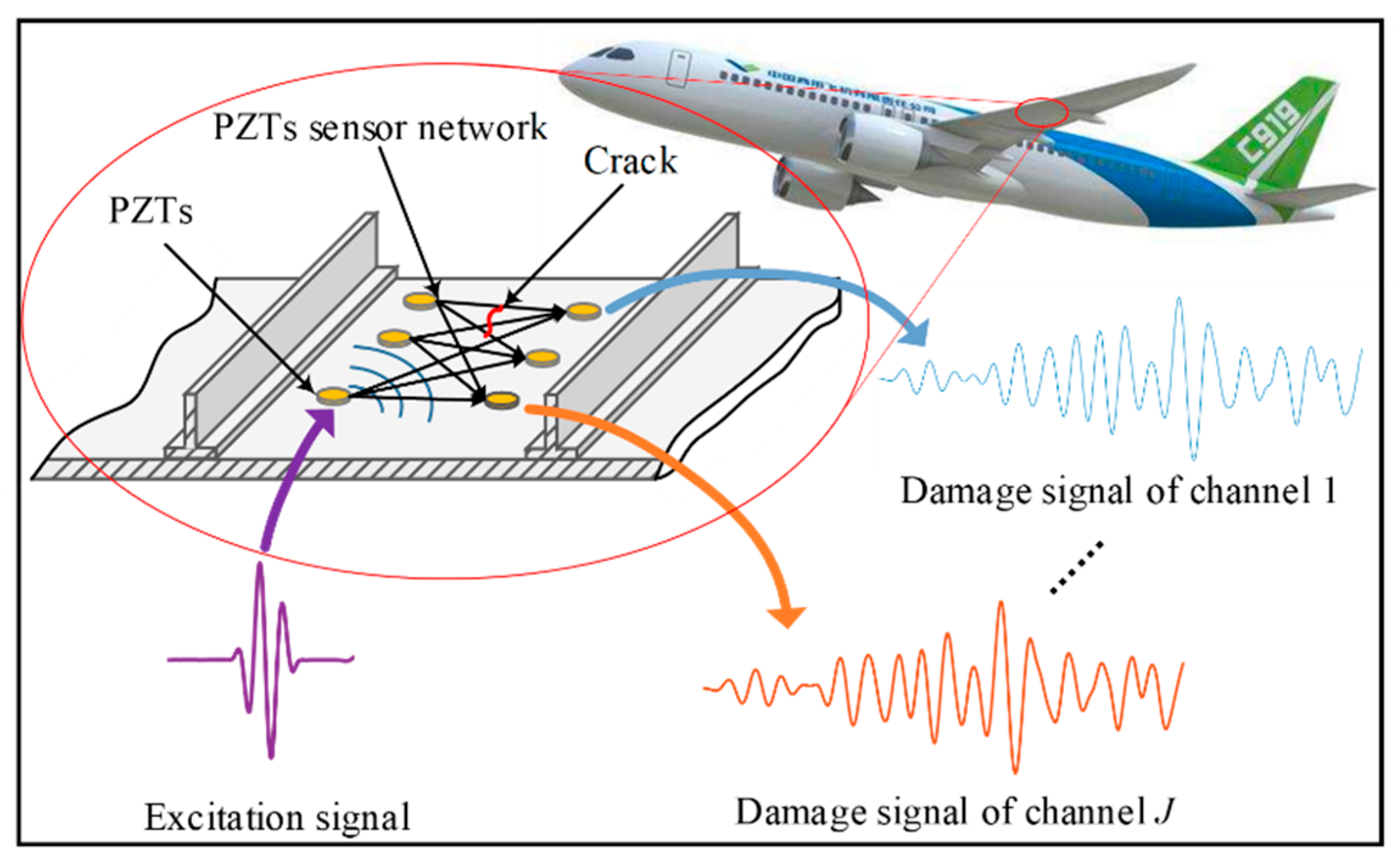
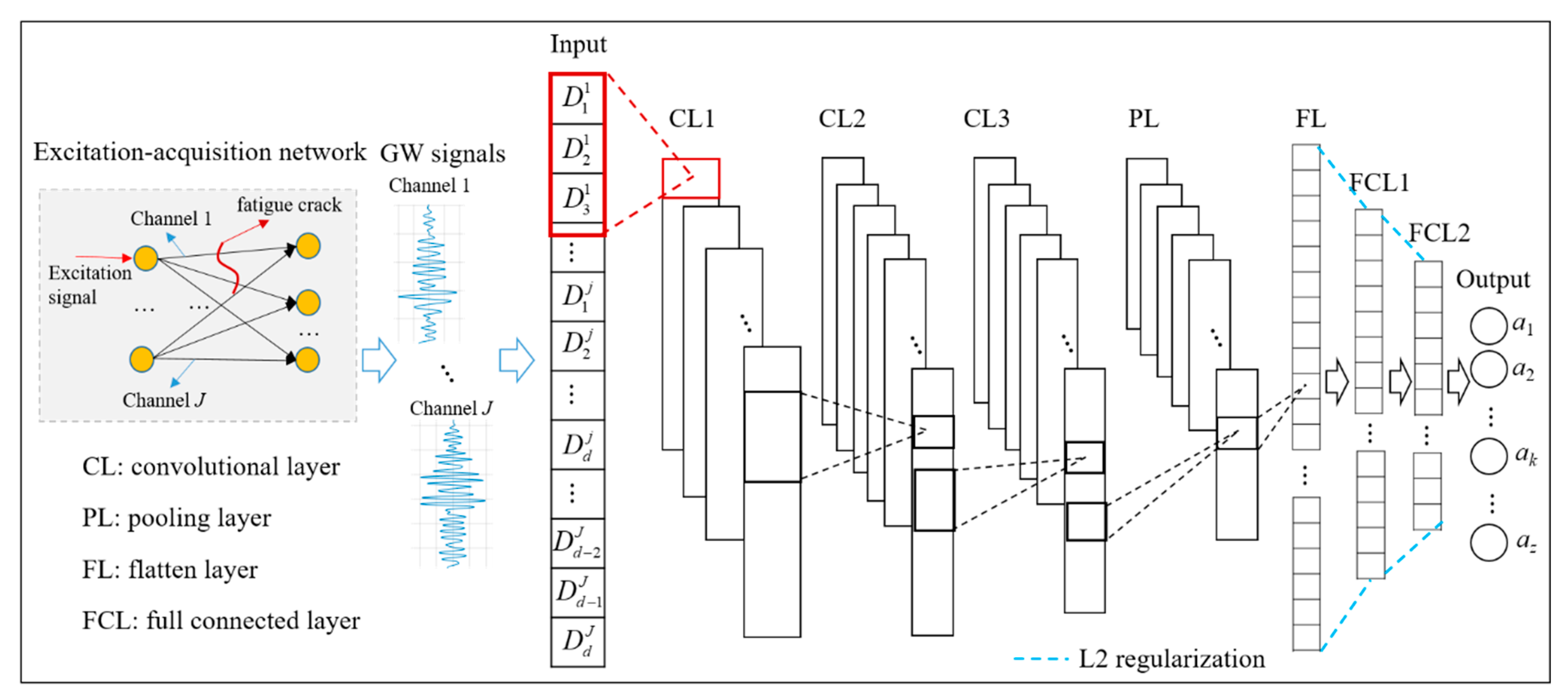
2.1. Multi-Channel and Multi-GW Features Extraction
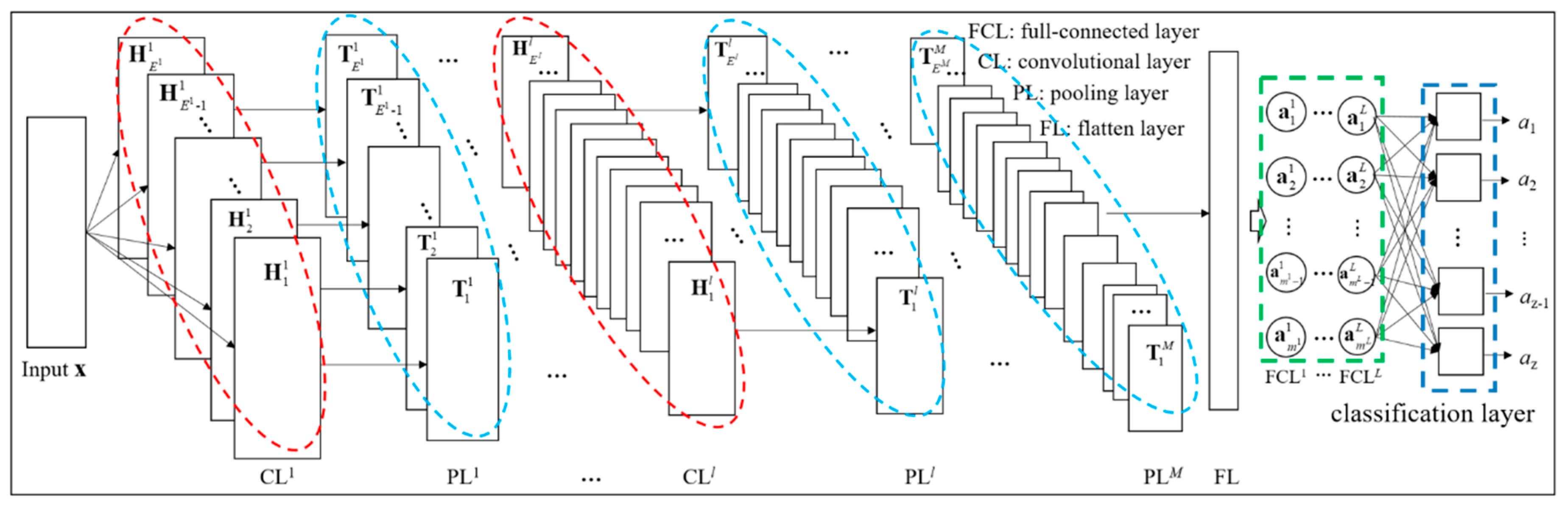
2.2. CNN Based Fatigue Crack Diagnosis
3. Experimental Verification and Analysis
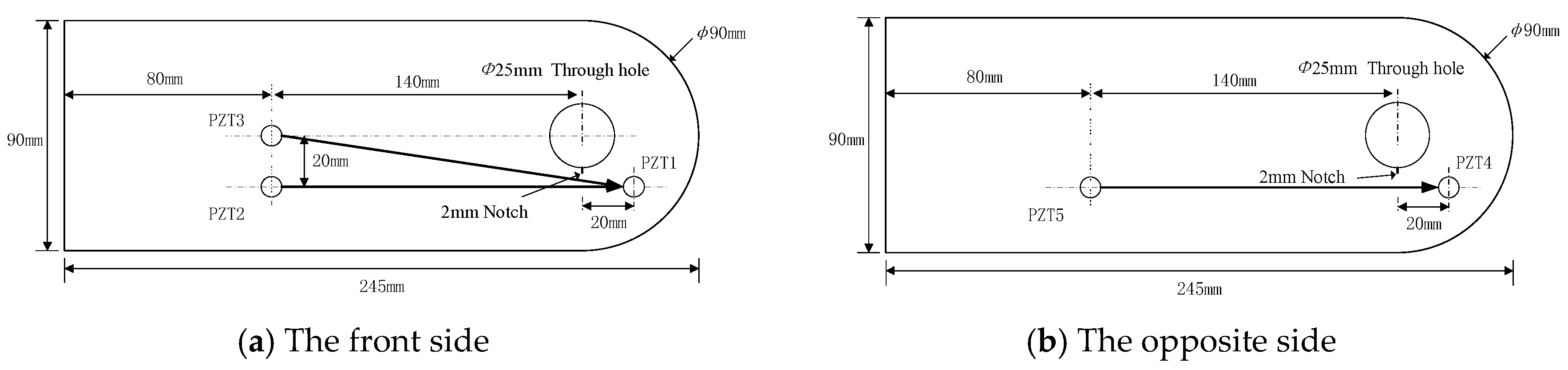
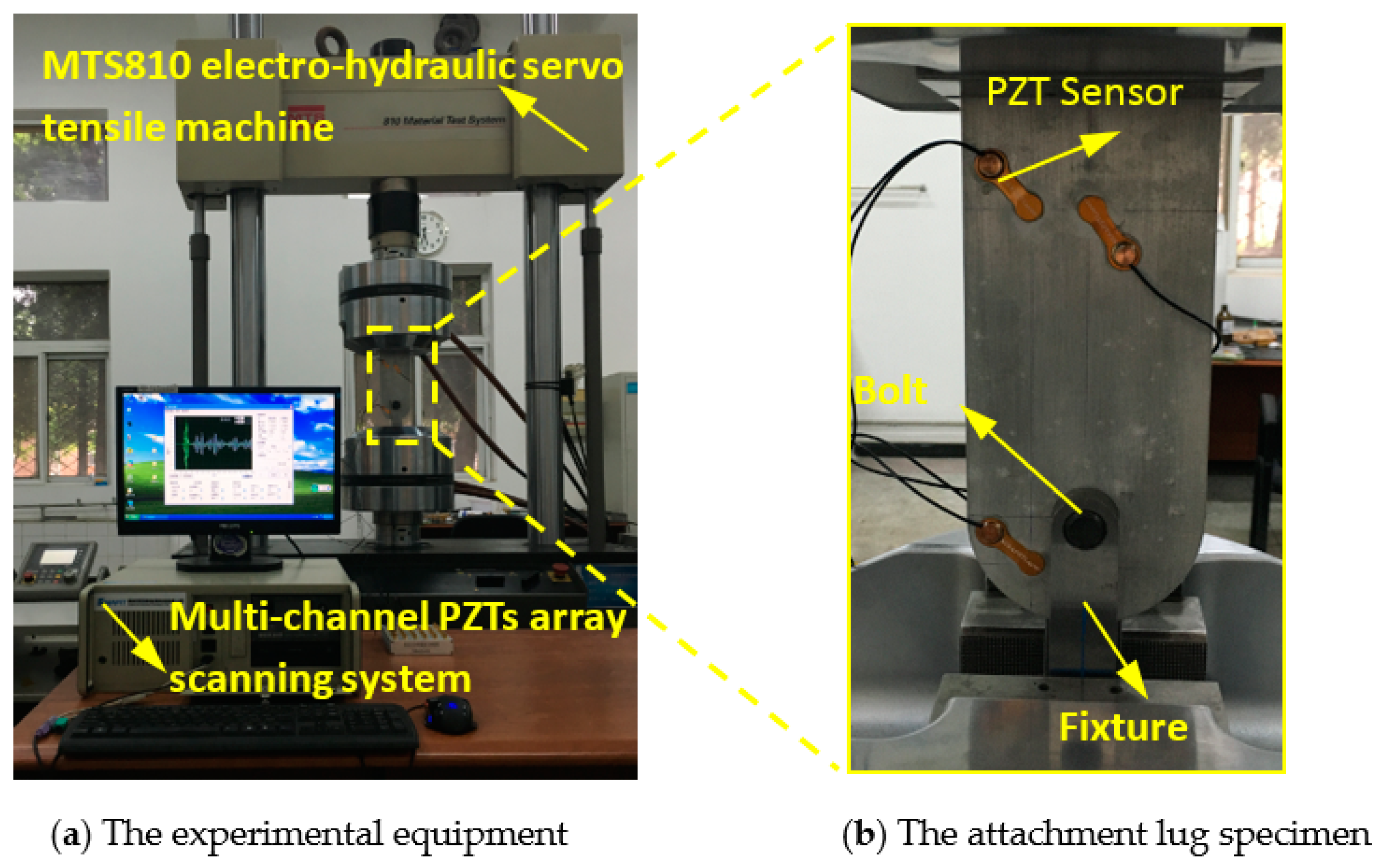
3.1. Fatigue Tests of Attachment Lug Specimens
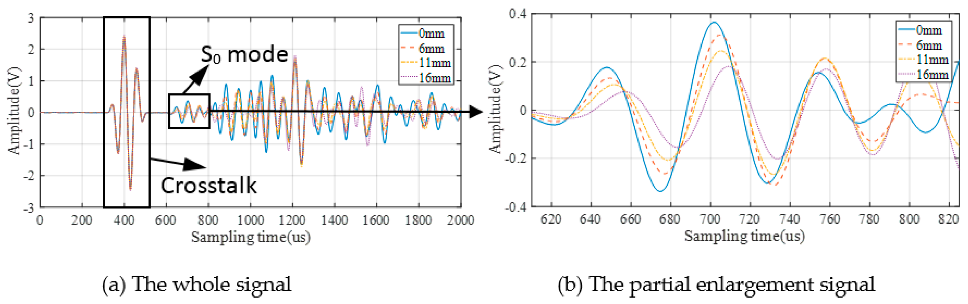
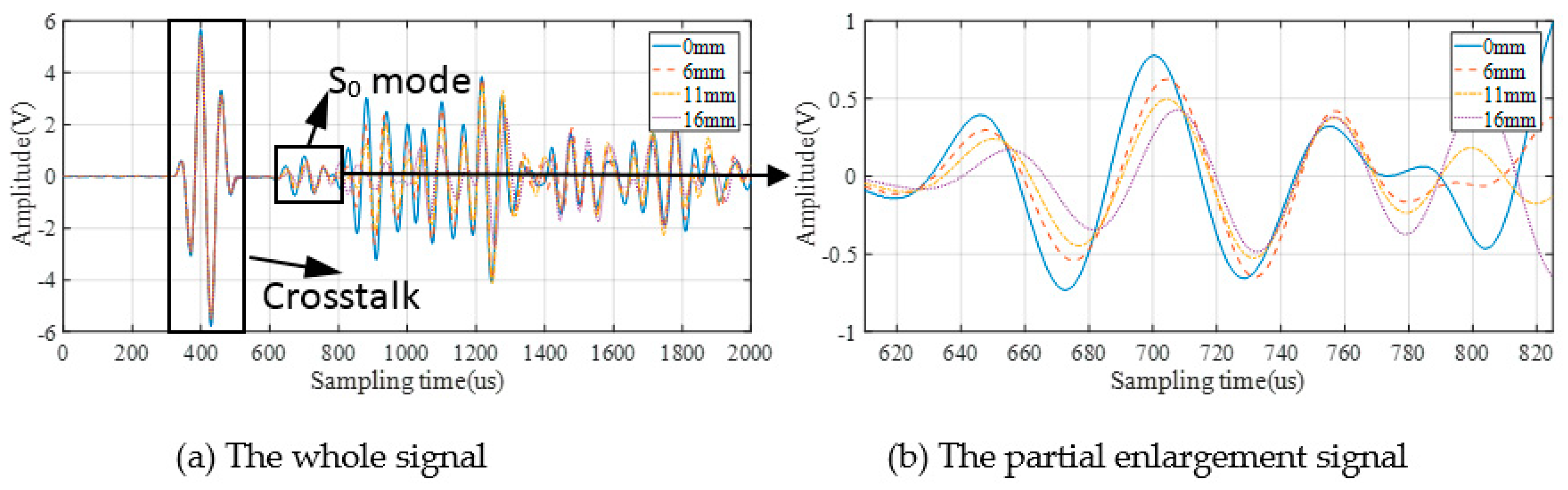
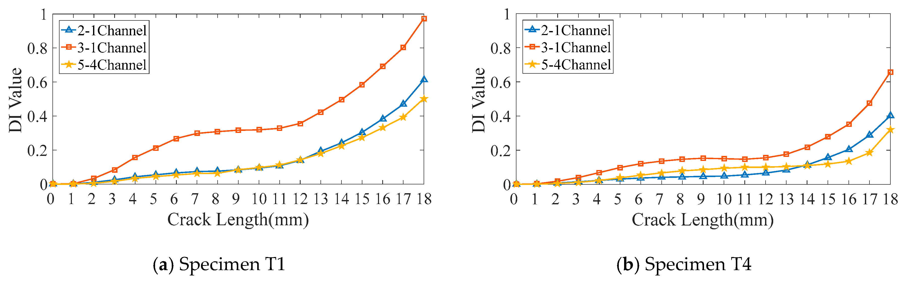
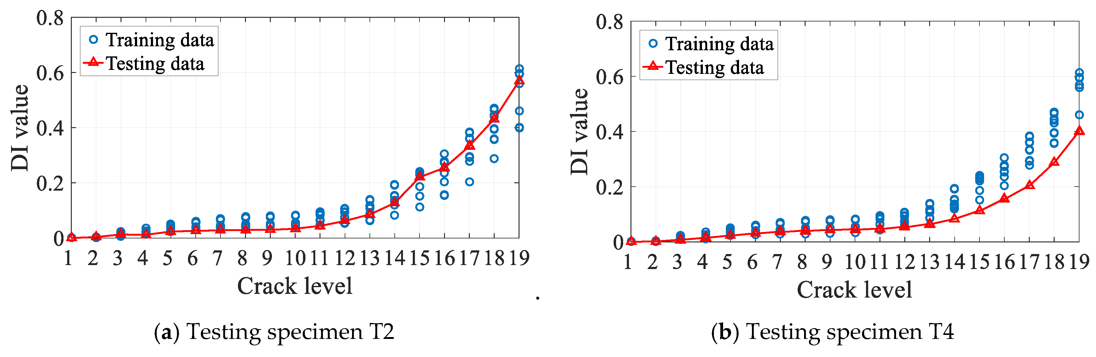
3.2. GW Monitoring and DIs Extraction
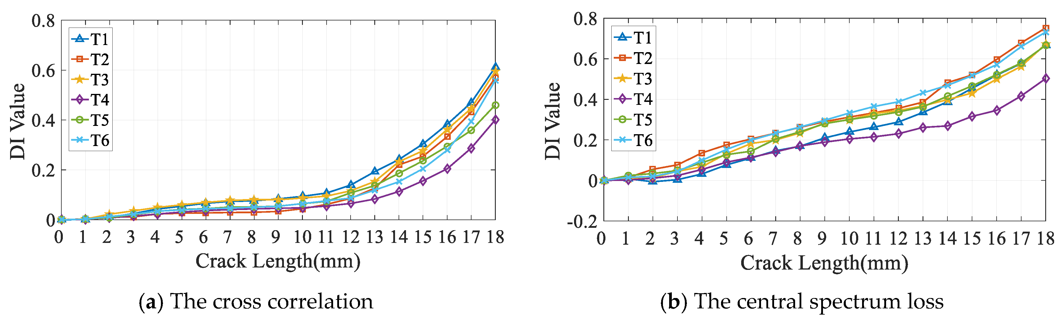
- The Cross correlation is a DI in the time domain, which is describe the degree of correlation between the normalized baseline signal and the monitoring signal;
- The Spatial phase difference is also a DI in the time domain that describes the size of the angle between the normalized baseline signal and the monitoring signal;
- The Spectrum loss is a DI in the frequency domain, which describes the difference value in spectrum between two signals;
- The Central spectrum loss is also a DI in the frequency domain, which measures the change of central spectrum between baseline and monitoring signal;
- The Differential curve energy is a DI that measured the variation of waveform curve of the difference of two signal;
- The Normalized Correlation Moment is a DI that based on local statistical features of the waveform; the energy and phase change of the signal has been taken into consideration;
- The differential signal energy is a DI that measured the variation of signal energy.
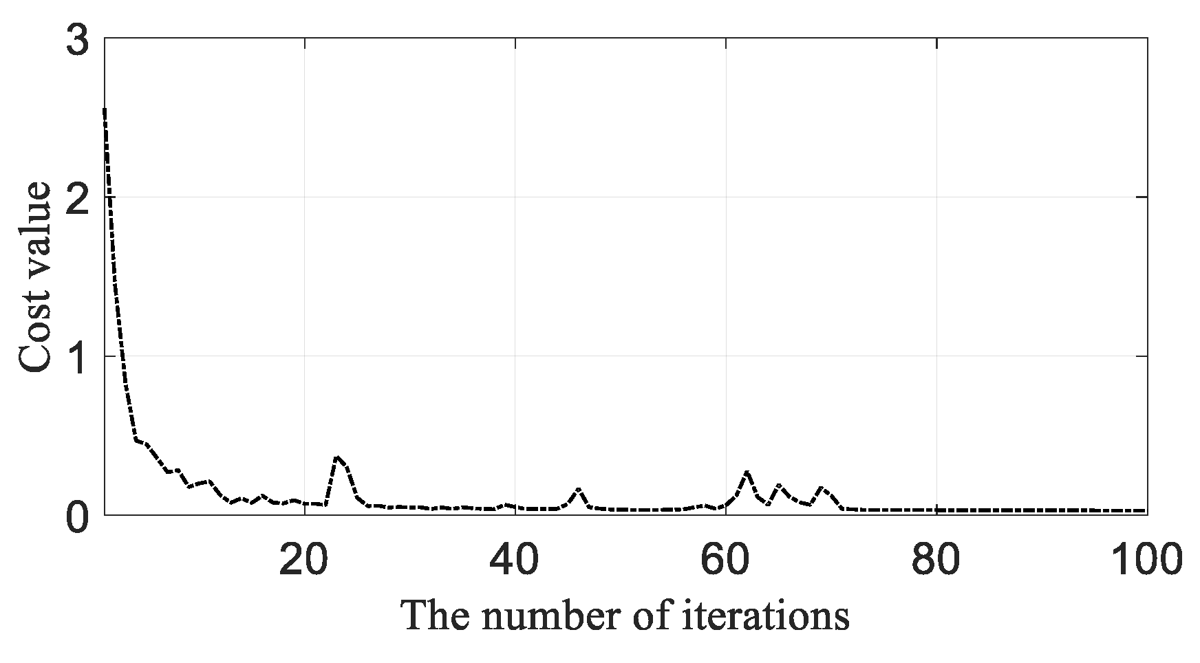
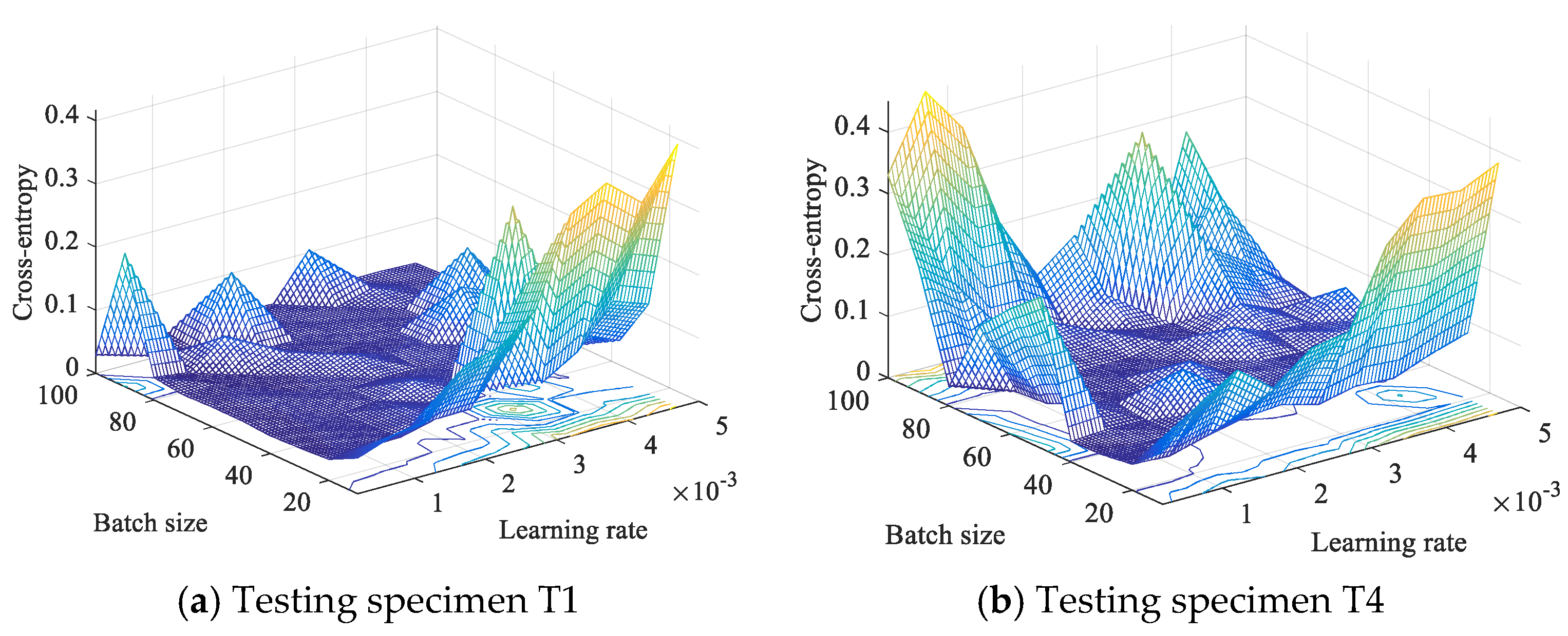
3.3. GW-CNN Based Diagnosis Training
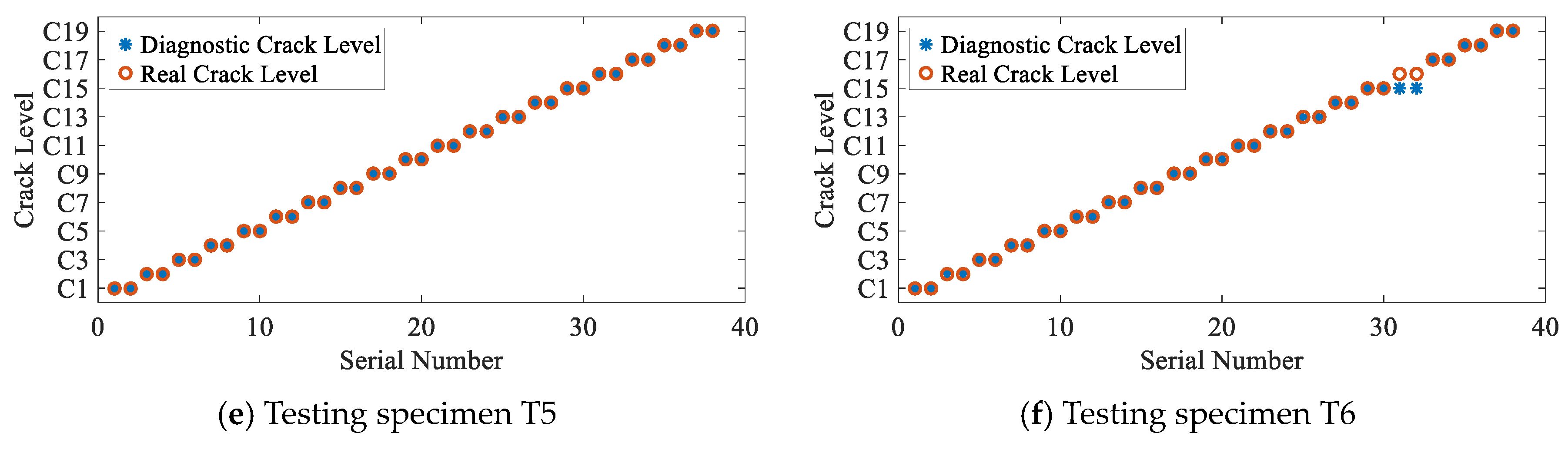
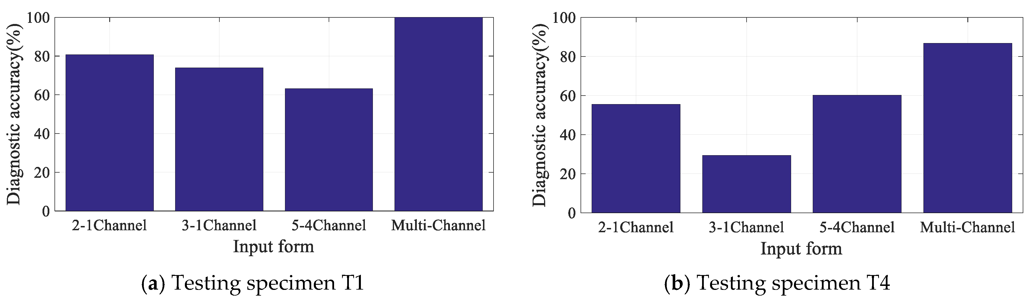
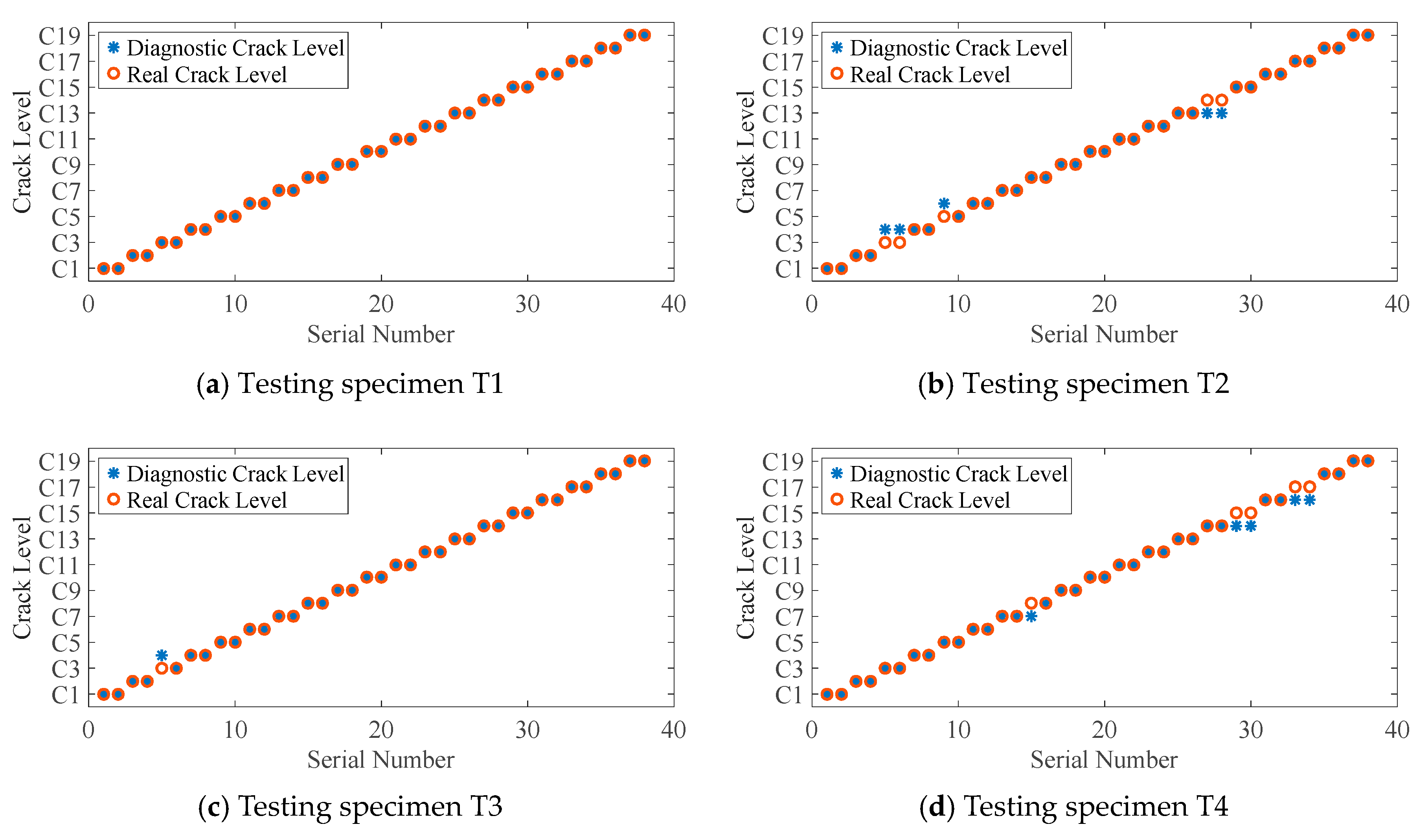
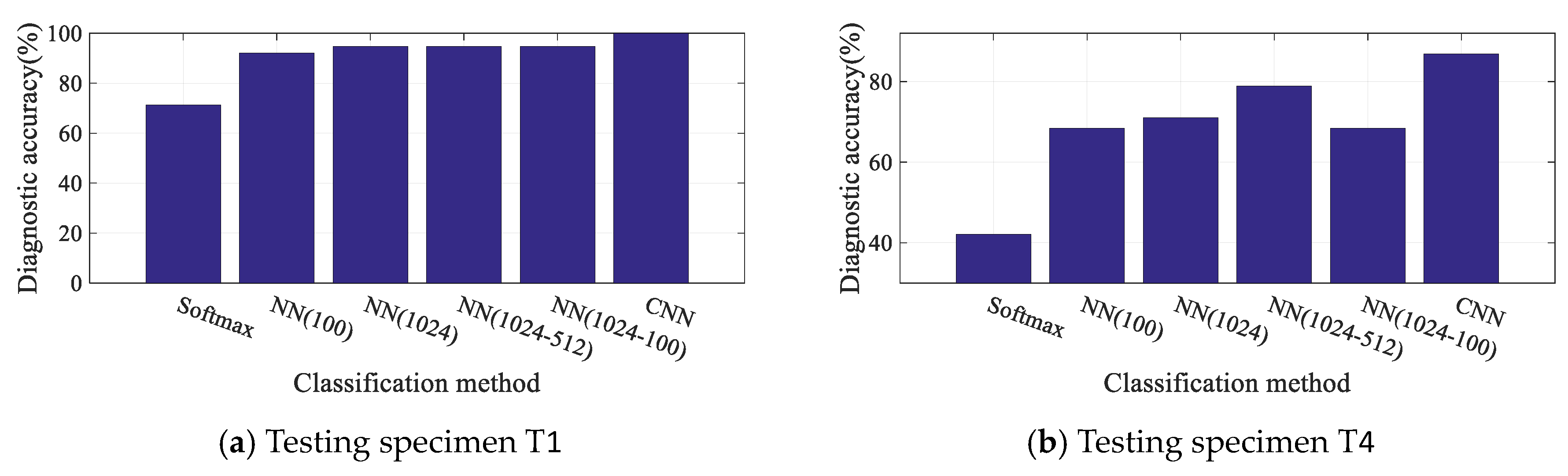
3.4. Diagnosis Results and Discussion
4. Conclusions
Author Contributions
Funding
Conflicts of Interest
References
- Xu, L.; Yuan, S.F.; Chen, J.; Bao, Q. Deep learning based fatigue crack diagnosis of aircraft structures. In Proceedings of the 7th Asia-Pacific Workshop on Structural Health Monitoring 2018, Hong Kong, China, 12–15 November 2018. [Google Scholar]
- Giurgiutiu, V.; Zagrai, A.; Bao, J.J. Piezoelectric Wafer Embedded Active Sensors for Aging Aircraft Structural Health Monitoring. Struct. Health Monit. 2002, 1, 41–61. [Google Scholar] [CrossRef]
- Duffour, P.; Morbidini, M.; Cawley, P. A study of the vibro-acoustic modulation technique for the detection of cracks in metals. J. Acoust. Soc. Am. 2006, 119, 1463. [Google Scholar] [CrossRef]
- Yuan, S.; Ren, Y.; Qiu, L.; Mei, H. A Multi-Response-Based Wireless Impact Monitoring Network for Aircraft Composite Structures. IEEE Trans. Ind. Electron. 2016, 63, 7712–7722. [Google Scholar] [CrossRef]
- Qiu, L.; Liu, B.; Yuan, S.; Su, Z.Q. Impact imaging of aircraft composite structure based on a model-independent spatial-wavenumber filter. Ultrasonics 2016, 64, 10–24. [Google Scholar] [CrossRef] [PubMed]
- Su, Z.Q.; Zhou, C.; Hong, M.; Cheng, L.; Wang, Q.; Qing, X. Acousto-ultrasonics-based fatigue damage characterization: Linear versus nonlinear signal features. Mech. Syst. Signal Process. 2014, 45, 225–239. [Google Scholar] [CrossRef]
- Michaels, J.; Michaels, T. Detection of structural damage from the local temporal coherence of diffuse ultrasonic signals. IEEE Trans. Ultrason. Ferroelectr. Freq. Control. 2005, 52, 1769–1782. [Google Scholar] [CrossRef] [PubMed]
- Lu, Y.; Michaels, J. Feature Extraction and Sensor Fusion for Ultrasonic Structural Health Monitoring Under Changing Environmental Conditions. IEEE Sens. J. 2009, 9, 1462–1471. [Google Scholar]
- Torkamani, S.; Roy, S.; Barkey, M.E.; Sazonov, E.; Burkett, S.; Kotru, S. A novel damage index for damage identification using guided waves with application in laminated composites. Smart Mater. Struct. 2014, 23, 95015. [Google Scholar] [CrossRef]
- Mitra, M.; Gopalakrishnan, S. Guided wave based structural health monitoring: A review. Smart Mater. Struct. 2016, 25, 53001. [Google Scholar] [CrossRef]
- Mei, H.; Yuan, S.; Qiu, L.; Zhang, J. Damage evaluation by a guided wave-hidden Markov model based method. Smart Mater. Struct. 2016, 25, 25021. [Google Scholar] [CrossRef]
- Qiu, L.; Yuan, S.; Chang, F.; Bao, Q.; Mei, H. On-line updating Gaussian mixture model for aircraft wing spar damage evaluation under time-varying boundary condition. Smart Mater. Struct. 2014, 23, 125001. [Google Scholar] [CrossRef]
- Qiu, L.; Yuan, S.; Boller, C. An adaptive guided wave-Gaussian mixture model for damage monitoring under time-varying conditions: Validation in a full-scale aircraft fatigue test. Struct. Health Monit. 2017, 16, 501–517. [Google Scholar] [CrossRef]
- Gu, J.; Gul, M.; Wu, X. Damage detection under varying temperature using artificial neural networks. Struct. Control. Health Monit. 2017, 24, e1998. [Google Scholar] [CrossRef]
- Gui, G.; Pan, H.; Lin, Z.; Li, Y.; Yuan, Z. Data-driven support vector machine with optimization techniques for structural health monitoring and damage detection. KSCE J. Civ. Eng. 2017, 21, 523–534. [Google Scholar] [CrossRef]
- Taha, M.R.; Lucero, J. Damage identification for structural health monitoring using fuzzy pattern recognition. Eng. Struct. 2005, 27, 1774–1783. [Google Scholar] [CrossRef]
- LeCun, Y.; Bengio, Y.; Hinton, G. Deep learning. Nature 2015, 521, 436–444. [Google Scholar] [CrossRef] [PubMed]
- Hinton, G.; Deng, L.; Yu, D.; Dahl, G.; Mohamed, A.R.; Jaitly, N.; Sainath, T. Deep neural networks for acoustic modeling in speech recognition. IEEE Signal Process. Mag. 2012, 29, 82–97. [Google Scholar] [CrossRef]
- Esteva, A.; Kuprel, B.; Novoa, R.A.; Ko, J.; Swetter, S.M.; Blau, H.M.; Thrun, S. Dermatologist-level classification of skin cancer with deep neural networks. Nature 2017, 542, 115–118. [Google Scholar] [CrossRef]
- Goodfellow, I.; Bengio, Y.; Courville, A. Deep Learning; MIT Press: Cambridge, MA, USA, 2016. [Google Scholar]
- Shao, S.; Sun, W.; Zhao, R.; Yan, R.; Chen, X. Convolutional Discriminative Feature Learning for Induction Motor Fault Diagnosis. IEEE Trans. Ind. Inform. 2017, 13, 1350–1359. [Google Scholar]
- Guo, X.; Chen, L.; Shen, C. Hierarchical adaptive deep convolution neural network and its application to bearing fault diagnosis. Measurement 2016, 93, 490–502. [Google Scholar] [CrossRef]
- Grus, J. Data Science from Scratch: First Principles with Python; O’Reilly Media, Inc.: Sebastopol, CA, USA, 2015; pp. 99–100. [Google Scholar]
- Liao, B.; Xu, J.; Lv, J.; Zhou, S. An Image Retrieval Method for Binary Images Based on DBN and Softmax Classifier. IETE Tech. Rev. 2015, 32, 1–10. [Google Scholar] [CrossRef]
- Smith, L.N.; Topin, N. Deep Convolutional Neural Network Design Patterns 2016. arXiv 2016, arXiv:1611.00847. [Google Scholar]
- Nielsen, M. Neural Networks and Deep Learning; Determination Press: San Francisco, CA, USA, 2015. [Google Scholar]
- Glorot, X.; Bengio, Y. Understanding the difficulty of training deep feedforward neural networks. In Proceedings of the Thirteenth International Conference on Artificial Intelligence and Statistics, Sardinia, Italy, 13–15 May 2010; pp. 249–256. [Google Scholar]
- Kingma, D.; Ba, J. Adam: A method for stochastic optimization. arXiv 2014, arXiv:1412.6980. [Google Scholar]
- Qiu, L.; Yuan, S. On development of a multi-channel PZT array scanning system and its evaluating application on UAV wing box. Sens. Actuators A Phys. 2009, 151, 220–230. [Google Scholar] [CrossRef]


| Damage IndexDI | Extraction Algorithm |
|---|---|
| Cross correlation [6] | |
| Spatial phase difference | |
| Spectrum loss | |
| Central spectrum loss | |
| Differential curve energy [7] | |
| Normalized Correlation Moment [8] | |
| Differential signal energy |
| Crack Size | C1 | C2 | C3 | C4 | C5 | C6 | C7 | C8 | C9 | C10 |
| Crack length (mm) | 0 | 1 | 2 | 3 | 4 | 5 | 6 | 7 | 8 | 9 |
| Crack size | C11 | C12 | C13 | C14 | C15 | C16 | C17 | C18 | C19 | |
| Crack length (mm) | 10 | 11 | 12 | 13 | 14 | 15 | 16 | 17 | 18 |
| Testing Specimen | T1 | T2 | T3 | T4 | T5 | T6 |
|---|---|---|---|---|---|---|
| Training specimens | T2–T6 | T1, T3–T6 | T1–T2, T4–T6 | T1–T3, T5–T6 | T1–T4, T6 | T1–T5 |
| Testing Specimen | T1 | T2 | T3 | T4 | T5 | T6 |
|---|---|---|---|---|---|---|
| Accuracy | 100% | 86.84% | 97.37% | 86.84% | 100% | 94.74% |
| Crack Size | Input Samples | Output Features | ||||
|---|---|---|---|---|---|---|
| C7 | 2.0159 | 0.2142 | 1.8326 | 0.0002 | 0.0016 | 0.0011 |
| C18 | 0.0204 | 0.0253 | 0.0137 | 0.0002 | 0.0011 | 0.0015 |
| Classification Method | Softmax | NN (100) | NN (1024) | NN (1024-512) | NN (512-100) | CNN |
|---|---|---|---|---|---|---|
| T1 | 89 s | 59 s | 33 s | 89 s | 50 s | 14 s |
| T4 | 35 s | 117 s | 117 s | 86 s | 57 s | 9 s |
© 2019 by the authors. Licensee MDPI, Basel, Switzerland. This article is an open access article distributed under the terms and conditions of the Creative Commons Attribution (CC BY) license (http://creativecommons.org/licenses/by/4.0/).
Share and Cite
Xu, L.; Yuan, S.; Chen, J.; Ren, Y. Guided Wave-Convolutional Neural Network Based Fatigue Crack Diagnosis of Aircraft Structures. Sensors 2019, 19, 3567. https://doi.org/10.3390/s19163567
Xu L, Yuan S, Chen J, Ren Y. Guided Wave-Convolutional Neural Network Based Fatigue Crack Diagnosis of Aircraft Structures. Sensors. 2019; 19(16):3567. https://doi.org/10.3390/s19163567
Chicago/Turabian StyleXu, Liang, Shenfang Yuan, Jian Chen, and Yuanqiang Ren. 2019. "Guided Wave-Convolutional Neural Network Based Fatigue Crack Diagnosis of Aircraft Structures" Sensors 19, no. 16: 3567. https://doi.org/10.3390/s19163567
APA StyleXu, L., Yuan, S., Chen, J., & Ren, Y. (2019). Guided Wave-Convolutional Neural Network Based Fatigue Crack Diagnosis of Aircraft Structures. Sensors, 19(16), 3567. https://doi.org/10.3390/s19163567