Measurement Method Based on Multispectral Three-Dimensional Imaging for the Chlorophyll Contents of Greenhouse Tomato Plants


Abstract
1. Introduction
2. Materials and Methods
2.1. Sample Cultivation
2.2. Instrument and Chlorophyll Content Measurement
2.3. Multispectral 3D Point Cloud Modeling
2.3.1. Spectral Reflectance Registration
2.3.2. 3D Reconstruction of Multiview RGB-D Images
2.4. Data Processing
3. Results and Analysis
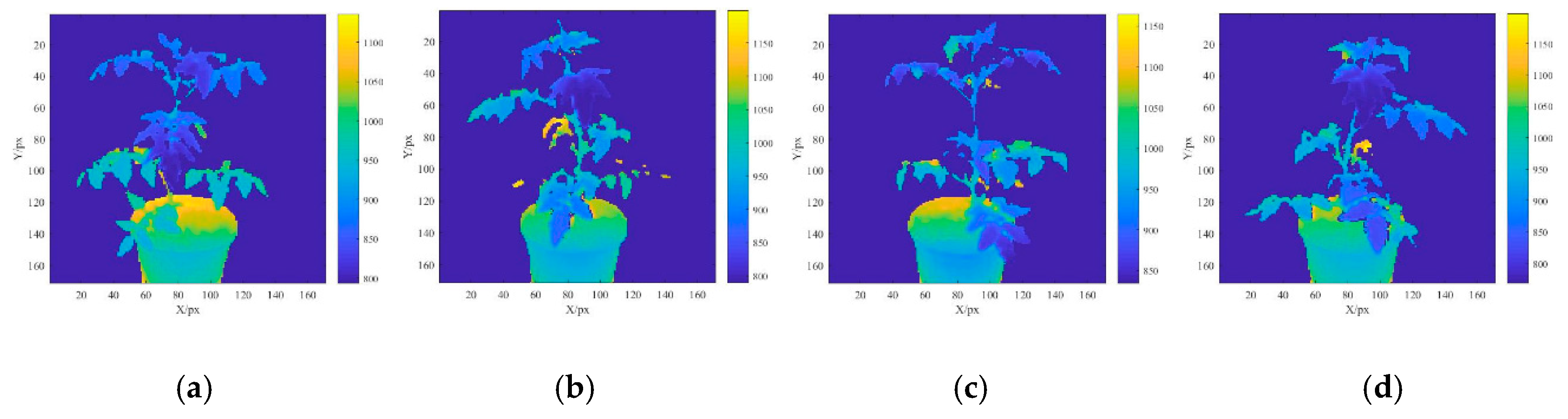
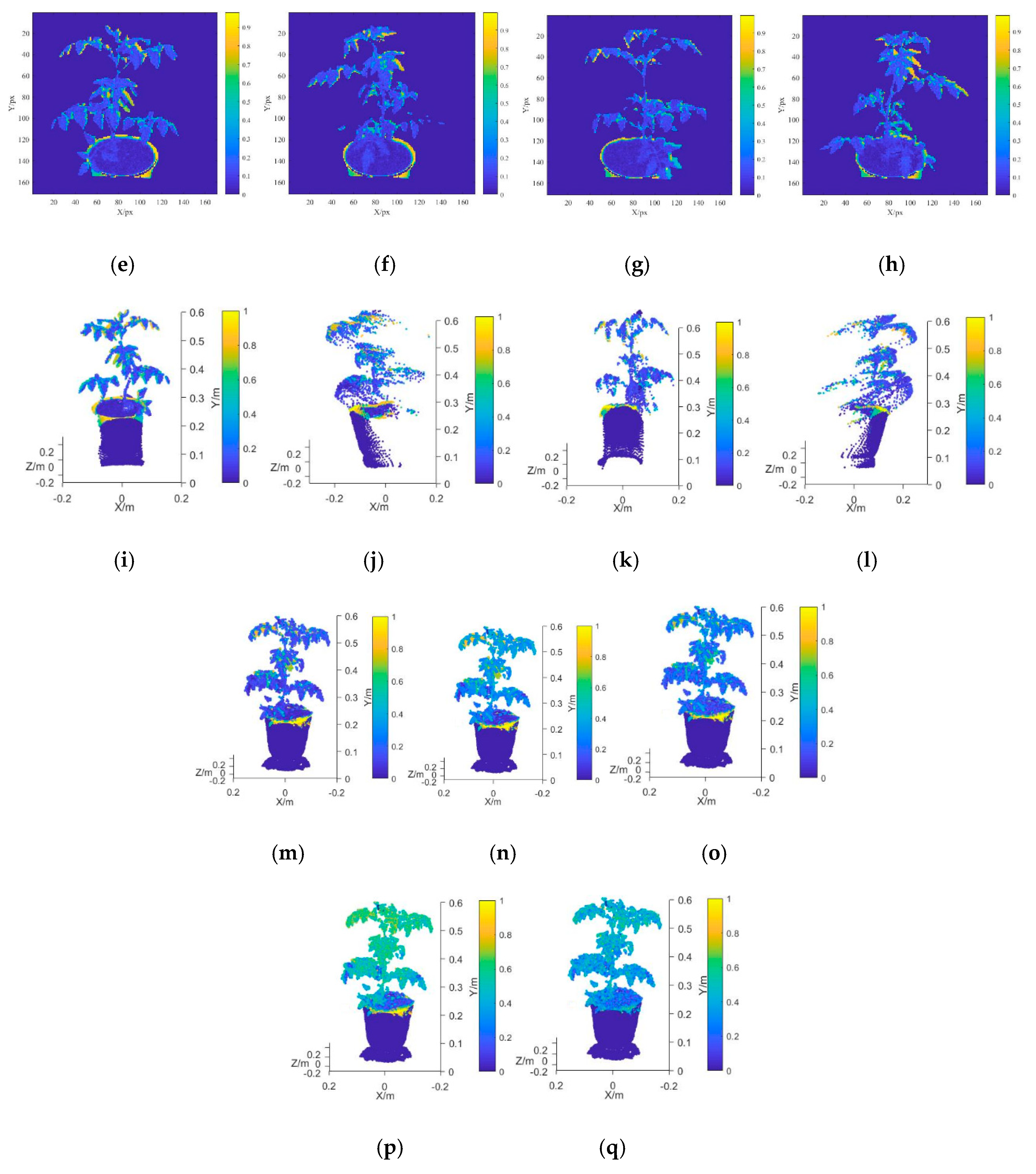
3.1. Multispectral 3D Point Cloud Modeling
3.2. Spectral Reflectance Variability Analysis
3.3. Plant Chlorophyll Measurement Model and Analysis
4. Conclusions
Author Contributions
Funding
Acknowledgments
Conflicts of Interest
References
- Padilla, F.M.; Gallardo, M.; Pena-Fleitas, M.T.; de Souza, R.; Thompson, R.B. Proximal optical sensors for nitrogen management of vegetable crops: A review. Sensors 2018, 18, 2083. [Google Scholar] [CrossRef]
- Yang, Z.; Hu, J.; Duan, T.; Wang, S.; Wu, J.; Su, W.; Zhang, Y. Research progress of nondestructive diagnostic technique of chlorophyll in plants. Chin. Agric. Sci. Bull. 2019, 35, 139–144. [Google Scholar]
- Lin, F.F.; Qiu, L.F.; Deng, J.S.; Shi, Y.Y.; Chen, L.S.; Wang, K. Investigation of SPAD meter-based indices for estimating rice nitrogen status. Comput. Electron. Agric. 2010, 71, S60–S65. [Google Scholar] [CrossRef]
- Padilla, F.M.; Peña-Fleitas, M.T.; Gallardo, M.; Giménez, C.; Thompson, R.B. Derivation of sufficiency values of a chlorophyll meter to estimate cucumber nitrogen status and yield. Comput. Electron. Agric. 2017, 141, 54–64. [Google Scholar] [CrossRef]
- Ghasemi, M.; Arzani, K.; Yadollahi, A.; Ghasemi, S.; Khorrami, S.S. Estimate of leaf chlorophyll and nitrogen content in Asian pear (Pyrus serotina Rehd.) by CCM-200. Not. Sci. Biol. 2011, 3, 91–94. [Google Scholar] [CrossRef][Green Version]
- He, Y.; Peng, J.; Liu, F.; Zhang, C.; Kong, W. Critical review of fast detection of crop nutrient and physiological information with spectral and imaging technology. Trans. Chin. Soc. Agric. Eng. 2015, 31, 174–189. [Google Scholar]
- He, Y.; Zhao, C.; Wu, D. Fast detection technique and sensor instruments for crop-environment information: A review. Sci. China Ser. F Inf. Sci. 2010, 40, 1–20. [Google Scholar]
- Wang, X.; Huang, J. Principles and Techniques of Plant Physiological Biochemical Experiment; Higher Education Press: Beijing, China, 2006; pp. 134–136. [Google Scholar]
- Perez-Patricio, M.; Camas-Anzueto, J.L.; Sanchez-Alegria, A.; Aguilar-Gonzalez, A.; Gutierrez-Miceli, F.; Escobar-Gomez, E.; Voisin, Y.; Rios-Rojas, C.; Grajales-Coutino, R. Optical method for estimating the chlorophyll contents in plant leaves. Sensors 2018, 18, 650. [Google Scholar] [CrossRef]
- Jörg, P.; Pablo, R.; Hu, Y.; Sebastian, K.; Gero, B.; Bodo, M.; Urs, S. Use of a digital camera as alternative method for non-destructive detection of the leaf chlorophyll content and the nitrogen nutrition status in wheat. Comput. Electron. Agric. 2017, 140, 25–33. [Google Scholar] [CrossRef]
- Dario, C.P.; Maria, C.; Bernardo, P.; Antonio, F.L.; Giovanni, A. Contactless and non-destructive chlorophyll content prediction by random forest regression: A case study on fresh-cut rocket leaves. Comput. Electron. Agric. 2017, 140, 303–310. [Google Scholar] [CrossRef]
- Liang, Y.; Daisuke, U.; Liao, K.-L.; Hedrick, T.L.; Gao, Y.; Jones, A.M. A nondestructive method to estimate the chlorophyll content of Arabidopsis seedlings. Plant Methods 2017, 13, 26. [Google Scholar] [CrossRef]
- Wang, Y.; Wang, D.; Shi, P.; Kenji, O. Estimating rice chlorophyll content and leaf nitrogen concentration with a digital still color camera under natural light. Plant Methods 2014, 10, 36. [Google Scholar] [CrossRef]
- Avinash, A.; Snehasish, D.G. Assessment of spinach seedling health status and chlorophyll content by multivariate data analysis and multiple linear regression of leaf image features. Comput. Electron. Agric. 2018, 152, 281–289. [Google Scholar] [CrossRef]
- Rei, S.; Tomohito, S.; Hideki, H. Using spectral reflectance to estimate leaf chlorophyll content of tea with shading treatments. Biosyst. Eng. 2018, 175, 168–182. [Google Scholar] [CrossRef]
- Yu, K.-Q.; Zhao, Y.-R.; Zhu, F.-L.; Li, X.-L.; He, Y. Mapping of chlorophyll and SPAD distribution in pepper leaves during leaf senescence using visible and near-infrared hyperspectral imaging. Trans. ASABE 2016, 59, 13–24. [Google Scholar] [CrossRef]
- Liu, B.; Yue, Y.M.; Li, R.; Shen, W.J.; Wang, K.L. Plant leaf chlorophyll content retrieval based on a field imaging spectroscopy system. Sensors 2014, 14, 19910–19925. [Google Scholar] [CrossRef]
- Zhang, J.; Han, W.; Huang, L.; Zhang, Z.; Ma, Y.; Hu, Y. Leaf chlorophyll content estimation of winter wheat based on visible and near-infrared sensors. Sensors 2016, 16, 437. [Google Scholar] [CrossRef]
- Qin, C.; Huang, J.; Wang, H.; Sun, H.; Zhang, Y.; Li, Y. Polarized hyperspectral characteristics and the ralationship with chlorophyll content of smooth leaves. J. Meteorol. Sci. 2019, 39, 421–426. [Google Scholar]
- Kuckenberg, J.; Tartachnyk, I.; Noga, G. Detection and differentiation of nitrogen-deficiency, powdery mildew and leaf rust at wheat leaf and canopy level by laser-induced chlorophyll fluorescence. Biosyst. Eng. 2009, 103, 121–128. [Google Scholar] [CrossRef]
- Thapa, S.; Zhu, F.; Walia, H.; Yu, H.; Ge, Y. A novel LiDAR-based instrument for high-throughput, 3D measurement of morphological traits Maize and Sorghum. Sensors 2018, 18, 1187. [Google Scholar] [CrossRef]
- Hosoi, F.; Nakabayashi, K.; Omasa, K. 3-D modeling of tomato canopies using a high-resolution portable scanning lidar for extracting structural information. Sensors 2011, 11, 2166–2174. [Google Scholar] [CrossRef]
- Hu, Y.; Wang, L.; Xiang, L.; Wu, Q.; Jiang, H. Automatic non-destructive growth measurement of leafy vegetables based on kinect. Sensors 2018, 18, 806. [Google Scholar] [CrossRef]
- Li, J.; Tang, L. Developing a low-cost 3D plant morphological traits characterization system. Comput. Electron. Agric. 2017, 143, 1–13. [Google Scholar] [CrossRef]
- Andujar, D.; Calle, M.; Fernandez-Quintanilla, C.; Ribeiro, A.; Dorado, J. Three-dimensional modeling of weed plants using low-cost photogrammetry. Sensors 2018, 18, 1077. [Google Scholar] [CrossRef]
- Rose, J.C.; Paulus, S.; Kuhlmann, H. Accuracy analysis of a multi-view stereo approach for phenotyping of tomato plants at the organ level. Sensors 2015, 15, 9651–9665. [Google Scholar] [CrossRef]
- Zhang, Y.; Teng, P.; Shimizu, Y.; Hosoi, F.; Omasa, K. Estimating 3D leaf and stem shape of nursery paprika plants by a novel multi-camera photography system. Sensors 2016, 16, 874. [Google Scholar] [CrossRef]
- George, A.; Michael, L.; Radu, B. Rapid characterization of vegetation structure with a microsoft kinect sensor. Sensors 2013, 13, 2384–2398. [Google Scholar] [CrossRef]
- Dionisio, A.; César, F.; José, D. Matching the best viewing angle in depth cameras for biomass estimation based on poplar seedling geometry. Sensors 2015, 15, 12999–13011. [Google Scholar] [CrossRef]
- Manuel, V.; David, R.; Dimitris, S.; Miguel, G.; Marlowe, E.; Hans, W. 3-D reconstruction of maize plants using a time-of-flight camera. Comput. Electron. Agric. 2018, 145, 235–247. [Google Scholar]
- Kenta, I.; Itchoku, K.; Fumiki, H. Three-dimensional monitoring of plant structural parameters and chlorophyll distribution. Sensors 2019, 19, 413. [Google Scholar] [CrossRef]
- Zhang, J.; Li, Y.; Xie, J.; Li, Z.N. Research on optimal near-infrared band selection of chlorophyll (SPAD) 3D distribution about rice plant. Spectrosc. Spectr. Anal. 2017, 37, 3749–3757. [Google Scholar] [CrossRef]
- Liu, H.; Mao, H.; Zhu, W.; Zhang, X.; Gao, H. Rapid diagnosis of tomato NPK nutrition level based on hyperspectral technology. Trans. Chin. Soc. Agric. Eng. 2015, 31, 212–220. [Google Scholar]
- Cai, X. Modern Vegetable Greenhouse Facilities and Management; Shanghai Science and Technology Press: Shanghai, China, 2000; p. 9. [Google Scholar]
- Mingjing, G.; Min, Y.; Hang, G.; Yuan, X. Mobile robot indoor positioning based on a combination of visual and inertial sensors. Sensors 2019, 19, 1773. [Google Scholar] [CrossRef]
- Yanli, L.; Heng, Z.; Hanlei, G.; Neal, N. A fast-brisk feature detector with depth information. Sensors 2018, 18, 3908. [Google Scholar] [CrossRef]
- Tomislav, P.; Tomislav, P.; Matea, Đ. 3D registration based on the direction sensor measurements. Pattern Recognit. 2019, 88, 532–546. [Google Scholar] [CrossRef]
- Henke, M.; Junker, A.; Neumann, K.; Altmann, T.; Gladilin, E. Automated alignment of multi-modal plant images using integrative phase correlation approach. Front. Plant Sci. 2018, 9, 1519. [Google Scholar] [CrossRef]
- Paul, B.J.; Neil, M.D. A method for registration of 3-D shapes. IEEE Trans. Pattern Anal. Mach. Intell. 1992, 14, 239–256. [Google Scholar] [CrossRef]


| Vegetation Index | Calculation Formula | Vegetation Index | Calculation Formula | Vegetation Index | Calculation Formula |
|---|---|---|---|---|---|
| NDVI | NDVI = (ρNir − ρRed)/(ρNir + ρRed) | GNDVI | GNDVI = (ρNir − ρGreen)/(ρNir + ρGreen) | NDVIR | NDVIR = (ρNir − ρRed-edge)/(ρNir + ρRed-edge) |
| CIG | CIG = ρNir/ρGreen − 1 | RCIG | RCIG = ρNir/ρRed-edge − 1 | NG | NG = ρGreen/(ρNir + ρGreen + ρRed) |
| NR | NR = ρRed/(ρNir + ρGreen + ρRed) | RVI | RVI = ρNir/ρRed | GRVI | GRVI = ρNir/ρGreen |
| Point Cloud Model | Blue | Green | Red | Red-edge | Nir | ||||||||||
|---|---|---|---|---|---|---|---|---|---|---|---|---|---|---|---|
| MIN | MAX | AVG | MIN | MAX | AVG | MIN | MAX | AVG | MIN | MAX | AVG | MIN | MAX | AVG | |
| AOV1 | 0.0826 | 0.1453 | 0.1177 | 0.0757 | 0.1481 | 0.1078 | 0.0847 | 0.1509 | 0.1200 | 0.0489 | 0.2107 | 0.1102 | 0.0006 | 0.2718 | 0.1083 |
| AOV2 | 0.0809 | 0.1539 | 0.1193 | 0.0741 | 0.1448 | 0.1057 | 0.0766 | 0.1603 | 0.1177 | 0.0403 | 0.1998 | 0.0944 | 0.0194 | 0.2794 | 0.0870 |
| AOV3 | 0.0829 | 0.1823 | 0.1179 | 0.0768 | 0.1814 | 0.1056 | 0.0869 | 0.1772 | 0.1168 | 0.0592 | 0.2289 | 0.0996 | 0.0174 | 0.2680 | 0.0916 |
| AOV4 | 0.0850 | 0.1787 | 0.1186 | 0.0785 | 0.1669 | 0.1088 | 0.0738 | 0.1633 | 0.1191 | 0.0515 | 0.2260 | 0.1047 | 0.0185 | 0.2889 | 0.1032 |
| 3DROI | 0.0773 | 0.1598 | 0.1138 | 0.0703 | 0.1589 | 0.1046 | 0.0832 | 0.1591 | 0.1143 | 0.0584 | 0.2060 | 0.1129 | 0.0320 | 0.2569 | 0.1184 |
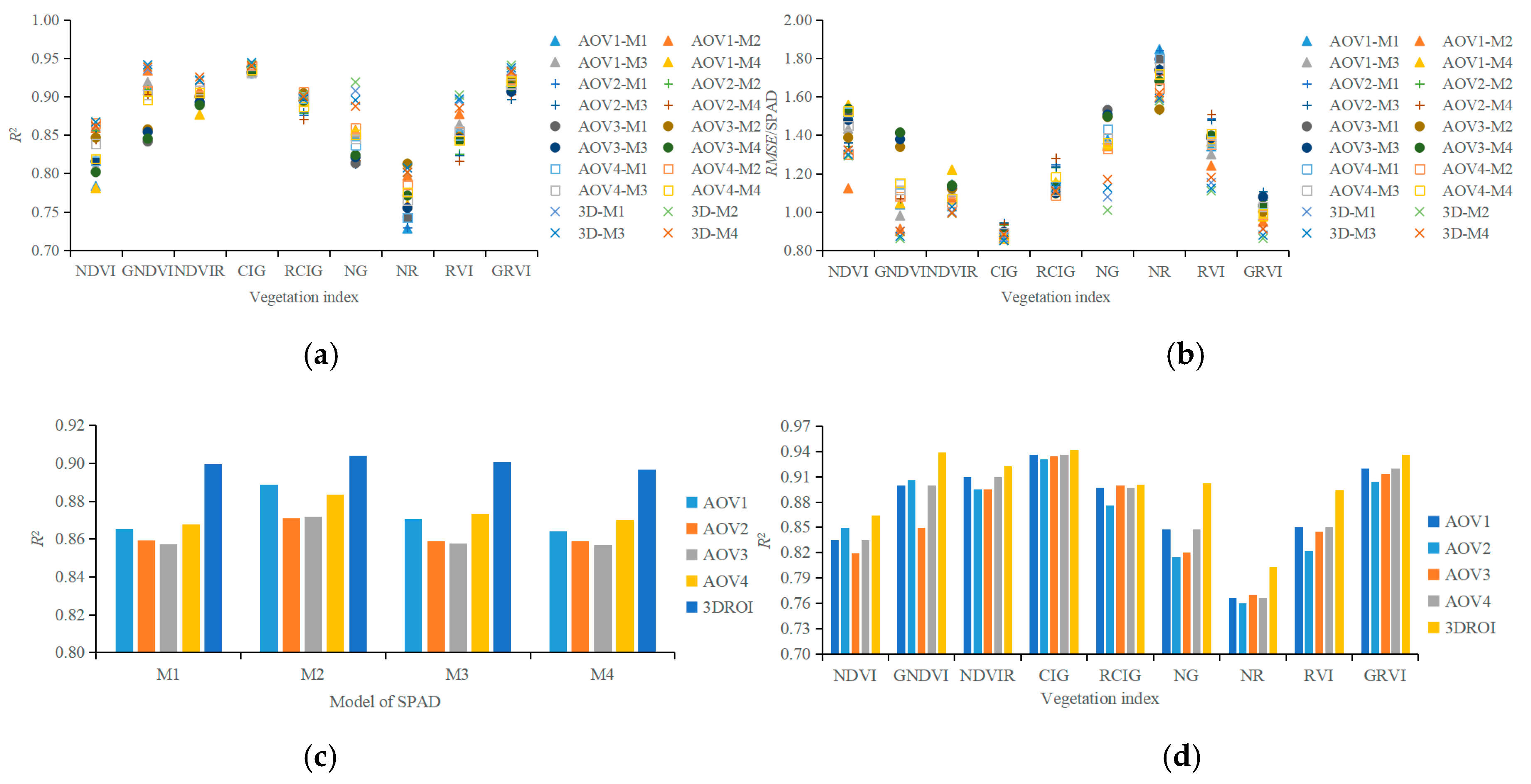
| Vegetable Index | Point Cloud Model | Prototype Function | SPAD Regression Equation | R2 | RMSE |
|---|---|---|---|---|---|
| NDVI | 3DROI | M2 | SPAD = 154.8NDVI2 − 77.053NDVI + 43.256 | 0.8670 | 1.2916 |
| GNDVI | 3DROI | M3 | SPAD = 14.998 × 102.4631GNDVI | 0.9414 | 0.8725 |
| NDVIR | 3DROI | M4 | SPAD = 120.28NDVIR0.5542 | 0.9253 | 0.9940 |
| CIG | 3DROI | M3 | SPAD = 24.001 × 100.333CIG | 0.9443 | 0.8508 |
| RCIG | 3DROI | M2 | SPAD = −18.37RCIG2 + 58.963RCIG + 23.433 | 0.9023 | 1.1066 |
| NG | 3DROI | M2 | SPAD = −2311.2NG2 + 762.19NG − 9.1868 | 0.9188 | 1.008 |
| NR | 3DROI | M3 | SPAD = 122.99 × 10−5.537NR | 0.8071 | 1.5918 |
| RVI | 3DROI | M2 | SPAD = 1.3041RVI2 − 2.805RVI + 35.654 | 0.9019 | 1.1091 |
| GRVI | 3DROI | M2 | SPAD = 5.9953GRVI2 − 19.913GRVI + 51.704 | 0.9408 | 0.8616 |
© 2019 by the authors. Licensee MDPI, Basel, Switzerland. This article is an open access article distributed under the terms and conditions of the Creative Commons Attribution (CC BY) license (http://creativecommons.org/licenses/by/4.0/).
Share and Cite
Sun, G.; Wang, X.; Sun, Y.; Ding, Y.; Lu, W. Measurement Method Based on Multispectral Three-Dimensional Imaging for the Chlorophyll Contents of Greenhouse Tomato Plants. Sensors 2019, 19, 3345. https://doi.org/10.3390/s19153345
Sun G, Wang X, Sun Y, Ding Y, Lu W. Measurement Method Based on Multispectral Three-Dimensional Imaging for the Chlorophyll Contents of Greenhouse Tomato Plants. Sensors. 2019; 19(15):3345. https://doi.org/10.3390/s19153345
Chicago/Turabian StyleSun, Guoxiang, Xiaochan Wang, Ye Sun, Yongqian Ding, and Wei Lu. 2019. "Measurement Method Based on Multispectral Three-Dimensional Imaging for the Chlorophyll Contents of Greenhouse Tomato Plants" Sensors 19, no. 15: 3345. https://doi.org/10.3390/s19153345
APA StyleSun, G., Wang, X., Sun, Y., Ding, Y., & Lu, W. (2019). Measurement Method Based on Multispectral Three-Dimensional Imaging for the Chlorophyll Contents of Greenhouse Tomato Plants. Sensors, 19(15), 3345. https://doi.org/10.3390/s19153345