Depth from a Motion Algorithm and a Hardware Architecture for Smart Cameras


Abstract
1. Introduction
1.1. Depth Estimation from Monocular Sequences
1.2. Motivation and Scope
2. Related Work
2.1. FPGA Architectures for Optical Flow
2.2. Optical Flow Methods Based on Learning Techniques
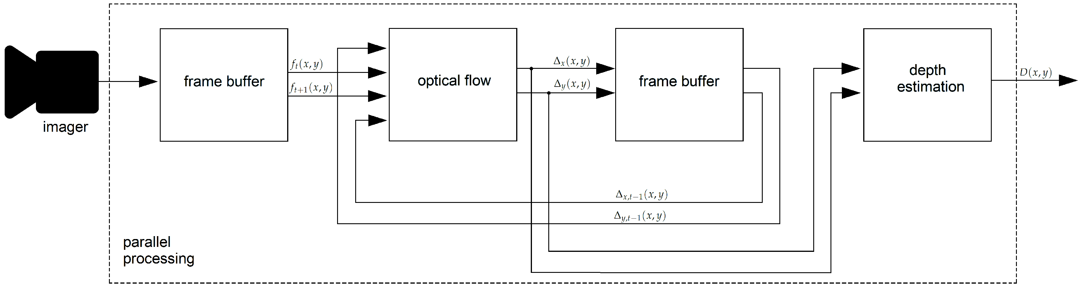
3. The Proposed Algorithm
3.1. Frame Buffer
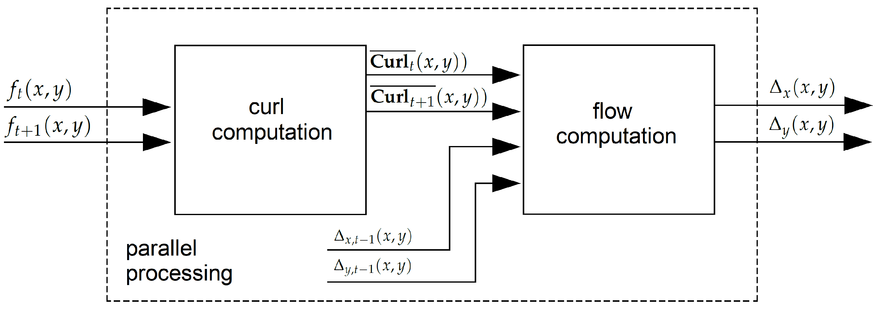
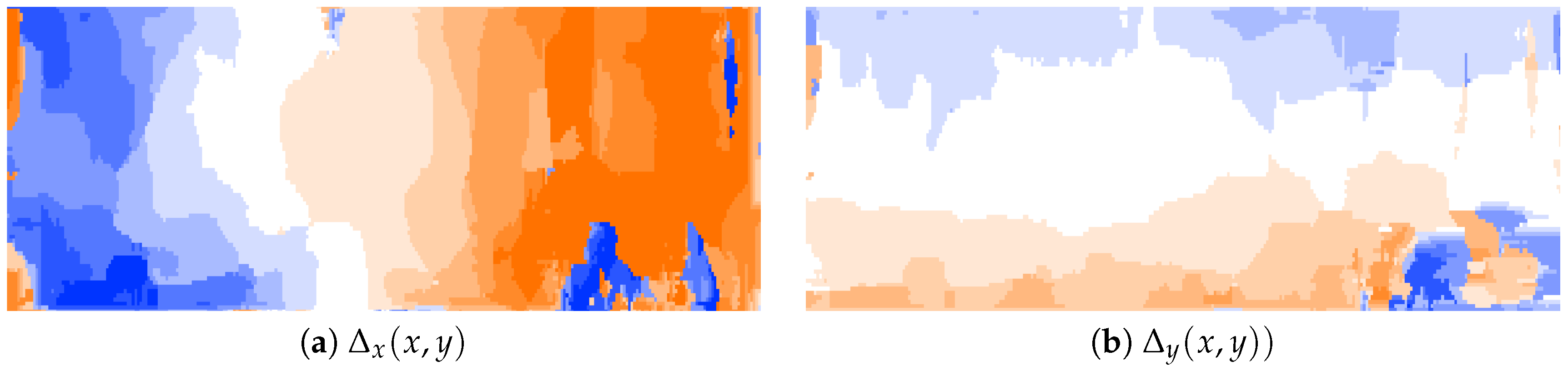
3.2. Optical Flow
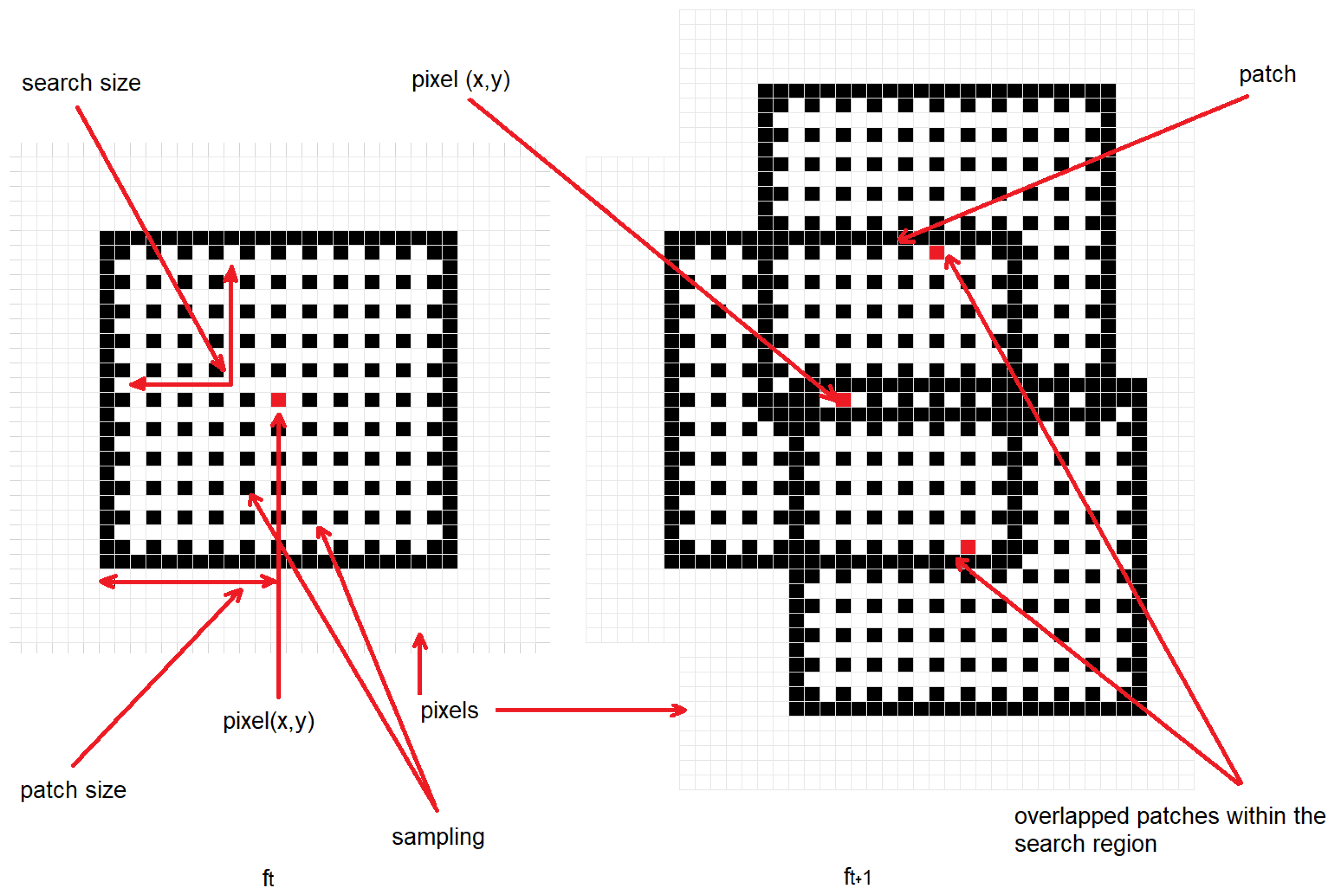
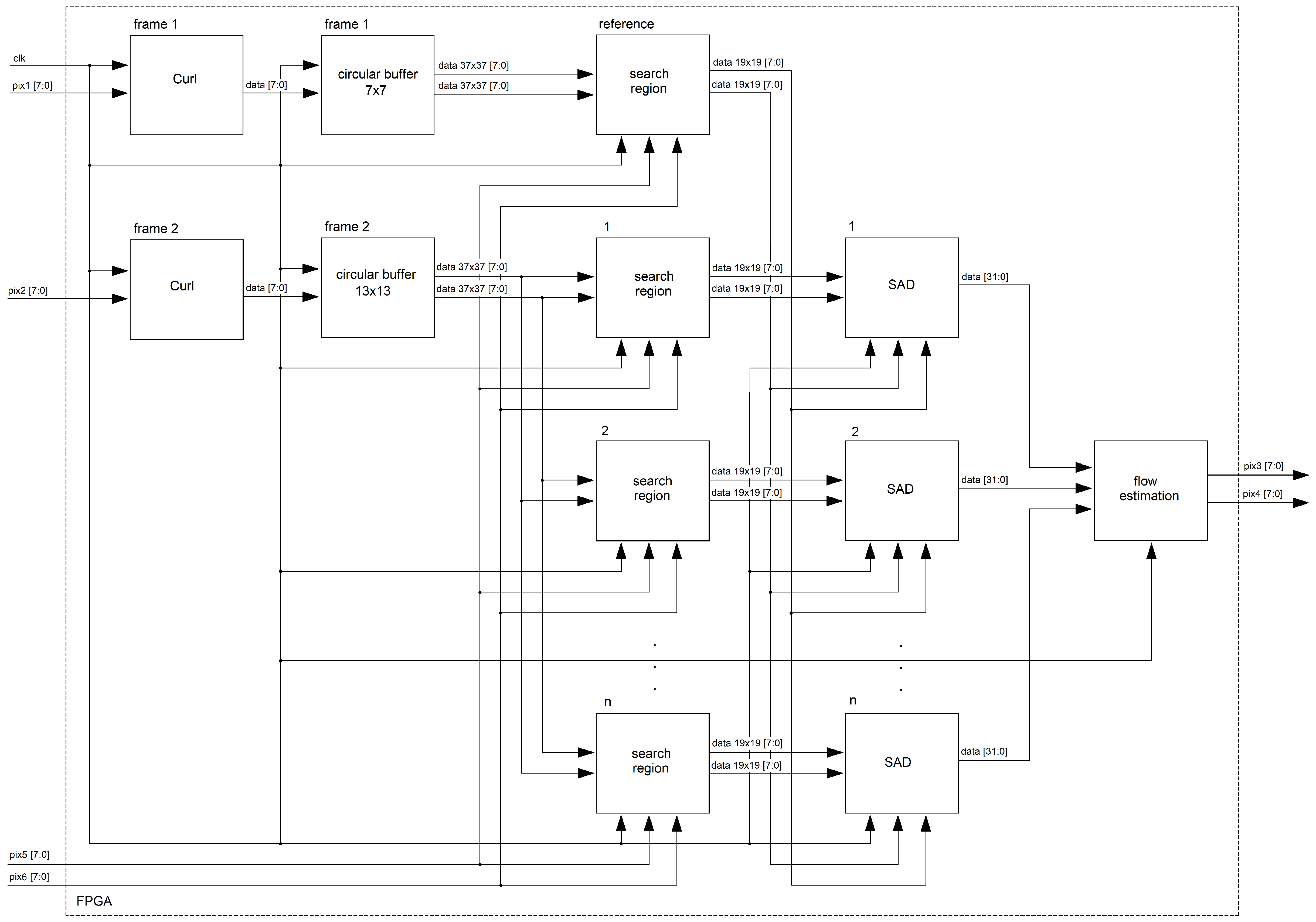
3.3. Search Template
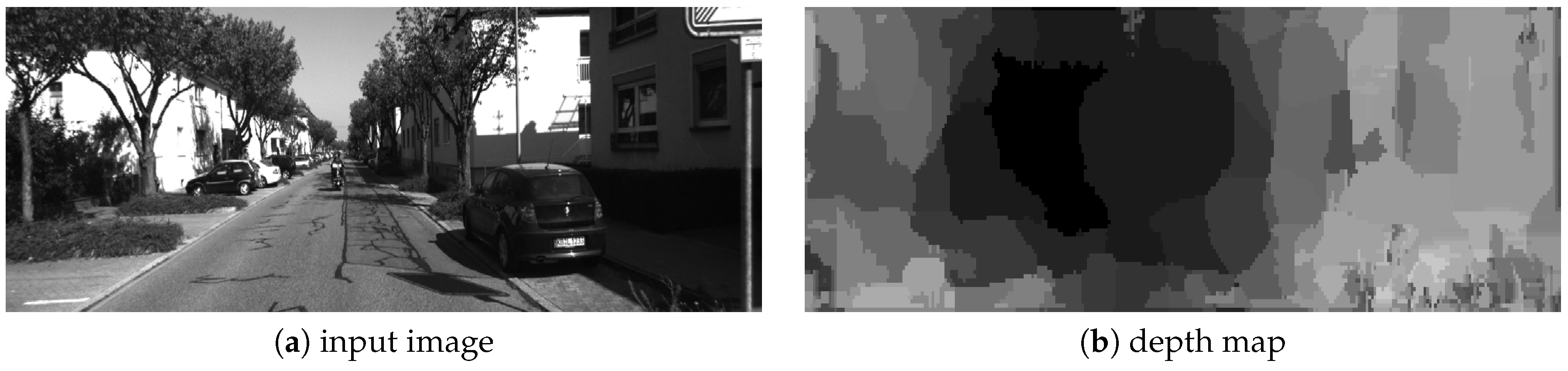
3.4. Depth Estimation
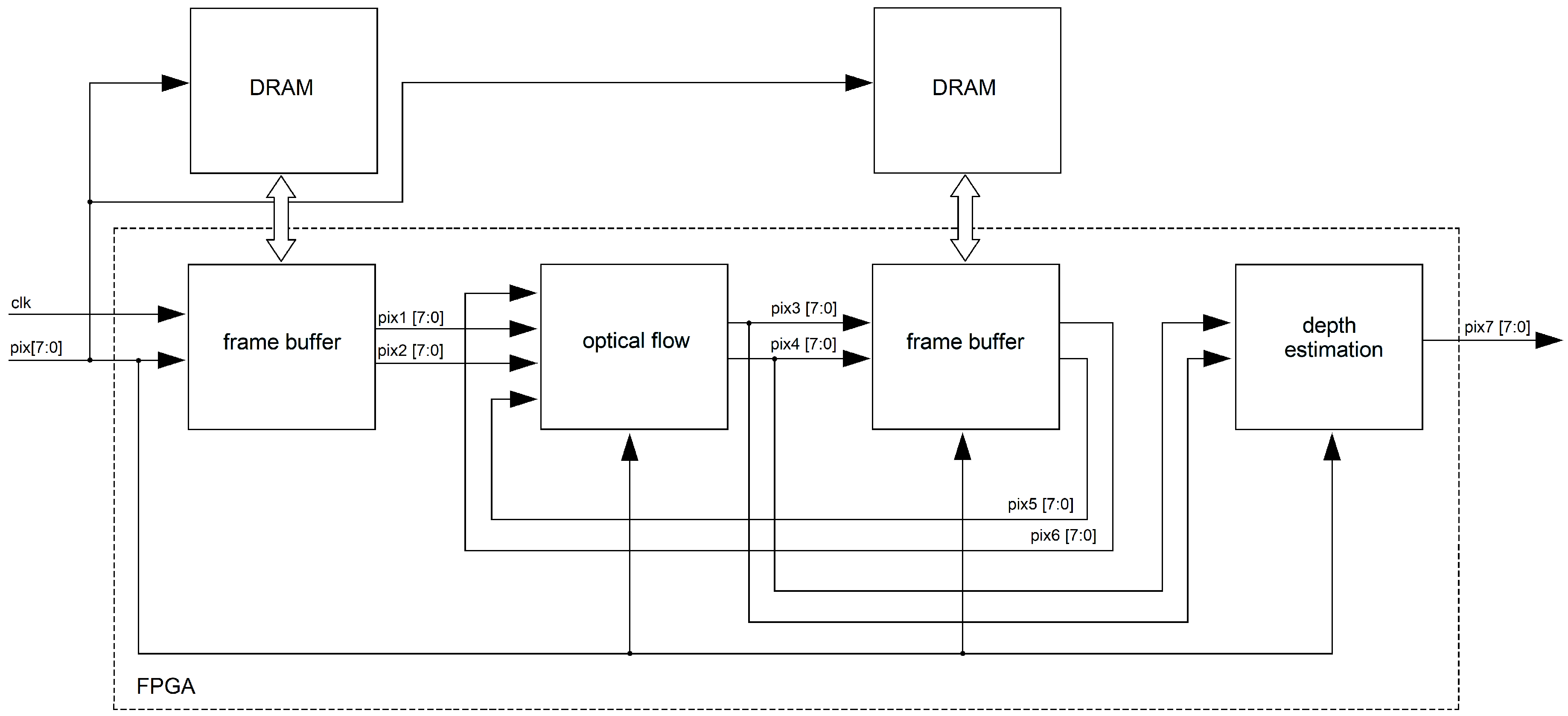
4. The FPGA Architecture
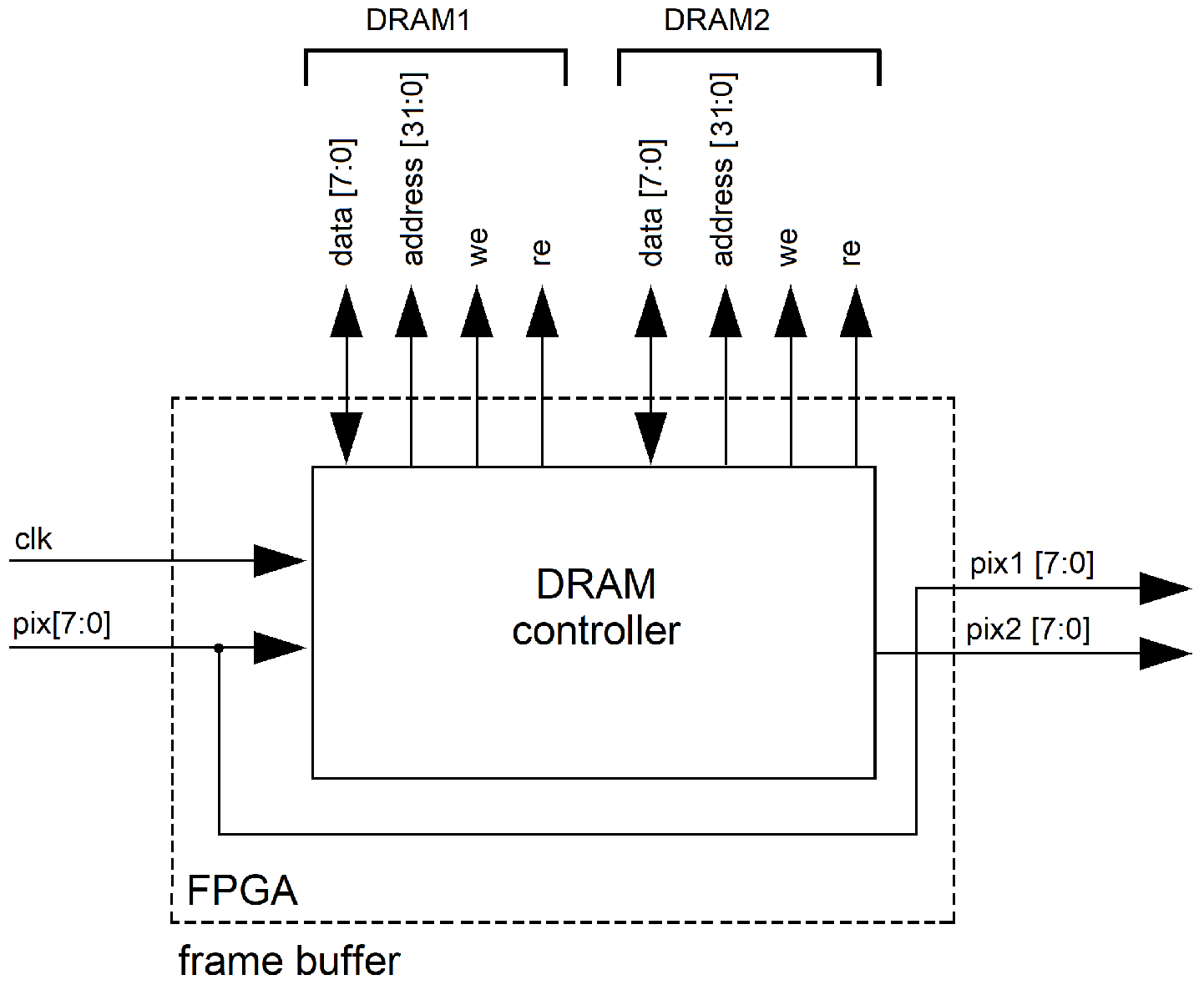
4.1. Frame Buffer
- : DRAM 1 in write mode (storing Frame 1), DRAM 2 in read mode (invalid values), Frame 1 at Output 1, invalid values at Output 2.
- : DRAM 1 in read mode (reading Frame 1), DRAM 2 in write mode (storing Frame 1), Frame 1 at Output 2, Frame 1 at Output 2.
- : DRAM 1 in write mode (storing Frame 3), DRAM 2 in read mode (reading Frame 2), Frame 3 at Output 2, Frame 2 at Output 2 and so on.
4.2. Optical Flow
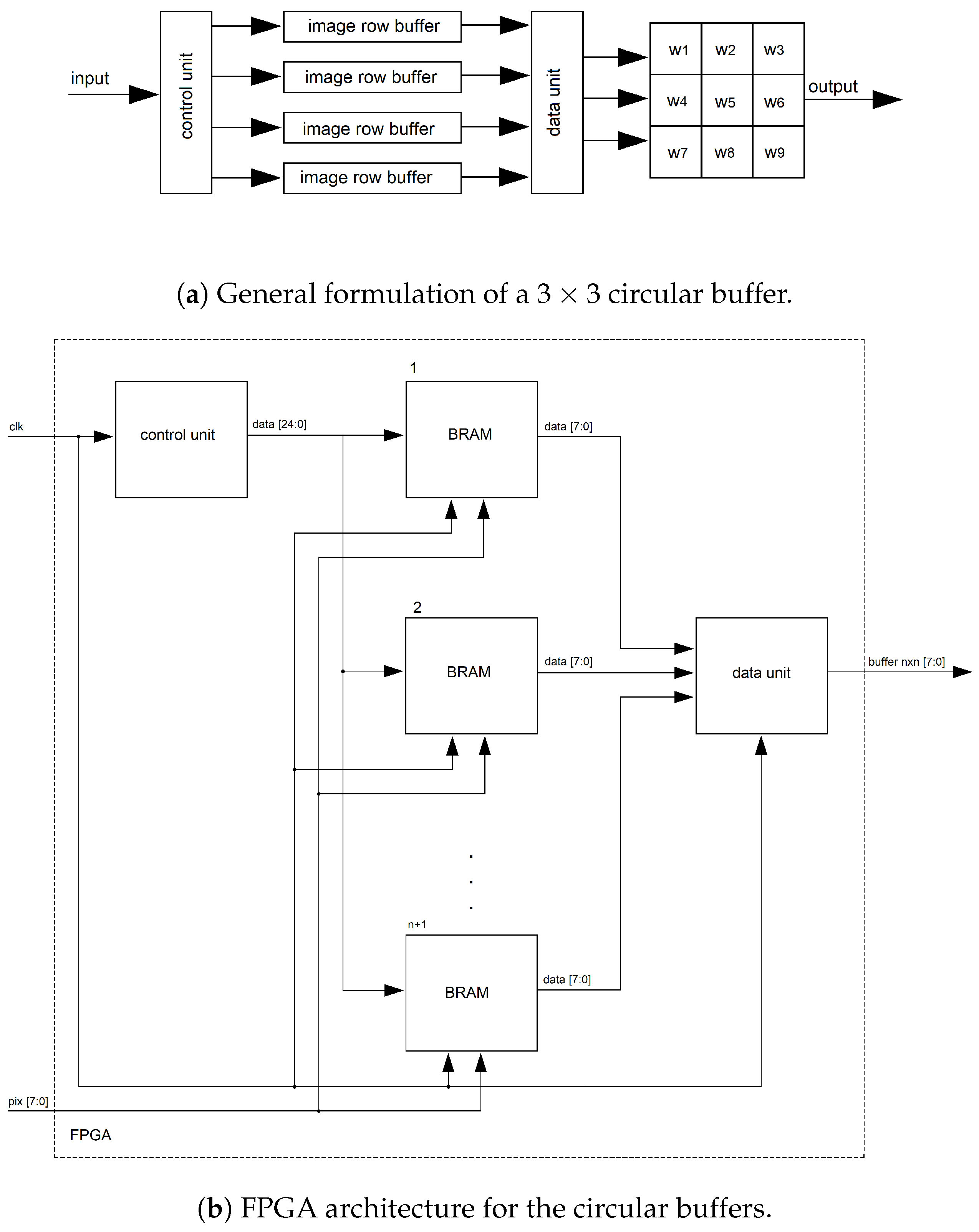
4.2.1. Circular Buffer
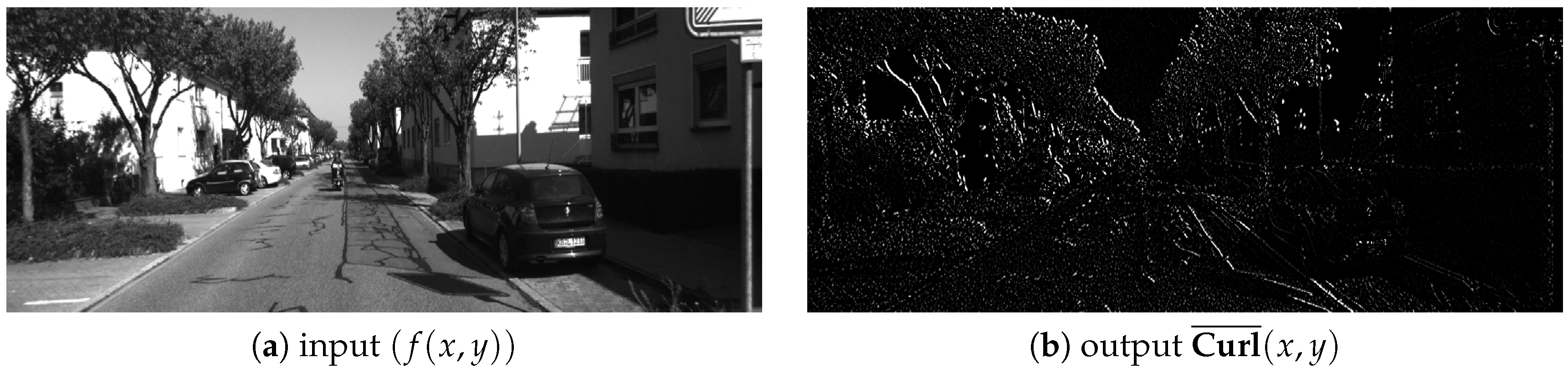
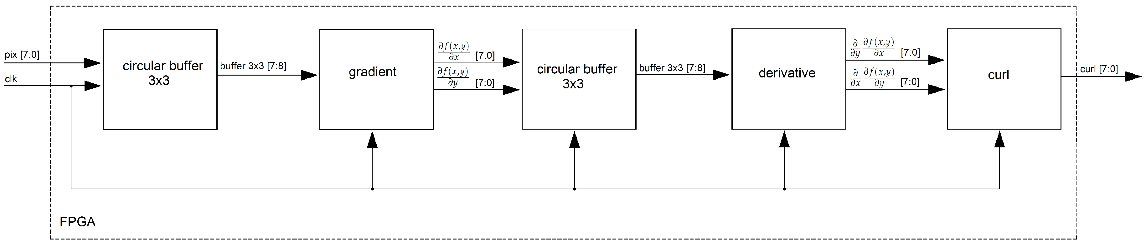
4.2.2. Curl Estimation
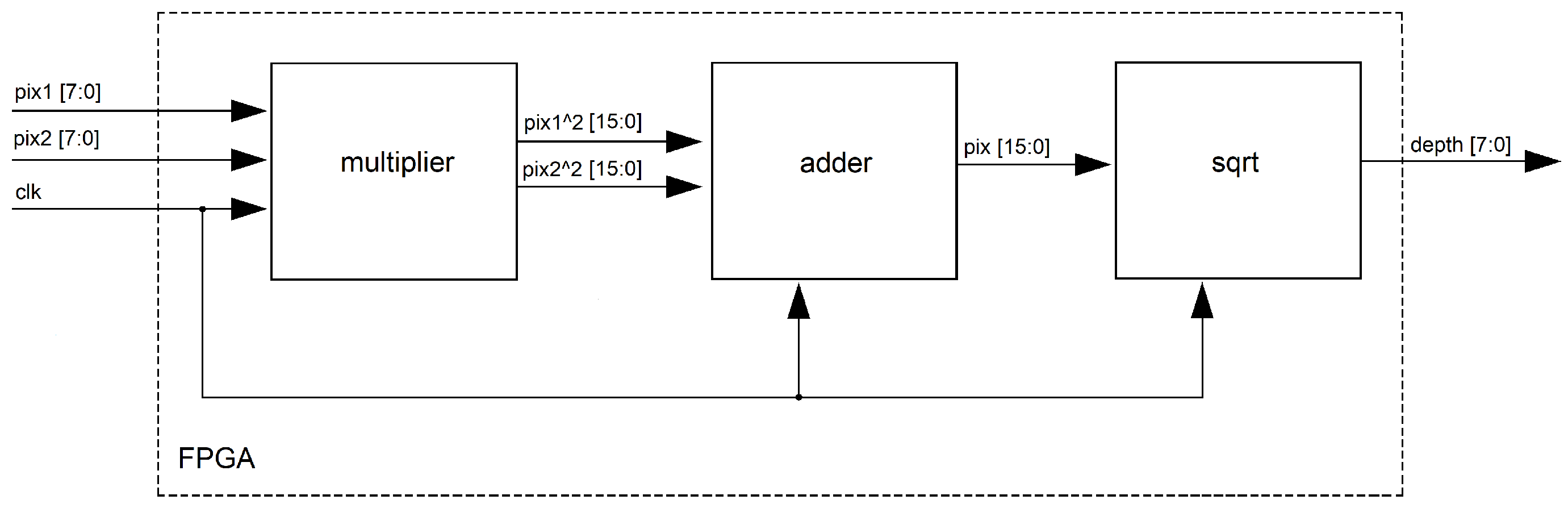
4.3. Depth Estimation
5. Result and Discussion
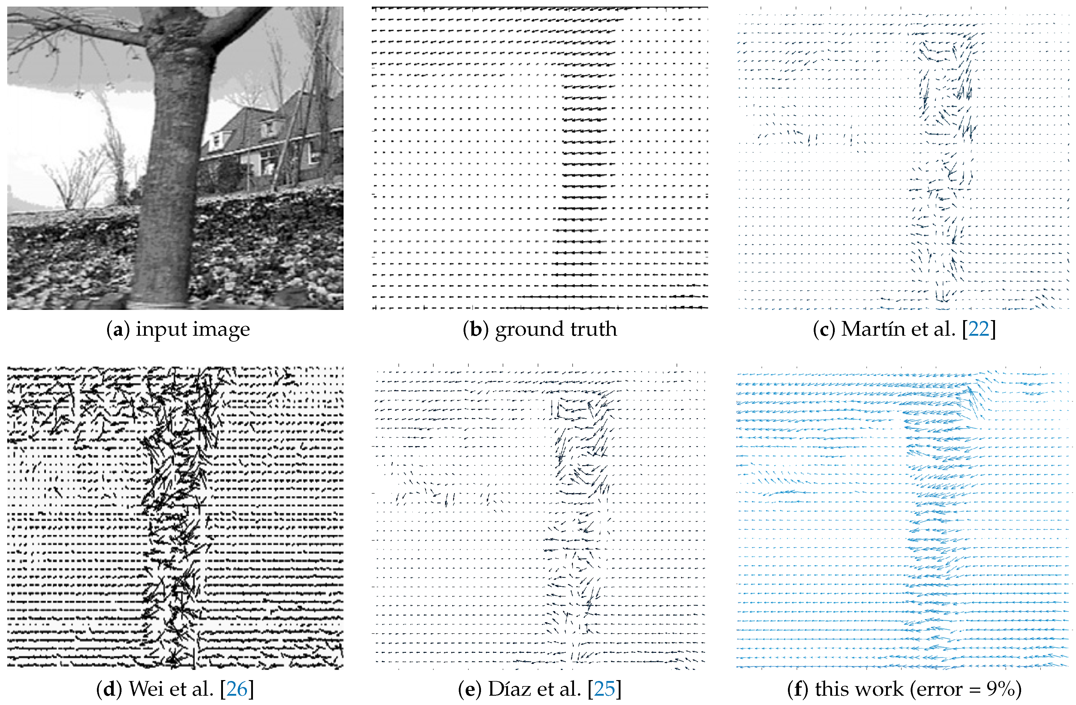
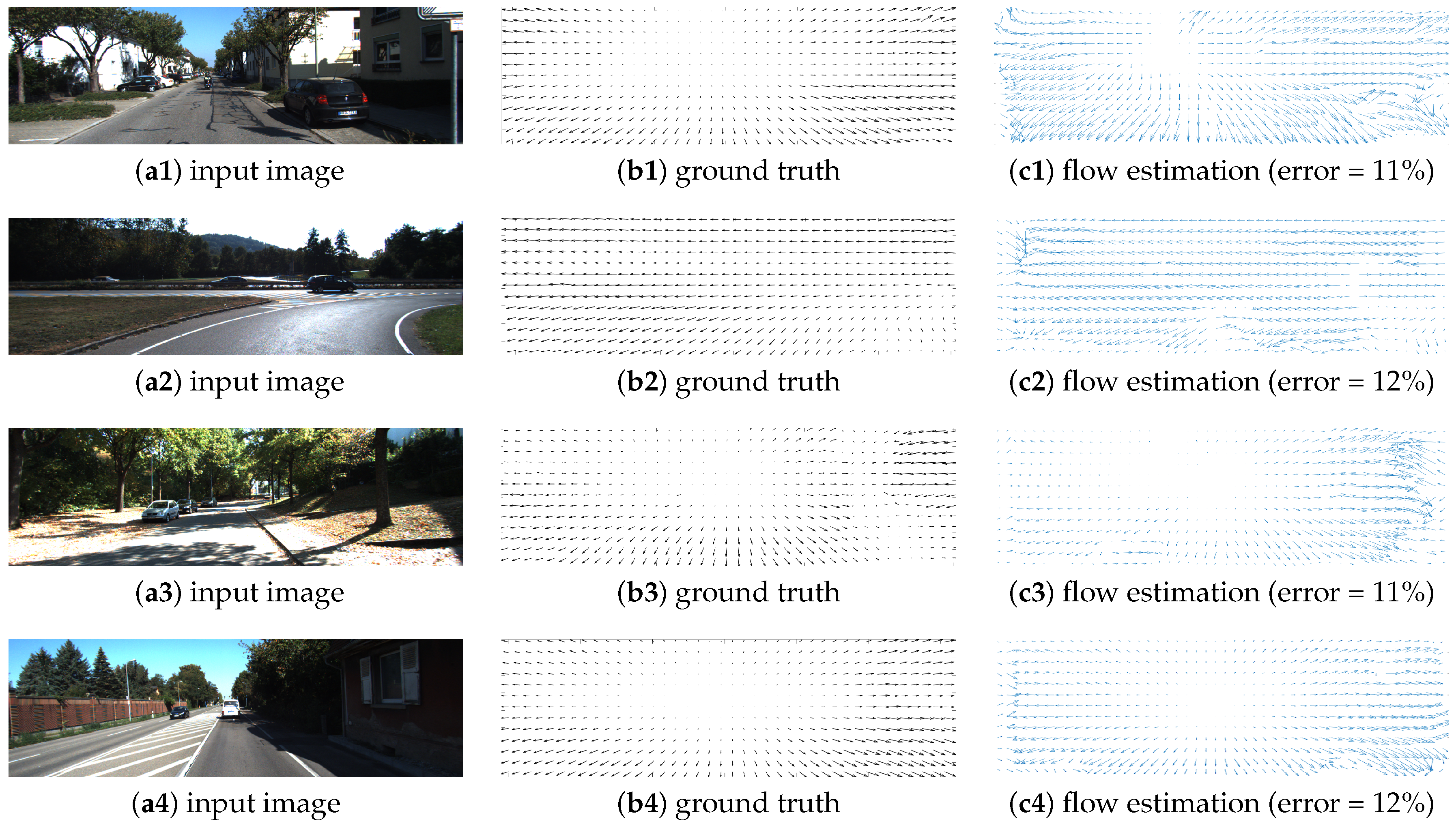
5.1. Performance for the Optical Flow Algorithm
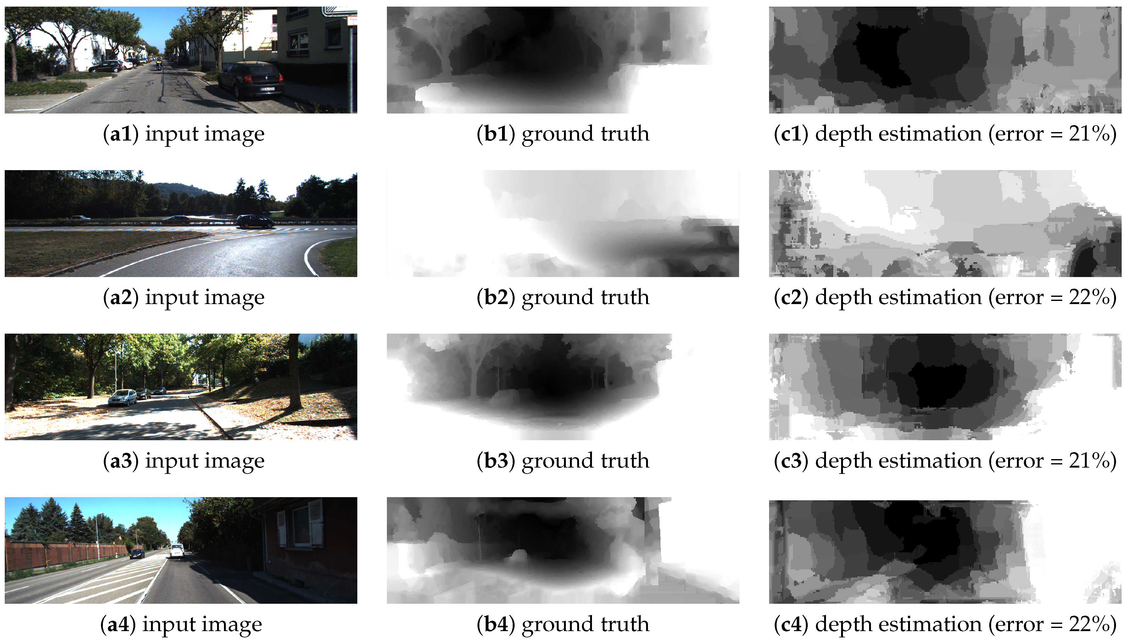
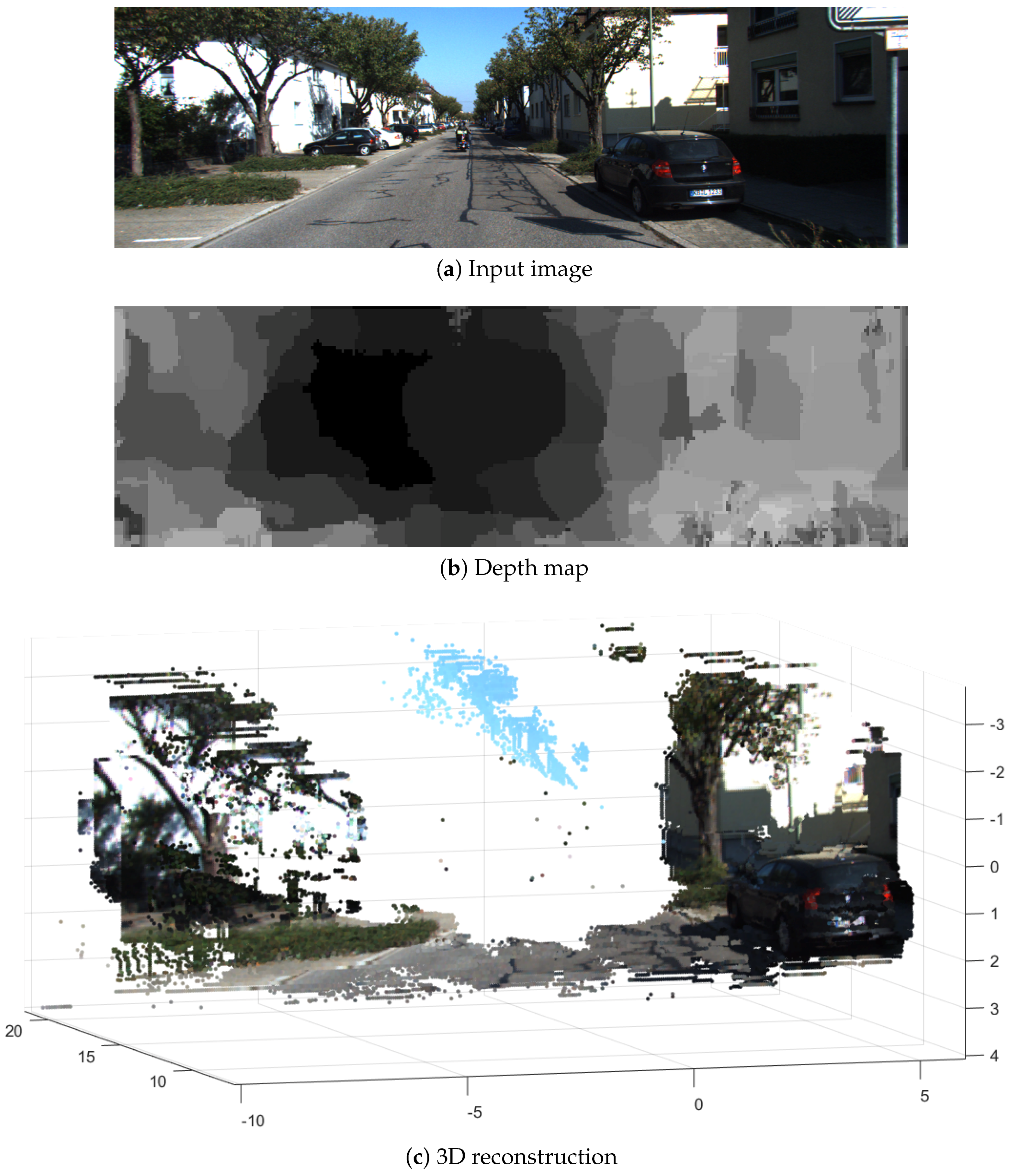
5.2. Performance for the Depth Estimation Step
6. Conclusions
Author Contributions
Funding
Conflicts of Interest
References
- Hengstler, S.; Prashanth, D.; Fong, S.; Aghajan, H. MeshEye: A hybrid-resolution smart camera mote for applications in distributed intelligent surveillance. In Proceedings of the 6th International Conference on Information Processing in Sensor Networks, Cambridge, MA, USA, 25–27 April 2007; pp. 360–369. [Google Scholar]
- Aguilar-González, A.; Arias-Estrada, M. Towards a smart camera for monocular SLAM. In Proceedings of the 10th International Conference on Distributed Smart Camera, Paris, France, 12–15 September 2016; pp. 128–135. [Google Scholar]
- Carey, S.J.; Barr, D.R.; Dudek, P. Low power high-performance smart camera system based on SCAMP vision sensor. J. Syst. Archit. 2013, 59, 889–899. [Google Scholar] [CrossRef]
- Birem, M.; Berry, F. DreamCam: A modular FPGA-based smart camera architecture. J. Syst. Archit. 2014, 60, 519–527. [Google Scholar] [CrossRef]
- Bourrasset, C.; Maggianiy, L.; Sérot, J.; Berry, F.; Pagano, P. Distributed FPGA-based smart camera architecture for computer vision applications. In Proceedings of the 2013 Seventh International Conference on Distributed Smart Cameras (ICDSC), Palm Springs, CA, USA, 29 October–1 November 2013; pp. 1–2. [Google Scholar]
- Bravo, I.; Baliñas, J.; Gardel, A.; Lázaro, J.L.; Espinosa, F.; García, J. Efficient smart cmos camera based on fpgas oriented to embedded image processing. Sensors 2011, 11, 2282–2303. [Google Scholar] [CrossRef] [PubMed]
- Köhler, T.; Röchter, F.; Lindemann, J.P.; Möller, R. Bio-inspired motion detection in an FPGA-based smart camera module. Bioinspir. Biomim. 2009, 4, 015008. [Google Scholar] [CrossRef] [PubMed]
- Olson, T.; Brill, F. Moving object detection and event recognition algorithms for smart cameras. In Proceedings of the DARPA Image Understanding Workshop, New Orleans, LA, USA, 11 May 1997; Volume 20, pp. 205–208. [Google Scholar]
- Norouznezhad, E.; Bigdeli, A.; Postula, A.; Lovell, B.C. Object tracking on FPGA-based smart cameras using local oriented energy and phase features. In Proceedings of the Fourth ACM/IEEE International Conference on Distributed Smart Cameras, Atlanta, GA, USA, 31 August–4 September 2010; pp. 33–40. [Google Scholar]
- Fularz, M.; Kraft, M.; Schmidt, A.; Kasiński, A. The architecture of an embedded smart camera for intelligent inspection and surveillance. In Progress in Automation, Robotics and Measuring Techniques; Springer: Berlin, Germany, 2015; pp. 43–52. [Google Scholar]
- Haritaoglu, I.; Harwood, D.; Davis, L.S. W 4: Real-time surveillance of people and their activities. IEEE Trans. Pattern Anal. Mach. Intell. 2000, 22, 809–830. [Google Scholar] [CrossRef]
- Biswas, J.; Veloso, M. Depth camera based indoor mobile robot localization and navigation. In Proceedings of the 2012 IEEE International Conference on Robotics and Automation, Saint Paul, MN, USA, 14–18 May 2012; pp. 1697–1702. [Google Scholar]
- Stowers, J.; Hayes, M.; Bainbridge-Smith, A. Altitude control of a quadrotor helicopter using depth map from Microsoft Kinect sensor. In Proceedings of the 2011 IEEE International Conference on Mechatronics, Istanbul, Turkey, 13–15 April 2011; pp. 358–362. [Google Scholar]
- Scharstein, D.; Szeliski, R. A taxonomy and evaluation of dense two-frame stereo correspondence algorithms. Int. J. Comput. Vis. 2002, 47, 7–42. [Google Scholar] [CrossRef]
- Subbarao, M.; Surya, G. Depth from defocus: A spatial domain approach. Int. J. Comput. Vis. 1994, 13, 271–294. [Google Scholar] [CrossRef]
- Chen, Y.; Alain, M.; Smolic, A. Fast and accurate optical flow based depth map estimation from light fields. In Proceedings of the Irish Machine Vision and Image Processing Conference (IMVIP), Maynooth, Ireland, 30 August–1 September 2017. [Google Scholar]
- Zhang, J.; Singh, S. Visual-lidar odometry and mapping: Low-drift, robust, and fast. In Proceedings of the 2015 IEEE International Conference on Robotics and Automation (ICRA), Seattle, WA, USA, 26–30 May 2015; pp. 2174–2181. [Google Scholar]
- Schubert, S.; Neubert, P.; Protzel, P. Towards camera based navigation in 3d maps by synthesizing depth images. In Proceedings of the Annual Conference Towards Autonomous Robotic Systems, Guildford, UK, 19–21 July 2017; Springer: Berlin, Germany, 2017; pp. 601–616. [Google Scholar]
- Maddern, W.; Newman, P. Real-time probabilistic fusion of sparse 3d lidar and dense stereo. In Proceedings of the 2016 IEEE/RSJ International Conference on Intelligent Robots and Systems (IROS), Daejeon, Korea, 9–14 October 2016; pp. 2181–2188. [Google Scholar]
- Dai, A.; Chang, A.X.; Savva, M.; Halber, M.; Funkhouser, T.A.; Nießner, M. ScanNet: Richly-Annotated 3D Reconstructions of Indoor Scenes. In Proceedings of the Conference on Computer Vision and Pattern Recognition, Honolulu, HI, USA, 21–26 July 2017; Volume 2, p. 10. [Google Scholar]
- Liu, H.; Li, C.; Chen, G.; Zhang, G.; Kaess, M.; Bao, H. Robust Keyframe-Based Dense SLAM with an RGB-D Camera. arXiv, 2017; arXiv:1711.05166. [Google Scholar]
- Martín, J.L.; Zuloaga, A.; Cuadrado, C.; Lázaro, J.; Bidarte, U. Hardware implementation of optical flow constraint equation using FPGAs. Comput. Vis. Image Underst. 2005, 98, 462–490. [Google Scholar] [CrossRef]
- Aguilar-González, A.; Arias-Estrada, M.; Pérez-Patricio, M.; Camas-Anzueto, J. An FPGA 2D-convolution unit based on the CAPH language. J. Real-Time Image Process. 2015, 1–15. [Google Scholar] [CrossRef]
- Pérez-Patricio, M.; Aguilar-González, A.; Arias-Estrada, M.; Hernandez-de Leon, H.R.; Camas-Anzueto, J.L.; de Jesús Osuna-Coutiño, J. An FPGA stereo matching unit based on fuzzy logic. Microprocess. Microsyst. 2016, 42, 87–99. [Google Scholar] [CrossRef]
- Díaz, J.; Ros, E.; Pelayo, F.; Ortigosa, E.M.; Mota, S. FPGA-based real-time optical-flow system. IEEE Trans. Circuits Syst. Video Technol. 2006, 16, 274–279. [Google Scholar] [CrossRef]
- Wei, Z.; Lee, D.J.; Nelson, B.E. FPGA-based Real-time Optical Flow Algorithm Design and Implementation. J. Multimed. 2007, 2, 38–45. [Google Scholar] [CrossRef]
- Barranco, F.; Tomasi, M.; Diaz, J.; Vanegas, M.; Ros, E. Parallel architecture for hierarchical optical flow estimation based on FPGA. IEEE Trans. Very Large Scale Integr. Syst. 2012, 20, 1058–1067. [Google Scholar] [CrossRef]
- Tomasi, C.; Kanade, T. Detection and Tracking of Point Features; School of Computer Science, Carnegie Mellon University: Pittsburgh, PA, USA, 1991. [Google Scholar]
- Honegger, D.; Greisen, P.; Meier, L.; Tanskanen, P.; Pollefeys, M. Real-time velocity estimation based on optical flow and disparity matching. In Proceedings of the IEEE/RSJ International Conference on Intelligent Robots and Systems, Vilamoura, Portugal, 7–12 October 2012; pp. 5177–5182. [Google Scholar]
- Chao, H.; Gu, Y.; Napolitano, M. A survey of optical flow techniques for robotics navigation applications. J. Intell. Robot. Syst. 2014, 73, 361–372. [Google Scholar] [CrossRef]
- Dosovitskiy, A.; Fischer, P.; Ilg, E.; Hausser, P.; Hazirbas, C.; Golkov, V.; Van Der Smagt, P.; Cremers, D.; Brox, T. Flownet: Learning optical flow with convolutional networks. In Proceedings of the IEEE International Conference on Computer Vision, Santiago, Chile, 11–18 December 2015; pp. 2758–2766. [Google Scholar]
- Ilg, E.; Mayer, N.; Saikia, T.; Keuper, M.; Dosovitskiy, A.; Brox, T. Flownet 2.0: Evolution of optical flow estimation with deep networks. In Proceedings of the IEEE Conference on Computer Vision and Pattern Recognition (CVPR), Honolulu, HI, USA, 21–26 July 2017; Volume 2, p. 6. [Google Scholar]
- Horn, B.K.; Schunck, B.G. Determining optical flow. Artif. Intell. 1981, 17, 185–203. [Google Scholar] [CrossRef]
- Khaleghi, B.; Shahabi, S.M.A.; Bidabadi, A. Performace evaluation of similarity metrics for stereo corresponce problem. In Proceedings of the Canadian Conference on Electrical and Computer Engineering, Vancouver, BC, Canada, 22–26 April 2007; pp. 1476–1478. [Google Scholar]
- Geiger, A.; Lenz, P.; Stiller, C.; Urtasun, R. Vision meets robotics: The KITTI dataset. Int. J. Robot. Res. 2013, 32, 1231–1237. [Google Scholar] [CrossRef]
- Baker, S.; Scharstein, D.; Lewis, J.; Roth, S.; Black, M.J.; Szeliski, R. A database and evaluation methodology for optical flow. Int. J. Comput. Vis. 2011, 92, 1–31. [Google Scholar] [CrossRef]
- Fortun, D.; Bouthemy, P.; Kervrann, C. Optical flow modeling and computation: A survey. Comput. Vis. Image Underst. 2015, 134, 1–21. [Google Scholar] [CrossRef]
- Li, Y.; Chu, W. A new non-restoring square root algorithm and its VLSI implementations. In Proceedings of the IEEE International Conference on Computer Design: VLSI in Computers and Processors, Austin, TX, USA, 7–9 October 1996; pp. 538–544. [Google Scholar]
- Fu, H.; Gong, M.; Wang, C.; Batmanghelich, K.; Tao, D. Deep Ordinal Regression Network for Monocular Depth Estimation. In Proceedings of the IEEE Conference on Computer Vision and Pattern Recognition (CVPR), Salt Lake City, UT, USA, 18–22 June 2018. [Google Scholar]
- Li, B.; Dai, Y.; He, M. Monocular Depth Estimation with Hierarchical Fusion of Dilated CNNs and Soft-Weighted-Sum Inference. Pattern Recognit. 2018, 83, 328–339. [Google Scholar] [CrossRef]
- Zhou, T.; Brown, M.; Snavely, N.; Lowe, D.G. Unsupervised learning of depth and ego-motion from video. In Proceedings of the 2017 Conference on Computer Vision and Pattern Recognition, Honolulu, HI, USA, 21–26 July 2017; Volume 2, p. 7. [Google Scholar]
- Yang, Z.; Wang, P.; Wang, Y.; Xu, W.; Nevatia, R. LEGO: Learning Edge with Geometry All at Once by Watching Videos. In Proceedings of the IEEE Conference on Computer Vision and Pattern Recognition, Salt Lake City, UT, USA, 18–22 June 2018; pp. 225–234. [Google Scholar]
- Godard, C.; Mac Aodha, O.; Brostow, G. Digging Into Self-Supervised Monocular Depth Estimation. arXiv, 2018; arXiv:1806.01260. [Google Scholar]
- Uhrig, J.; Schneider, N.; Schneider, L.; Franke, U.; Brox, T.; Geiger, A. Depth Prediction Evaluation. 2017. Available online: http://www.cvlibs.net/datasets/kitti/eval_odometry_detail.php?&result=fee1ecc5afe08bc002f093b48e9ba98a295a79ed (accessed on 15 March 2012).
- Yang, Z.; Wang, P.; Xu, W.; Zhao, L.; Nevatia, R. Unsupervised Learning of Geometry with Edge-Aware Depth-Normal Consistency. arXiv, 2017; arXiv:1711.03665. [Google Scholar]
- Mahjourian, R.; Wicke, M.; Angelova, A. Unsupervised Learning of Depth and Ego-Motion from Monocular Video Using 3D Geometric Constraints. In Proceedings of the IEEE Conference on Computer Vision and Pattern Recognition, Salt Lake City, UT, USA, 18–22 June 2018; pp. 5667–5675. [Google Scholar]
- Zou, Y.; Luo, Z.; Huang, J.B. Df-net: Unsupervised joint learning of depth and flow using cross-task consistency. In Proceedings of the European Conference on Computer Vision, Munich, Germany, 8–14 September 2018; Springer: Berlin, Germany, 2018; pp. 38–55. [Google Scholar]
- Mur-Artal, R.; Montiel, J.M.M.; Tardos, J.D. ORB-SLAM: A versatile and accurate monocular SLAM system. IEEE Trans. Robot. 2015, 31, 1147–1163. [Google Scholar] [CrossRef]
- Engel, J.; Schöps, T.; Cremers, D. LSD-SLAM: Large-scale direct monocular SLAM. In Proceedings of the European Conference on Computer Vision, Zurich, Switzerland, 6–12 September 2014; Springer: Berlin, Germany, 2014; pp. 834–849. [Google Scholar]


| Resource | Consumption/Image Resolution | ||
|---|---|---|---|
| 640 × 480 | 320 × 240 | 256 × 256 | |
| Total logic elements | 69,879 (59%) | 37,059 (31%) | 21,659 (18%) |
| Total pins | 16 (3%) | 16 (3%) | 16 (3%) |
| Total Memory Bits | 618,392 (15%) | 163,122 (4%) | 85,607 (2%) |
| Embedded multiplier elements | 0 (0%) | 0 (0%) | 0 (0%) |
| Total PLLs | 1 (25%) | 1 (25%) | 1 (25%) |
| Method | Logic Elements | Memory Bits | Image Resolution |
|---|---|---|---|
| Martín et al. [22] (2005) | 11,520 | 147,456 | 256 × 256 |
| Díaz et al. [25] (2006) | 513,216 | 685,670 | 320 × 240 |
| Wei et al. [26] (2007) | 10,288 | 256 MB (DDR) | 640 × 480 |
| Barranco et al. [27] (2012) | 82,526 | 573,440 | 640 × 480 |
| Honegger et al. [29] (2012) | 49,655 | 1,111,000 | 376 × 240 |
| Our work * | 69,879 | 624,244 | 640 × 480 |
| Our work * | 37,059 | 163,122 | 320 × 240 |
| Our work * | 21,659 | 85,607 | 256 × 256 |
| Resolution | Frames/s | Pixels/s |
|---|---|---|
| 1280 × 1024 | 68 | 90,129,200 |
| 640 × 480 | 297 | 91,238,400 |
| 320 × 240 | 1209 | 92,880,000 |
| 256 × 256 | 1417 | 92,876,430 |
| Method | Resolution | Frames/s | Pixels/s |
|---|---|---|---|
| Martín et al. [22] | 256 × 256 | 60 | 3,932,160 |
| Díaz et al. [25] | 320 × 240 | 30 | 2,304,000 |
| Wei et al. [26] | 640 × 480 | 64 | 19,550,800 |
| Barranco et al. [27] | 640 × 480 | 31 | 9,523,200 |
| Honegger et al. [29] | 376 × 240 | 127 | 11,460,480 |
| Our work | 640 × 480 | 297 | 91,238,400 |
| Method | Error (RMS) | Speed | Image Resolution | Approach | |
|---|---|---|---|---|---|
| Zhou et al. [41] (2017) | 6.8% | - | 128 × 416 | DfM-based * | - |
| Yang et al. [45] (2017) | 6.5% | 5 fps | 128 × 416 | CNN-based * | GTX 1080 (GPU) |
| Mahjourian et al. [46] (2018) | 6.2% | 100 fps | 128 × 416 | DfM-based * | Titan X (GPU) |
| Yang et al. [42] (2018) | 6.2% | - | 830 × 254 | DfM-based * | Titan X (GPU) |
| Godard et al. [43] (2018) | 5.6% | - | 192 × 640 | CNN-based * | - |
| Zou et al. [47] (2018) | 5.6% | 1.25 fps | 576 × 160 | DfM-based * | Tesla K80 (GPU) |
| Our work | 21.5% | 192 fps | 1241 × 376 | DfM-based * | Cyclone IV (FPGA) |
© 2018 by the authors. Licensee MDPI, Basel, Switzerland. This article is an open access article distributed under the terms and conditions of the Creative Commons Attribution (CC BY) license (http://creativecommons.org/licenses/by/4.0/).
Share and Cite
Aguilar-González, A.; Arias-Estrada, M.; Berry, F. Depth from a Motion Algorithm and a Hardware Architecture for Smart Cameras. Sensors 2019, 19, 53. https://doi.org/10.3390/s19010053
Aguilar-González A, Arias-Estrada M, Berry F. Depth from a Motion Algorithm and a Hardware Architecture for Smart Cameras. Sensors. 2019; 19(1):53. https://doi.org/10.3390/s19010053
Chicago/Turabian StyleAguilar-González, Abiel, Miguel Arias-Estrada, and François Berry. 2019. "Depth from a Motion Algorithm and a Hardware Architecture for Smart Cameras" Sensors 19, no. 1: 53. https://doi.org/10.3390/s19010053
APA StyleAguilar-González, A., Arias-Estrada, M., & Berry, F. (2019). Depth from a Motion Algorithm and a Hardware Architecture for Smart Cameras. Sensors, 19(1), 53. https://doi.org/10.3390/s19010053