Incremental 3D Cuboid Modeling with Drift Compensation

 , ,
, ,
Abstract
:1. Introduction
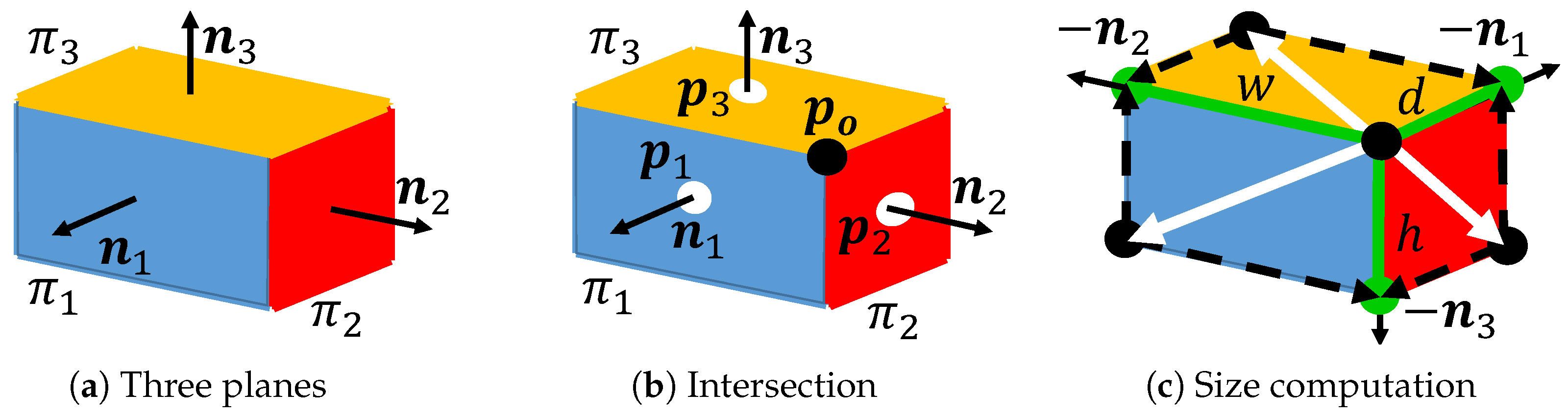
- Cuboid reconstruction is performed by searching three perpendicular planes and computing the intersection of the planes.
- A novel framework for incremental cuboid modeling based on cuboid detection and mapping is proposed.
- The drift error of the SLAM is accurately compensated by using cuboids.
- An application for AR-based interactive cuboid modeling is presented.
2. Related Work
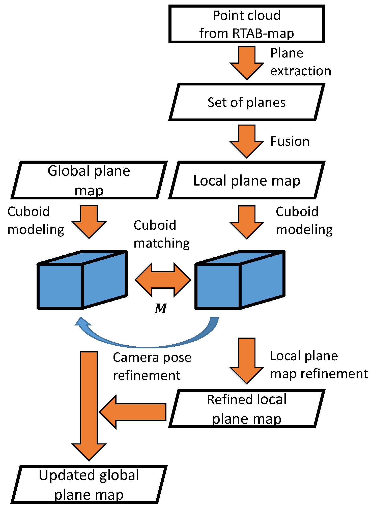
3. Overview
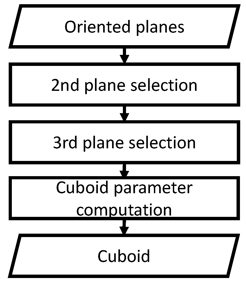
4. Cuboid Detection
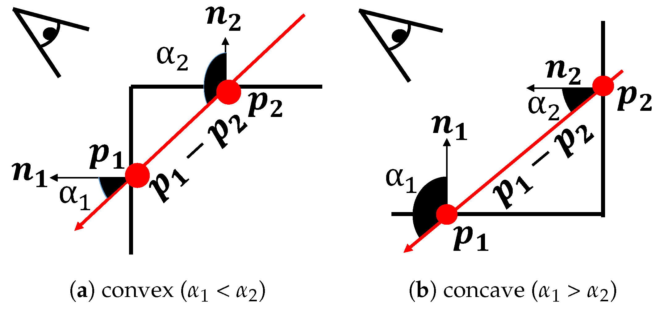
4.1. Second Plane Selection
4.2. Third Plane Selection
4.3. Cuboid Parameter Estimation
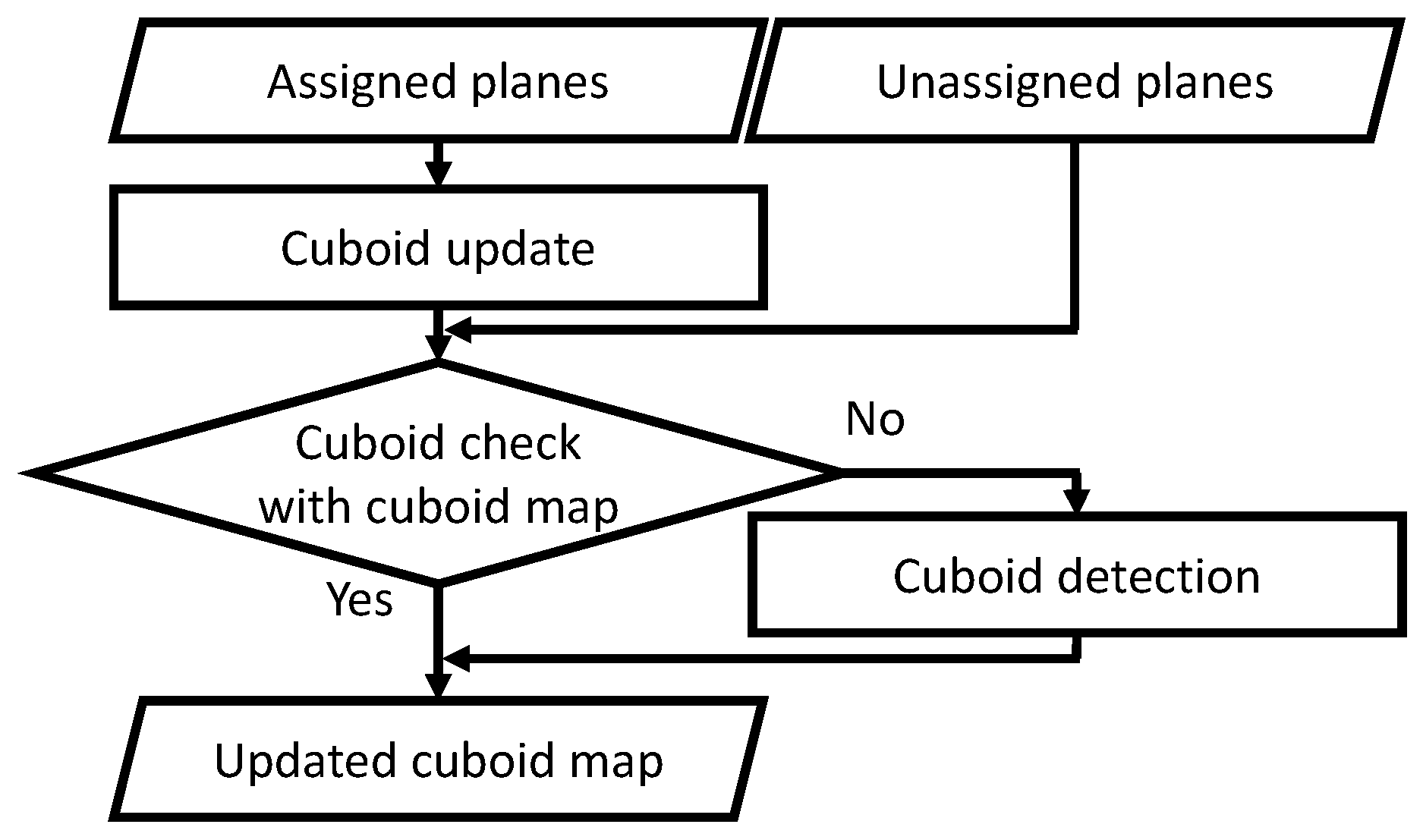
5. Cuboid Mapping
5.1. Cuboid Update
5.2. Cuboid Check with Cuboid Map
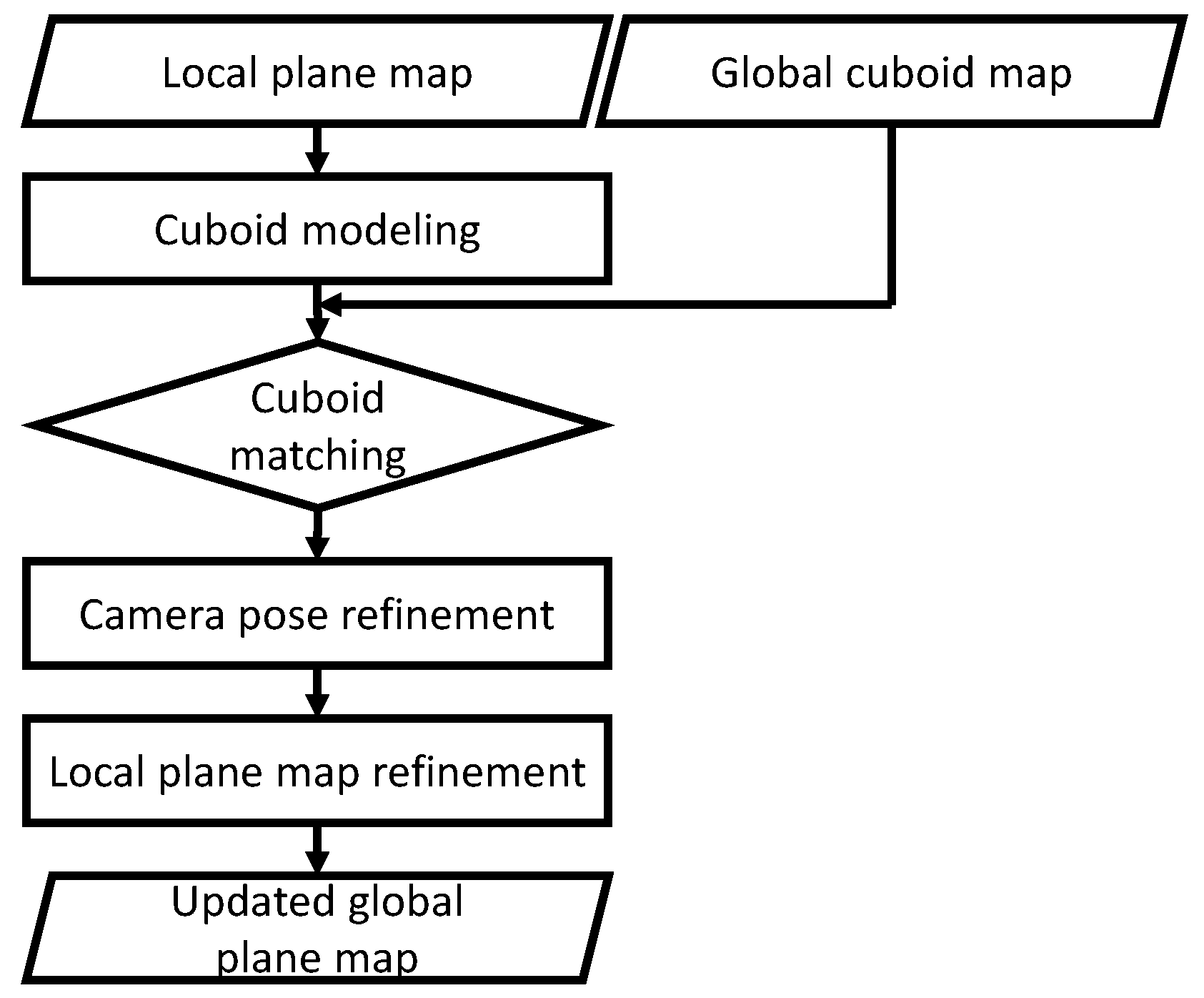
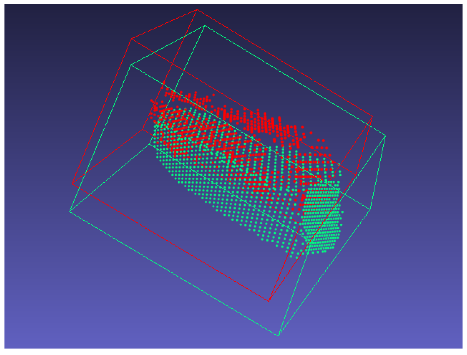
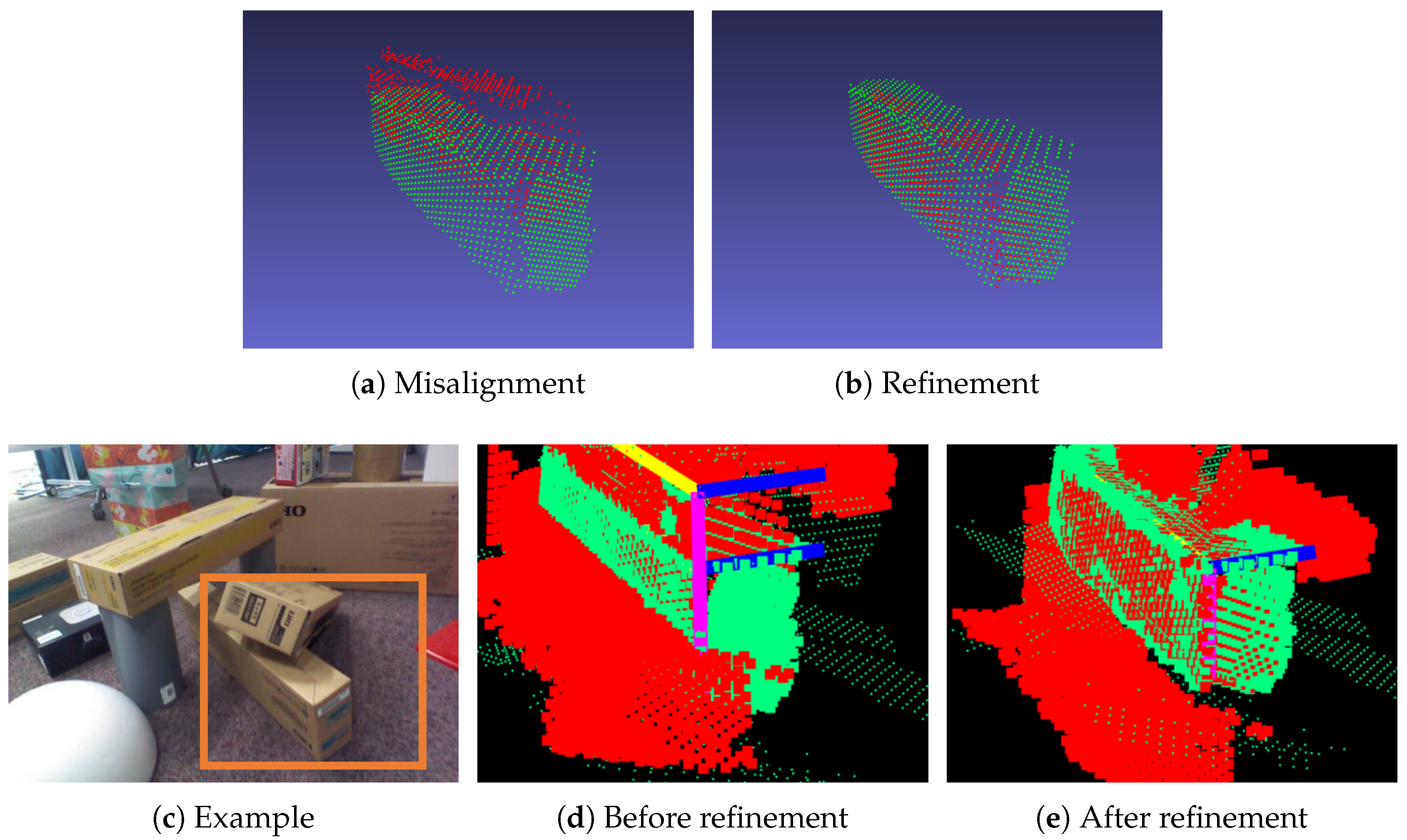
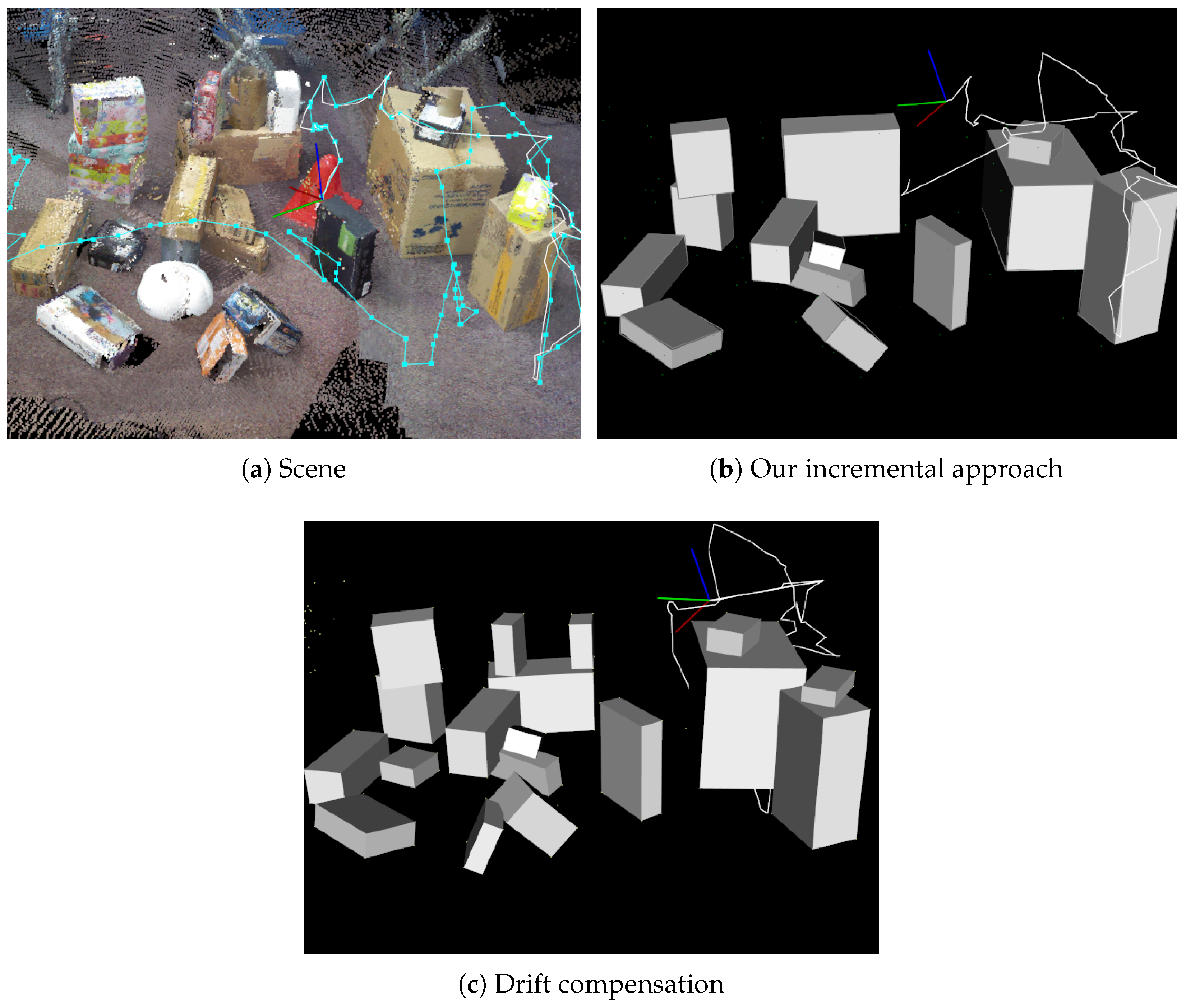
6. Drift Compensation
6.1. Overview
6.2. Cuboid Matching
6.3. Camera Pose Refinement
6.4. Local Plane Map Refinement
7. Interactive Cuboid Modeling
8. Evaluation
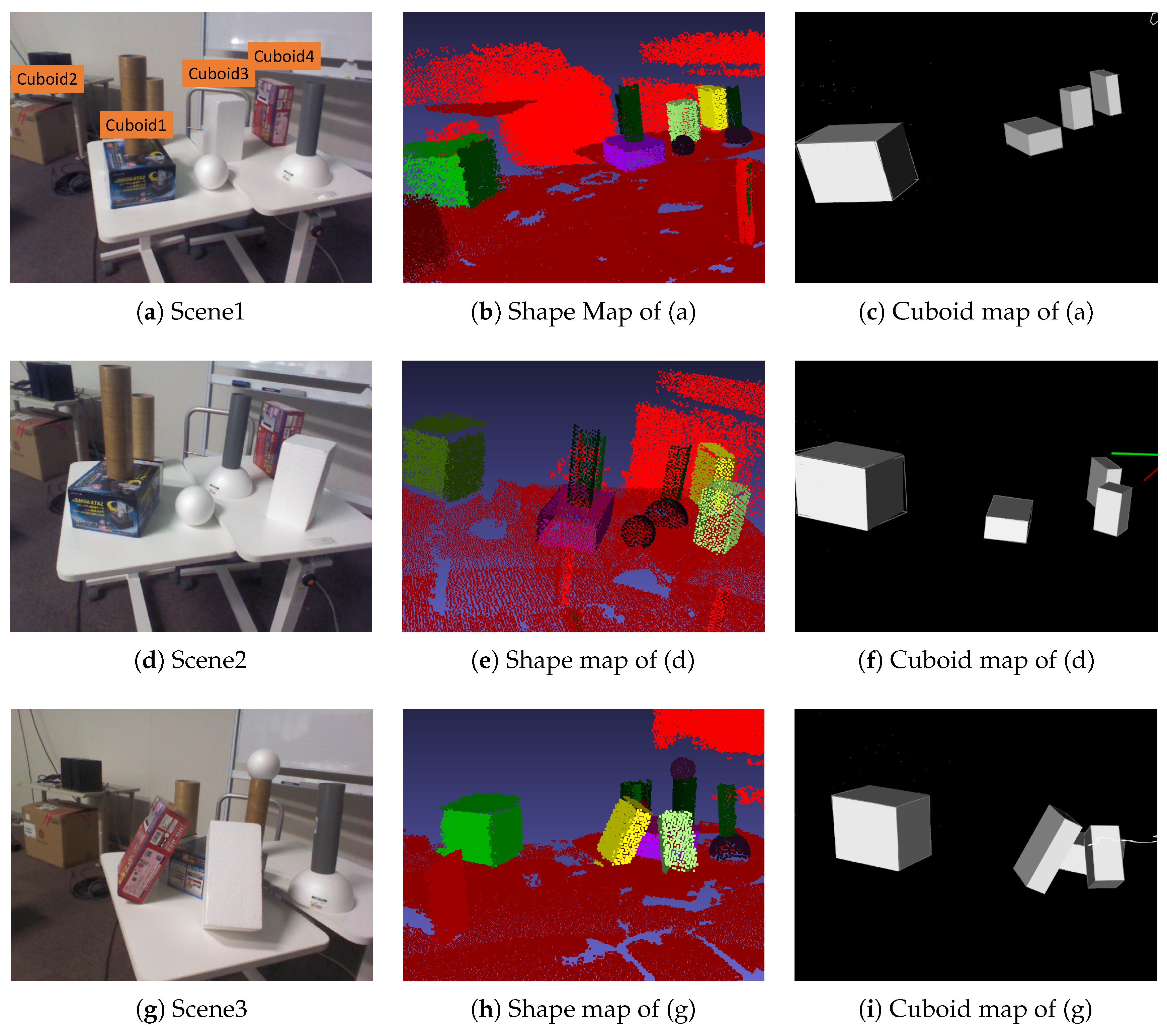
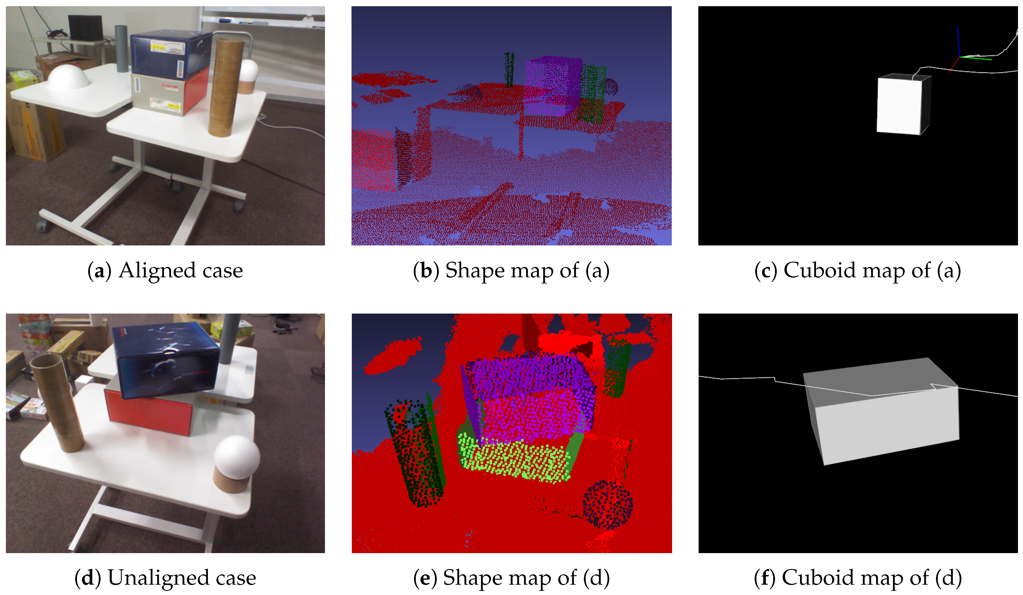
8.1. Cuboid-Shape Estimation
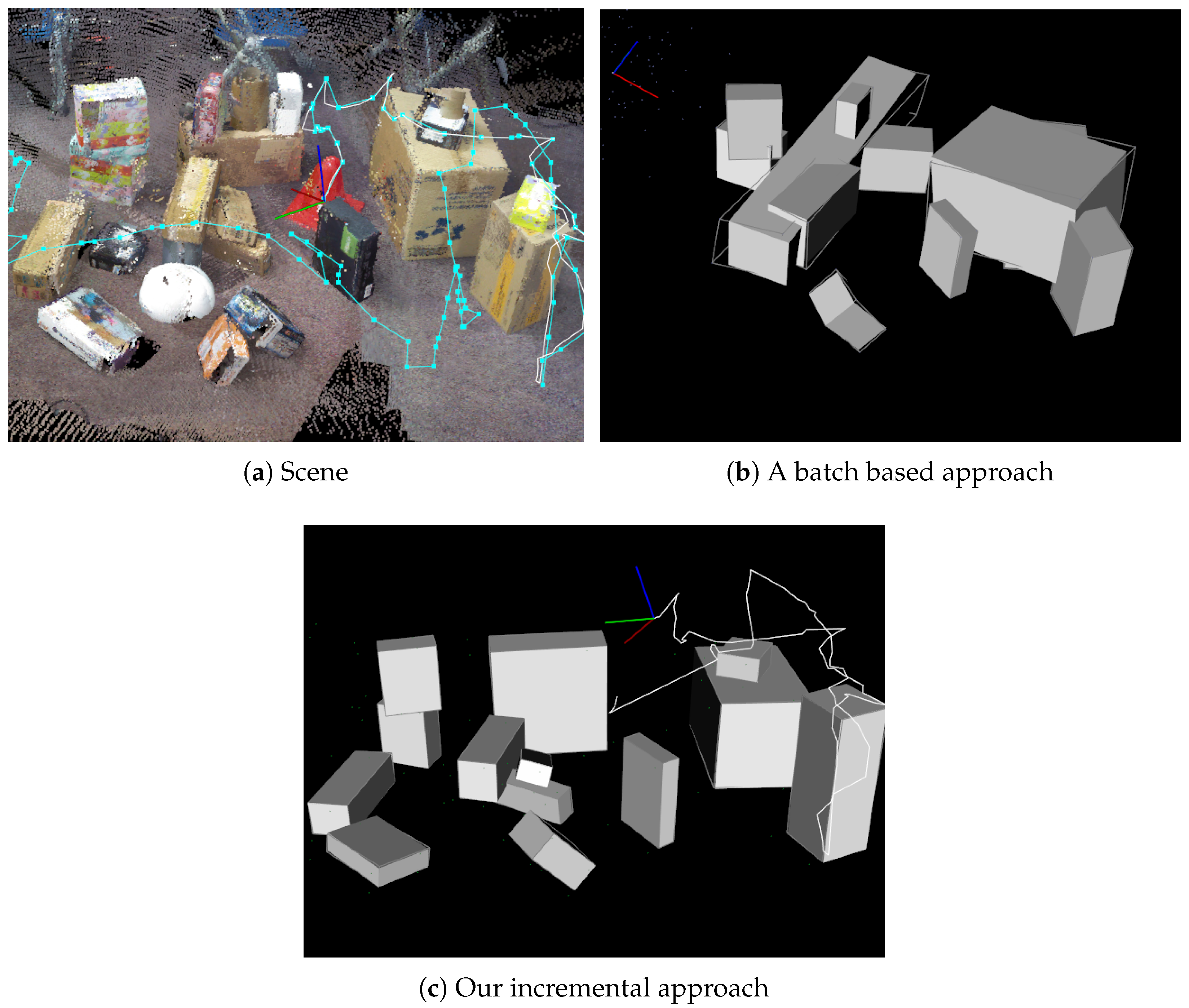
8.2. Cuboid Detection in a Cluttered Environment
8.3. Effectiveness of Drift Compensation
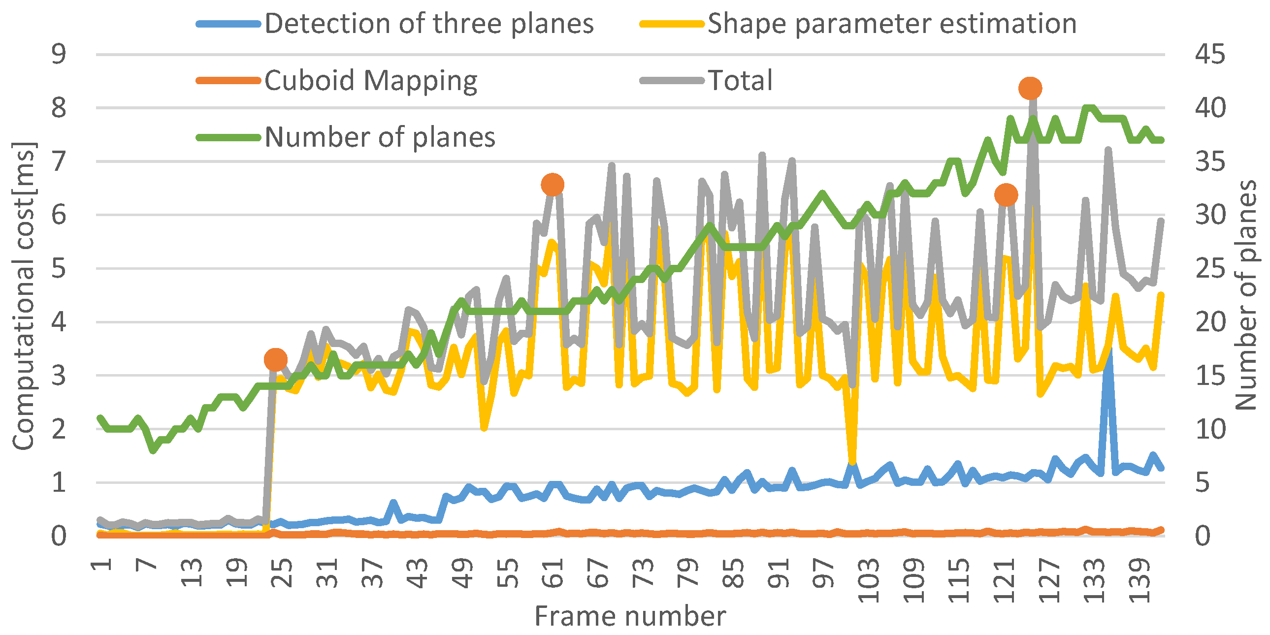
8.4. Computational Cost
8.5. Limitation
9. Conclusions
Author Contributions
Funding
Conflicts of Interest
References
- Saxena, A.; Driemeyer, J.; Ng, A.Y. Robotic grasping of novel objects using vision. Int. J. Robot. Res. 2008, 27, 157–173. [Google Scholar] [CrossRef]
- Hedau, V.; Hoiem, D.; Forsyth, D. Recovering the spatial layout of cluttered rooms. In Proceedings of the IEEE 12th International Conference on Computer Vision, Kyoto, Japan, 29 September–2 October 2009; pp. 1849–1856. [Google Scholar]
- Hedau, V.; Hoiem, D.; Forsyth, D. Thinking inside the box: Using appearance models and context based on room geometry. In European Conference on Computer Vision; Springer: Berlin, Germany, 2010; pp. 224–237. [Google Scholar]
- Del Pero, L.; Guan, J.; Brau, E.; Schlecht, J.; Barnard, K. Sampling bedrooms. In Proceedings of the IEEE Conference on Computer Vision and Pattern Recognition (CVPR), Colorado Springs, CO, USA, 20–25 June 2011; pp. 2009–2016. [Google Scholar]
- Xiao, J.; Russell, B.; Torralba, A. Localizing 3D cuboids in single-view images. In Advances in Neural Information Processing Systems; Curran Associates: Lake Tahoe, NV, USA, 2012; pp. 746–754. [Google Scholar]
- Hejrati, M.; Ramanan, D. Categorizing cubes: Revisiting pose normalization. In Proceedings of the IEEE Winter Conference on Applications of Computer Vision (WACV), Lake Placid, NY, USA, 7–10 March 2016; pp. 1–9. [Google Scholar]
- Osada, R.; Funkhouser, T.; Chazelle, B.; Dobkin, D. Shape distributions. ACM Trans. Graph. (TOG) 2002, 21, 807–832. [Google Scholar] [CrossRef]
- Rusu, R.B.; Marton, Z.C.; Blodow, N.; Dolha, M.; Beetz, M. Towards 3D point cloud based object maps for household environments. Robot. Auton. Syst. 2008, 56, 927–941. [Google Scholar] [CrossRef]
- Lin, D.; Fidler, S.; Urtasun, R. Holistic scene understanding for 3d object detection with rgbd cameras. In Proceedings of the IEEE International Conference on Computer Vision (ICCV), Lake Tahoe, NV, USA, 1–8 December 2013; pp. 1417–1424. [Google Scholar]
- Jiang, H.; Xiao, J. A linear approach to matching cuboids in RGBD images. In Proceedings of the IEEE Conference on Computer Vision and Pattern Recognition (CVPR), Columbus, OH, USA, 23–28 June 2013; pp. 2171–2178. [Google Scholar]
- Khan, S.H.; He, X.; Bannamoun, M.; Sohel, F.; Togneri, R. Separating objects and clutter in indoor scenes. In Proceedings of the IEEE Conference on Computer Vision and Pattern Recognition (CVPR), Boston, MA, USA, 7–12 June 2015; pp. 4603–4611. [Google Scholar]
- Ren, Z.; Sudderth, E.B. Three-dimensional object detection and layout prediction using clouds of oriented gradients. In Proceedings of the IEEE Conference on Computer Vision and Pattern Recognition, Las Vegas, NV, USA, 27–30 June 2016; pp. 1525–1533. [Google Scholar]
- Hashemifar, Z.S.; Lee, K.W.; Napp, N.; Dantu, K. Consistent Cuboid Detection for Semantic Mapping. In Proceedings of the IEEE 11th International Conference on Semantic Computing (ICSC), San Diego, CA, USA, 30 January–1 February 2017; pp. 526–531. [Google Scholar]
- Nguyen, T.; Reitmayr, G.; Schmalstieg, D. Structural modeling from depth images. IEEE Trans. Vis. Comput. Graph. 2015, 21, 1230–1240. [Google Scholar] [CrossRef] [PubMed]
- Balsa-Barreiro, J.; Fritsch, D. Generation of 3D/4D photorealistic building models. The testbed area for 4D Cultural Heritage World Project: The historical center of Calw (Germany). In International Symposium on Visual Computing; Springer: Berlin, Germany, 2015; pp. 361–372. [Google Scholar]
- Balsa-Barreiro, J.; Fritsch, D. Generation of visually aesthetic and detailed 3D models of historical cities by using laser scanning and digital photogrammetry. Digit. Appl. Archaeol. Cult. Herit. 2018, 8, 57–64. [Google Scholar] [CrossRef]
- Reutebuch, S.E.; Andersen, H.E.; McGaughey, R.J. Light detection and ranging (LIDAR): An emerging tool for multiple resource inventory. J. Forest. 2005, 103, 286–292. [Google Scholar]
- Roberto, R.A.; Uchiyama, H.; Lima, J.P.S.; Nagahara, H.; Taniguchi, R.I.; Teichrieb, V. Incremental structural modeling on sparse visual SLAM. IPSJ Trans. Comput. Vis. Appl. 2017, 9, 5. [Google Scholar] [CrossRef]
- Roberto, R.; Lima, J.P.; Uchiyama, H.; Arth, C.; Teichrieb, V.; Taniguchi, R.; Schmalstieg, D. Incremental Structural Modeling Based on Geometric and Statistical Analyses. In Proceedings of the IEEE Winter Conference on Applications of Computer Vision (WACV), Lake Tahoe, NV, USA, 12–15 March 2018; pp. 955–963. [Google Scholar]
- Pradeep, V.; Rhemann, C.; Izadi, S.; Zach, C.; Bleyer, M.; Bathiche, S. MonoFusion: Real-time 3D reconstruction of small scenes with a single web camera. In Proceedings of the IEEE International Symposium on Mixed and Augmented Reality (ISMAR), Adelaide, Australia, 1–4 October 2013; pp. 83–88. [Google Scholar]
- Olivier, N.; Uchiyama, H.; Mishima, M.; Thomas, D.; Taniguchi, R.; Roberto, R.; Lima, J.P.; Teichrieb, V. Live Structural Modeling using RGB-D SLAM. In Proceedings of the 2018 IEEE International Conference on Robotics and Automation (ICRA), Brisbane, Australia, 21–25 May 2018; pp. 6352–6358. [Google Scholar]
- Goldman, R. Intersection of three planes. In Graphics Gems; Academic Press Professional, Inc.: Cambridge, MA, USA, 1990; p. 305. [Google Scholar]
- Mishima, M.; Uchiyama, H.; Thomas, D.; Taniguchi, R.; Roberto, R.; Lima, J.P.; Teichrieb, V. RGB-D SLAM based Incremental Cuboid Modeling. ECCV Workshop 3D Reconstruction in the Wild. 2018. Available online: http://www.sys.info.hiroshima-cu.ac.jp/3drw2018/procs/W17-08.pdf (accessed on 1 January 2019).
- Dwibedi, D.; Malisiewicz, T.; Badrinarayanan, V.; Rabinovich, A. Deep cuboid detection: Beyond 2d bounding boxes. arXiv, 2016; arXiv:1611.10010. [Google Scholar]
- Nguatem, W.; Drauschke, M.; Mayer, H. Finding cuboid-based building models in point clouds. ISPRS Int. Arch. Photogramm. Remote Sens. Spat. Inf. Sci. 2012, XXXIX-B3, 149–154. [Google Scholar] [CrossRef]
- Zhang, C.; Hu, Y. CuFusion: Accurate real-time camera tracking and volumetric scene reconstruction with a cuboid. Sensors 2017, 17, 2260. [Google Scholar] [CrossRef] [PubMed]
- Rodriguez-Garavito, C.; Camacho-Munoz, G.; Álvarez-Martínez, D.; Cardenas, K.V.; Rojas, D.M.; Grimaldos, A. 3D object pose estimation for robotic packing applications. In WEA 2018: Applied Computer Sciences in Engineering; Springer: Berlin, Germany, 2018; pp. 453–463. [Google Scholar]
- Schnabel, R.; Wahl, R.; Klein, R. Efficient RANSAC for point-cloud shape detection. In Computer Graphics Forum; Wiley Online Library: Hoboken, NJ, USA, 2007; Volume 26, pp. 214–226. [Google Scholar]
- Labbé, M.; Michaud, F. Online global loop closure detection for large-scale multi-session graph-based slam. In Proceedings of the IEEE/RSJ International Conference on Intelligent Robots and Systems (IROS 2014), Chicago, IL, USA, 14–18 September 2014; pp. 2661–2666. [Google Scholar]
- Labbe, M.; Michaud, F. Appearance-based loop closure detection for online large-scale and long-term operation. IEEE Trans. Robot. 2013, 29, 734–745. [Google Scholar] [CrossRef]
- Stein, S.C.; Wörgötter, F.; Schoeler, M.; Papon, J.; Kulvicius, T. Convexity based object partitioning for robot applications. In Proceedings of the IEEE International Conference on Robotics and Automation (ICRA), Hong Kong, China, 31 May–7 June 2014; pp. 3213–3220. [Google Scholar]
- Sinha, S.N.; Steedly, D.; Szeliski, R.; Agrawala, M.; Pollefeys, M. Interactive 3D architectural modeling from unordered photo collections. ACM Trans. Graph. (TOG) 2008, 27, 159. [Google Scholar] [CrossRef]
- Shao, T.; Xu, W.; Zhou, K.; Wang, J.; Li, D.; Guo, B. An interactive approach to semantic modeling of indoor scenes with an rgbd camera. ACM Trans. Graph. (TOG) 2012, 31, 136. [Google Scholar] [CrossRef]
- Zhang, Y.; Luo, C.; Liu, J. Walk&sketch: Create floor plans with an rgb-d camera. In Proceedings of the ACM Conference on Ubiquitous Computing; ACM: New York, NY, USA, 2012; pp. 461–470. [Google Scholar]
- Du, H.; Henry, P.; Ren, X.; Cheng, M.; Goldman, D.B.; Seitz, S.M.; Fox, D. Interactive 3D modeling of indoor environments with a consumer depth camera. In Proceedings of the 13th International Conference on Ubiquitous Computing, Beijing, China, 17–21 September 2011; pp. 75–84. [Google Scholar]
- Kim, Y.M.; Mitra, N.J.; Huang, Q.; Guibas, L. Guided Real-Time Scanning of Indoor Objects. In Computer Graphics Forum; Wiley Online Library: Hoboken, NJ, USA, 2013; Volume 32, pp. 177–186. [Google Scholar]
- Newcombe, R.A.; Izadi, S.; Hilliges, O.; Molyneaux, D.; Kim, D.; Davison, A.J.; Kohi, P.; Shotton, J.; Hodges, S.; Fitzgibbon, A. KinectFusion: Real-time dense surface mapping and tracking. In Proceedings of the 10th IEEE International Symposium on Mixed and Augmented Reality (ISMAR), Basel, Switzerland, 26–29 October 2011; pp. 127–136. [Google Scholar]


| Cuboid 1 | Depth | Width | Height | Cuboid 2 | Depth | Width | Height |
| Ground truth | 16.0 | 22.5 | 10.5 | Ground truth | 46.6 | 49.8 | 41.0 |
| Scene 1 | 16.8 | 23.5 | 9.8 | Scene1 | 46.9 | 50.3 | 34.1 |
| Scene 2 | 16.8 | 23.1 | 9.6 | Scene2 | 40.9 | 50.7 | 36.5 |
| Scene 3 | 16.3 | 24.6 | 9.8 | Scene3 | 39.8 | 47.1 | 31.2 |
| Cuboid 3 | Depth | Width | Height | Cuboid 4 | Depth | Width | Height |
| Ground truth | 9.8 | 9.8 | 19.7 | Ground truth | 7.9 | 16.0 | 21.8 |
| Scene 1 | 10.3 | 10.7 | 19.2 | Scene 1 | 7.0 | 17.2 | 21.3 |
| Scene 2 | 10.7 | 11.4 | 19.4 | Scene 2 | 7.4 | 19.4 | 21.9 |
| Scene 3 | 9.9 | 10.5 | 19.3 | Scene 3 | 7.2 | 16.7 | 21.2 |
| Batch | Ours | |
|---|---|---|
| Precision | 0.64 | 0.92 |
| Recall | 0.37 | 0.63 |
| Batch | Positive | Negative |
| True | 7 | - |
| False | 4 | 12 |
| Ours | Positive | Negative |
| True | 12 | - |
| False | 1 | 7 |
| Incremental | Drift Compensation | |
|---|---|---|
| Precision | 0.92 | 0.94 |
| Recall | 0.63 | 0.89 |
| Incremental | Positive | Negative |
| True | 12 | - |
| False | 1 | 7 |
| Drift compensation | Positive | Negative |
| True | 17 | - |
| False | 1 | 2 |
© 2019 by the authors. Licensee MDPI, Basel, Switzerland. This article is an open access article distributed under the terms and conditions of the Creative Commons Attribution (CC BY) license (http://creativecommons.org/licenses/by/4.0/).
Share and Cite
Mishima, M.; Uchiyama, H.; Thomas, D.; Taniguchi, R.-i.; Roberto, R.; Lima, J.P.; Teichrieb, V. Incremental 3D Cuboid Modeling with Drift Compensation. Sensors 2019, 19, 178. https://doi.org/10.3390/s19010178
Mishima M, Uchiyama H, Thomas D, Taniguchi R-i, Roberto R, Lima JP, Teichrieb V. Incremental 3D Cuboid Modeling with Drift Compensation. Sensors. 2019; 19(1):178. https://doi.org/10.3390/s19010178
Chicago/Turabian StyleMishima, Masashi, Hideaki Uchiyama, Diego Thomas, Rin-ichiro Taniguchi, Rafael Roberto, João Paulo Lima, and Veronica Teichrieb. 2019. "Incremental 3D Cuboid Modeling with Drift Compensation" Sensors 19, no. 1: 178. https://doi.org/10.3390/s19010178
APA StyleMishima, M., Uchiyama, H., Thomas, D., Taniguchi, R.-i., Roberto, R., Lima, J. P., & Teichrieb, V. (2019). Incremental 3D Cuboid Modeling with Drift Compensation. Sensors, 19(1), 178. https://doi.org/10.3390/s19010178