1. Introduction
Automatic people detection in video sequences is one of the most relevant problems in computer vision, which is essential in many applications such as for video-surveillance, human–computer interaction and mobile robotics. Although generic object detection is maturing very rapidly thanks to the recent widespread use of deep learning [
1,
2], many challenges still exist for the specific case of detecting people. Video and images of people exhibit a great variation of viewpoints, motion, poses, backgrounds, occlusions, sizes and body-part deformations [
3]. Detection performance has a strong dependency on the training data used to build detectors [
4] and, therefore, accuracy drops are expected when training and testing data have different patterns [
5]. Moreover, people detectors often have many parameters, which are heuristically or experimentally set according to training data. Such parameter setting strategy may have limitations when applied to other data different from the training one.
The adaptation of people detectors is therefore desired to successfully apply such detectors to unseen data [
6]. This adaptation can be approached as best algorithm selection [
7,
8], domain adaptation for learning scene-specific detectors [
9], data augmentation for the video-surveillance domain [
10] and unsupervised feature learning [
3,
4]. However, these approaches imply retraining models for the new target domain, which may not be possible in certain applications such as real-time video-surveillance where data may not be available in advance. Alternatively, one may adapt detectors for testing time without changing any model by combining multiple features [
11], embedding detection within a multi-class Bayesian classification [
5], designing cascades of heterogeneous detectors [
12] or coupling detection and tracking [
13,
14]. However, these approaches impose restrictions on the employed detectors (e.g., high precision and low recall [
14]) or require the use of tracking [
13,
14].
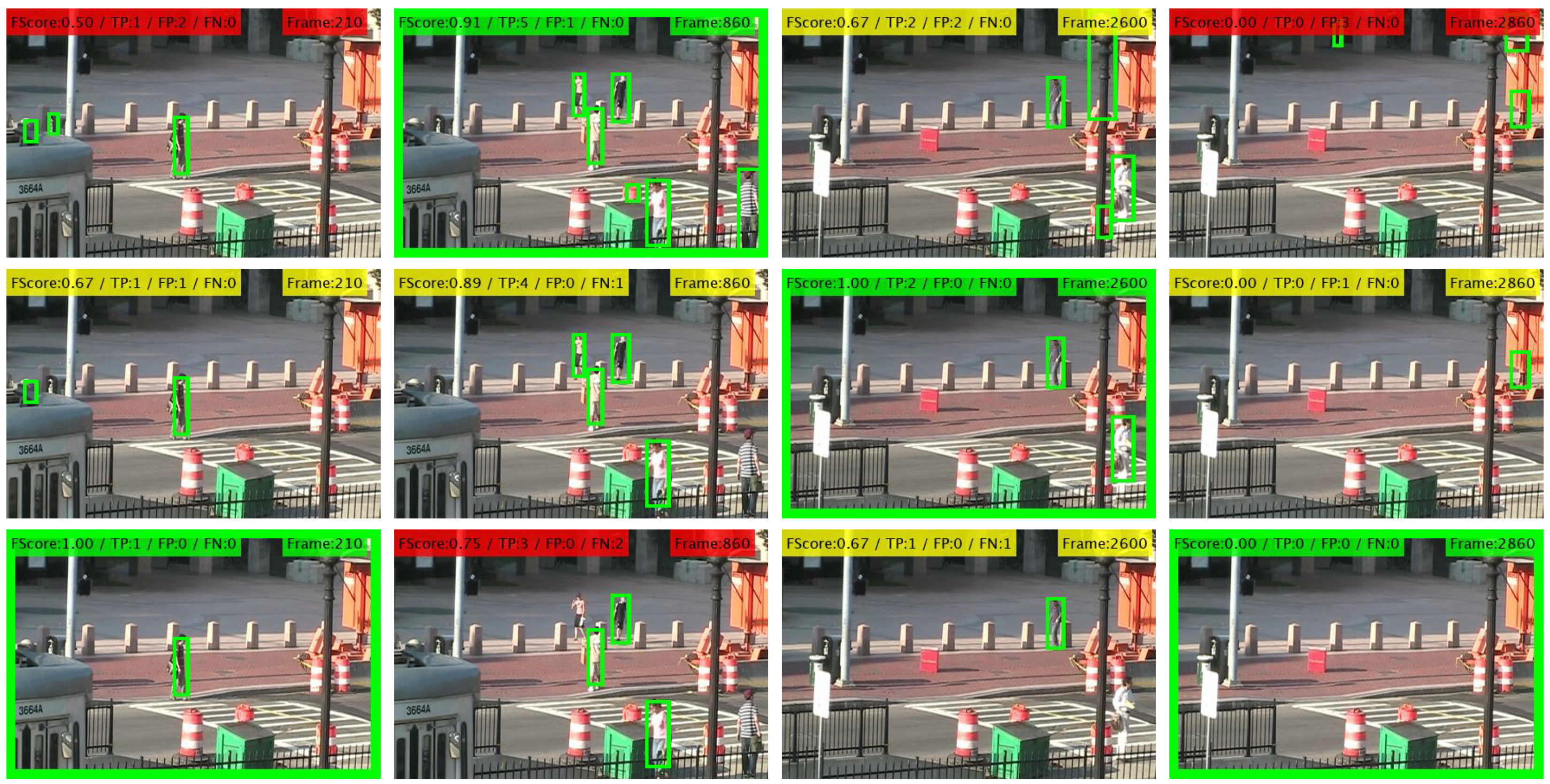
To overcome the above-mentioned shortcomings, in this paper, we propose a coarse-to-fine framework to adapt the configuration of people detectors during testing time. In particular, we focus on the thresholding stage that determines the detector output (i.e., bounding boxes), being quite popular among a wide variety of recent detectors and having a strong impact on detector’s performance (see examples in
Figure 1). We employ multiple detectors to simultaneously find their optimal threshold values within an optimization framework based on their mutual information [
15]. Our proposal explores multiple thresholding hypotheses for all employed detectors and exploits pair-wise correlations between their outputs within a coarse-to-fine adaptation strategy. First, a coarse stage employs correlation entropy to identify which frames of the video sequence contain people and therefore enables speeding up the detection process by avoiding analyzing frames without people. Second, a fine adaptation stage is performed for frames where people are present by optimally selecting the detection threshold for each detector. Such selection is performed for each detector by accumulating all pair-wise comparisons with other detectors. Finally, we obtain the output of each detector by applying the obtained threshold value. The proposed framework only requires threshold-based detectors with an output in the form of bounding boxes. Therefore, it can be applied to many recent approaches, as demonstrated by the experimental results, which show that adapting sets of people detectors (from two to six) outperforms individual detectors tuned to obtain maximum performance (i.e., whose threshold is trained offline and fixed in advance). Preliminary results are published in [
15].
The remainder of the paper is structured as follows.
Section 2 describes the related work.
Section 3 describes the proposed coarse-to-fine adaptation framework based on cross-correlations.
Section 4 presents the experiments. Finally,
Section 5 concludes this paper.
2. State of the Art
Adapting pedestrian detectors to specific scenes is frequently termed as
domain adaptation where the original training dataset (i.e.,
source domain) is fully annotated. Existing approaches adapt such detectors to unseen data (i.e.,
target domain) which can be focused on features or models [
16].
Feature-based approaches aim to transform feature spaces between the source and target domains, and then apply a classifier. Early approaches annotate data in the target domain to define a grid classifier from scratch [
17]. Albeit effective, such annotation is time-demanding, several data samples are needed and therefore difficult to perform for other domains. Most of recent feature-based approaches focus on
transfer learning where the knowledge from source domains is extended to semantically-similar categories of the target domain by retraining models with few data annotations. Transfer-learning can use bounding boxes from both the source and target domain such as the learning of discriminative models using CNNs and data augmentation [
10] and the transfer of shared source-target attributes by feature selection where data distributions of the domains are similar [
18]. Moreover, approaches can also assume the absence of annotations for the target domain and, therefore, perform an online self-learning process by determining which samples to select. For example, such selection can use super-pixel region clustering [
19], Gaussian regression within a hierarchical adaptive SVM [
16], confidence scores within a deep model [
3], background modeling [
20] and multiple contextual cues [
4]. Other strategies may also be applied by weighting the source data to match the distribution of the object categories in the target domain before re-training [
4], by propagating labels between frames for good positive instances [
20] and by integrating classifiers at image and instance level to maintain semantic consistency between two domains [
21]. Image level aims to determine whether source or target domains are analyzed, whereas instance level classifier is focused on the feature maps. Finally, transfer learning using synthetic data has recently been proposed [
22,
23]. However, training complex models still presents challenges due to the visual mismatch with real data [
20].
Model-based approaches focus on adapting the parameters of the classifiers or the strategy applied. For example, in [
5], a Bayes-based multi-class classifier is adapted by computing the proportion of objects in the target domain during runtime. Such adaptation may focus on correcting detection errors by spatiotemporal filtering [
24]. Other approaches make
use of context such as for building a partial belief about the current scene to only execute certain classifiers [
25], for applying specific combinations of part-based models based on spatial object information [
26] and for modulating object proposals (class prior probabilities) with semantic knowledge [
27]. Model-based approaches may also combine different models by learning the weights of predictions for different sensor modalities in an online manner [
11], by applying a cascade of detectors designed to combine the confidence of heterogeneous detectors [
12], and by selecting automatically the most suitable model for visible or non-visible light images [
28]. Another approach focuses on automatically learning classifiers on the target domain without annotated data, which are later evaluated in the source domain with labeled data and finally top-performing classifiers are selected as the most reliable for the target domain [
29]. Moreover, model-based approaches may perform
detector ranking by estimating the similarity between both domains in some feature space to design a cost function for selecting the best algorithm in each situation or domain [
7]. Therefore, detector ranking can be efficiently learned for different target domain subsets [
8] but requires full annotation of source and target domain. Similar to feature-based approaches, model-based detector adaptation may be achieved by
coupling detection and tracking for online retraining single [
13] or multiple [
14] detectors without annotated data. However, these approaches share the limitations of transfer learning (detector re-training), impose restrictions on the employed detectors (e.g., high precision and low recall [
14]) or require the use of tracking which is may lead to unstable results [
13,
14].
Table 1 compares the proposed and reviewed approaches. As we can observe, the proposed approach avoids re-training detectors, unlike many model-based and feature-based approaches based on transfer learning, which often require an offline training stage before the final application to the target domain. Instead of selecting accurate samples for re-training, we leverage results from multiple and possibly independent people detectors assuming that their errors are diverse. The detection threshold of each detector is adjusted according to similarities to other employed detectors. Moreover, our proposal applies self-learning in an online fashion without requiring annotated data for the target domain, unlike those in [
26,
27] and also without requiring a prior analysis of the target domain features [
7,
8]. Additionally, the proposed approach employs standard outputs of people detectors (i.e., bounding boxes) so it can be applied to a wide variety of existing approaches, unlike other approaches restricted to CNNs [
10], Faster R-CNN [
21], and SVMs [
16,
18] or to being coupled with other detectors [
11] and trackers [
13]. Finally, the proposed approach is applied to video sequences, unlike most of those in the literature, which are focused on image-level classification. Such application to video may determine when and where adaptation might improve performance, and therefore adjust the computational complexity to the particular details of each video sequence.
3. Detector Adaptation Framework
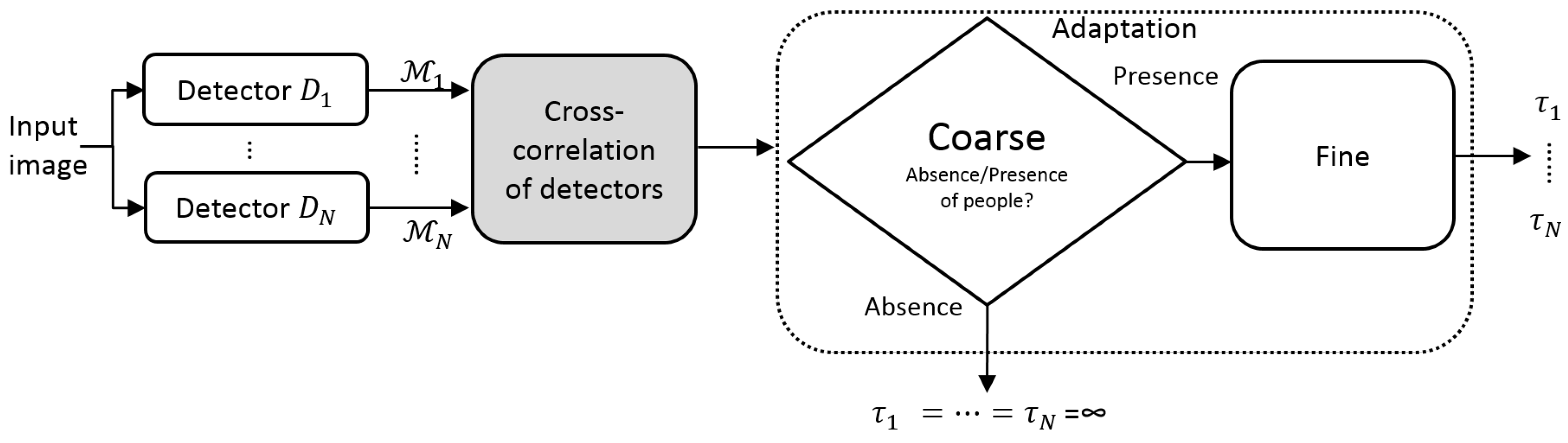
We propose a coarse-to-fine framework to improve detector’s performance at runtime classification by adapting the configuration of each detector employed (see
Figure 2). This proposal is inspired by the
maximization of mutual information strategy where classifiers are combined assuming that their errors are complementary, being successfully applied for example to detect shadows [
30] and skin [
31]. We extend such maximization framework to people detection by introducing pair-wise detector correlation and by adapting online their configuration. Note that we are not re-training detectors at prediction time, which may require data not available in real applications or highly-accurate detectors, and may imply high latency [
5], i.e., a minimum number of frames to compute accurate decisions over time. Instead, we consider generic threshold-based detectors pre-trained on standard datasets, thus making this proposal applicable to a wide variety of detectors.
Assuming a set of
N people detectors
applied to an image, each detector
obtains a confidence map
describing the people likelihood for each spatial location (
) and scale
s in the image. Then, detection candidates are obtained by thresholding this map:
where
and
is the detection threshold whose value is heuristically set based on the confidence map. These candidates are later combined across scales and can be post-processed by a variety of techniques such as non-maximum suppression [
32] and background-people segmentation [
33]. The final result for each detector is a set
with
detections (i.e., bounding boxes) representing the output of the detector
where each detection
(i.e., bounding box) is described by its position (
) and dimensions (
). A key parameter in this procedure is the detection threshold
, which determines the number of detection candidates. Low (high) values of
generate several (few) detections increasing the false (true) positive rate: three examples of
are shown in
Figure 1. We propose to adapt such detection threshold to the image context by exploring similarities with the other detectors.
We compare the output of detectors to obtain a set of pair-wise correlation scores (
cross-correlation of detectors in
Figure 2), which measures the output similarity. This stage is extended in
Section 3.1.
We analyze this similarity at two different levels. First, we propose a coarse analysis to determine relevant frames in a video sequence, where people are present. Second, a fine analysis is applied in those selected frames to adapt the detection system, i.e., adjust the detection thresholds.
3.1. Cross-Correlation of Detectors
Firstly, we explore the decision space to determine each detector output by applying multiple thresholds. Then, we correlate these multiple outputs for each pair of detectors (
and
) to obtain a correlation map
which measures the output similarity (see
Figure 3).
3.1.1. Multiple Thresholding
To explore the possible detector outputs, we define a set of
L thresholds
for each detector
whose values are determined by considering
L levels between the extreme values of the confidence map
(i.e., minimum and maximum). Then, we perform thresholding with multiple values
to obtain a set of outputs as follows:
where each output
is obtained by applying the threshold
to Equation (1). Note that each detector
may have different threshold values
adapted to the range of values in
.
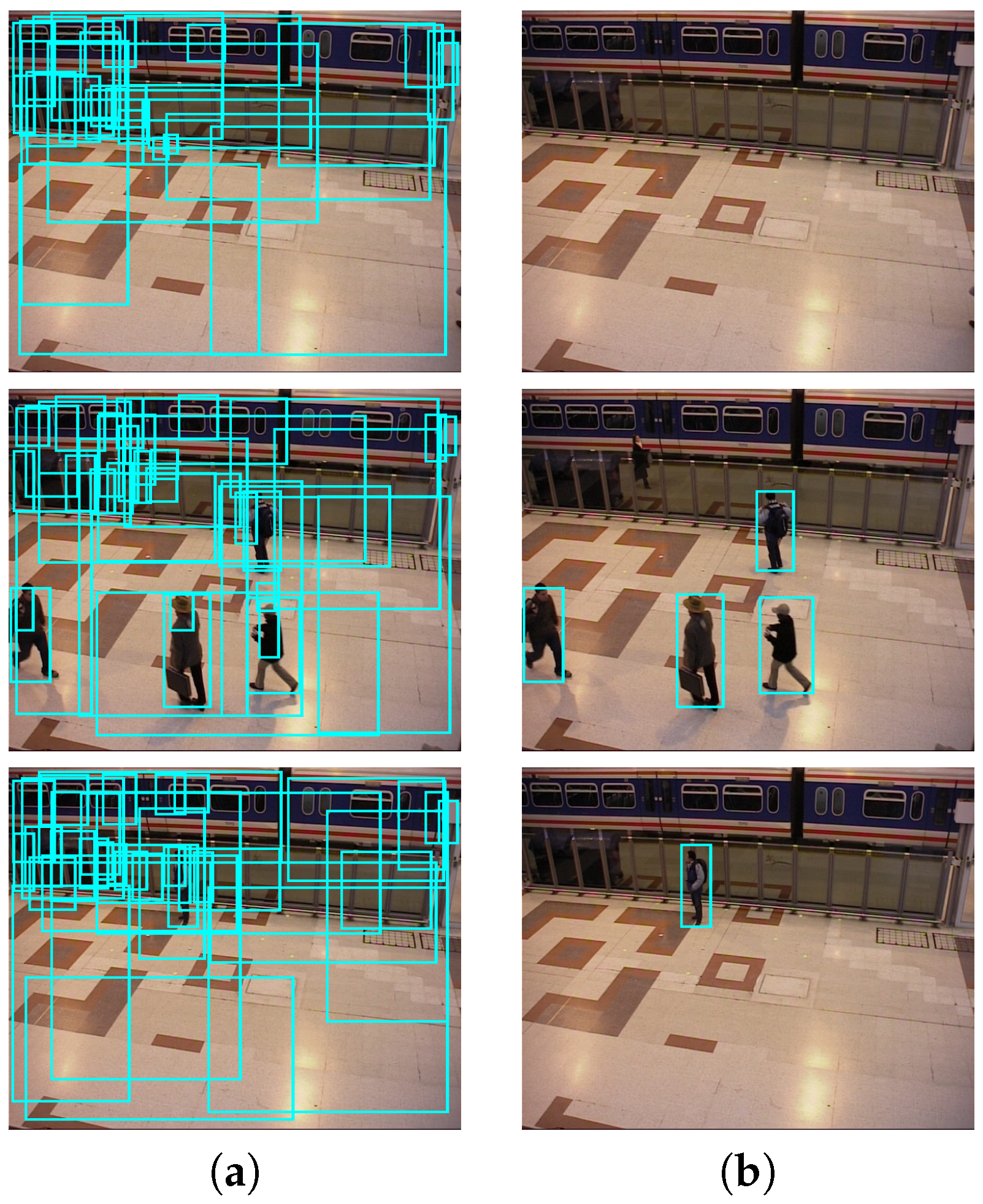
Figure 4 shows three examples (rows) of the possible detector outputs
obtained by applying two different thresholds
and
from the full set
.
3.1.2. Pair-Wise Correlation
We correlate the
N detector outputs
to estimate their similarity. We compute a correlation map
for each pair of detectors outputs
and
. Each element is defined as:
where
is a function to compute the similarity between the output of detectors. The number of correlation maps
to be computed for N detectors is
.
We propose computing
as a one-class classification problem by applying standard evaluation measures. To compare bounding boxes from two outputs, we use three matching criteria [
34]: relative distance
(where
is the image diagonal divided by each
size), cover
and spatial overlap
. The criterion
measures the distance between the bounding box centers of
and
in relation to the size of the bounding boxes in
. Similar to
, criteria
and
employ, respectively, the percentage of spatial bounding box coverage in
and the intersection-over-union features. A positive match is considered true if
,
and
, as commonly employed in related works [
34], which corresponds to a deviation up to 25% of the true object size. Only one
is accepted as correct by matching
(i.e., true positive), so any additional
on the same bounding box is considered as a false positive. Then, we compute precision and recall measures from the matching results and obtain the FScore as the final similarity measure
between
and
as in [
35].
Thus, the final correlation map
between two detectors is defined as the FScores
F:
where
.
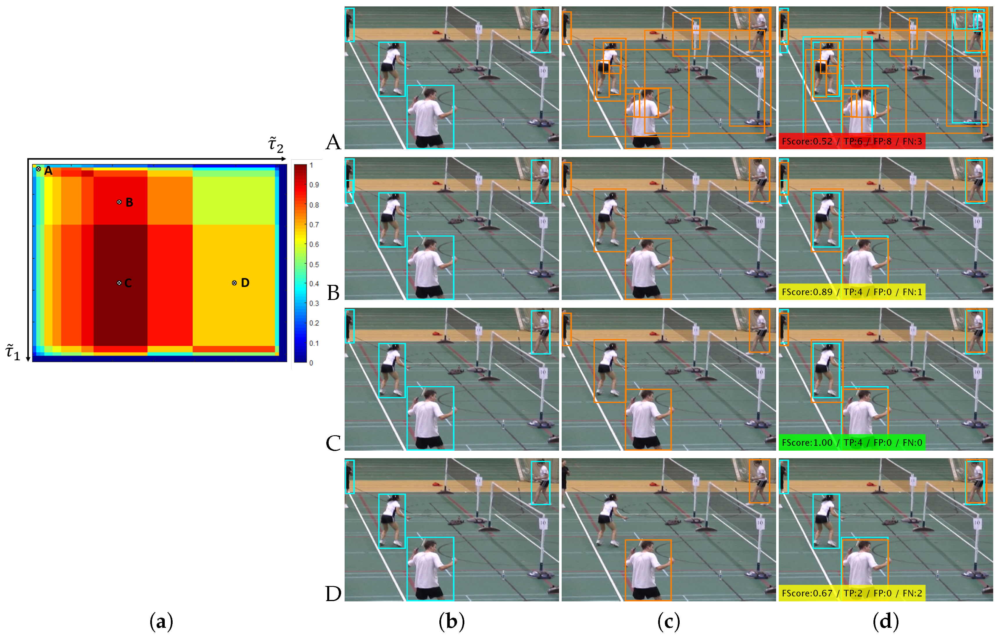
Figure 5 shows one example of correlation map
and four different outputs between two the detectors
(rows A, B, C and D). Example A corresponds to a low threshold value for both detectors (
and
) and therefore in this case a low FScore similarity
. On the other hand, Example C corresponds to a medium-high threshold value for the first detector
and a low-medium threshold value for the second detector
, and therefore in this case a high FScore similarity
.
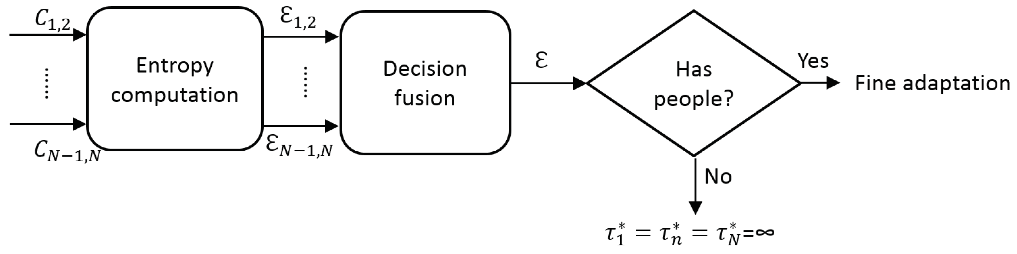
3.2. Coarse Adaptation
Assuming that frames without people are not relevant for the adaptation process, we propose to use the correlation map
to determine the relevant frames in a video sequence. In particular, we propose to measure the information entropy as an estimation of the presence of people in every frame (see
Figure 6).
Based on the principle of maximization of mutual information, we assume that two independent detectors, albeit designed for the same purpose (to detect persons), in presence of people would be highly correlated when many bounding boxes are matched and, therefore, a high level true positive detections is expected. On the other hand, low correlation values would have few matches and, therefore, imply an increase in the false positive rate or negative detection rate. Note that there is one exception to this assumption when outputs are empty (i.e., ) since both outputs are equal and we cannot compute the FScore. To consider this, we avoid this situation by setting the FScore to zero when these sets are empty. However, two independent detectors applied to a frame without the presence of people would have low correlation values for every possible configuration . For that reason, we can assume that those frames with the presence of persons will produce more variable correlation maps than those without people.
We propose estimating the absence/presence of people using the entropy of the correlation map
. Information entropy is defined as the average amount of information produced by a stochastic source of data. The measure of information entropy associated with each possible data value is the negative logarithm of the probability mass function for the value. Entropy is a statistical measure of randomness that can be used to characterize the texture of an input image. In our case, we propose classifying every frame using the entropy over the correlation map
as:
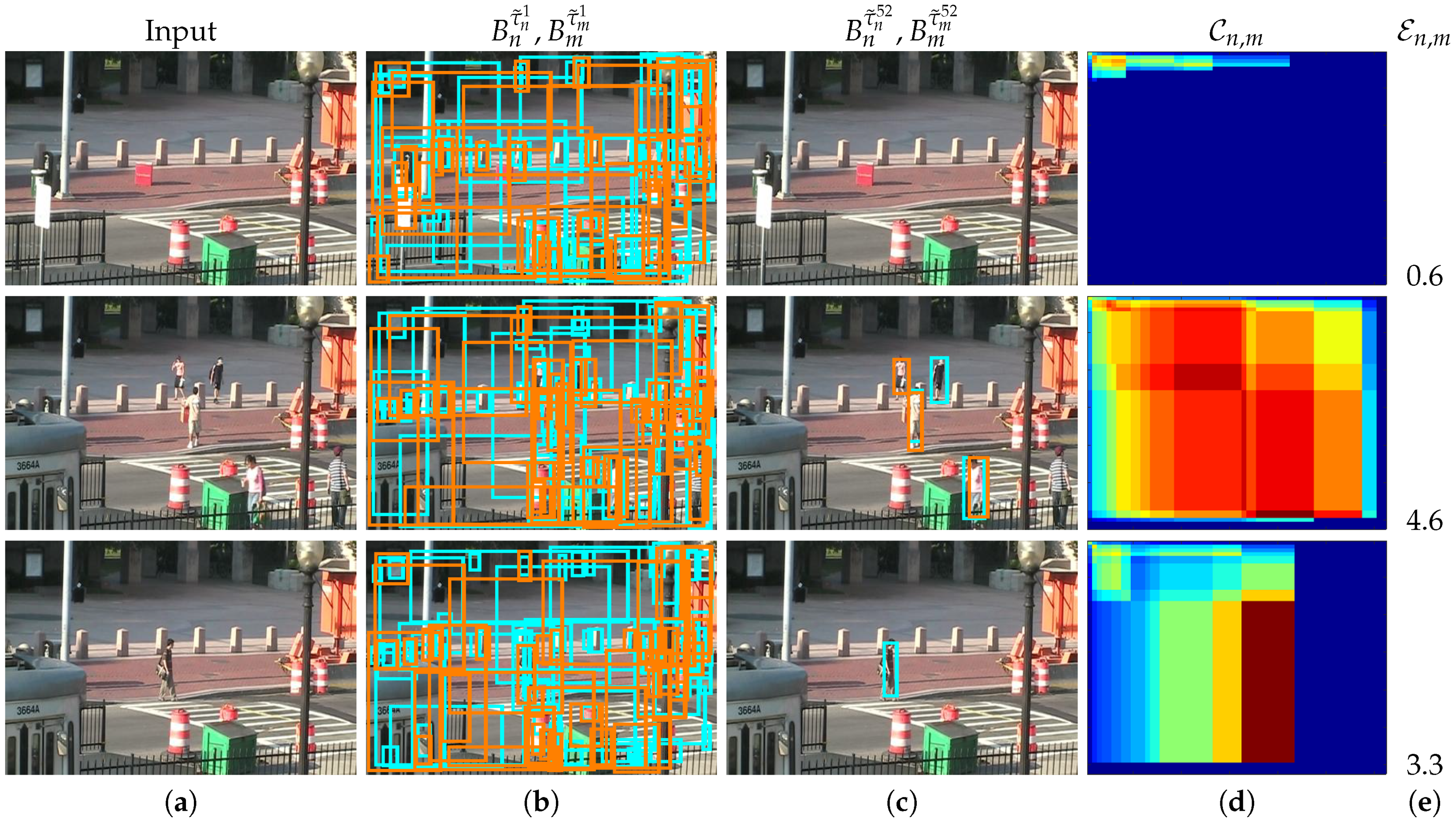
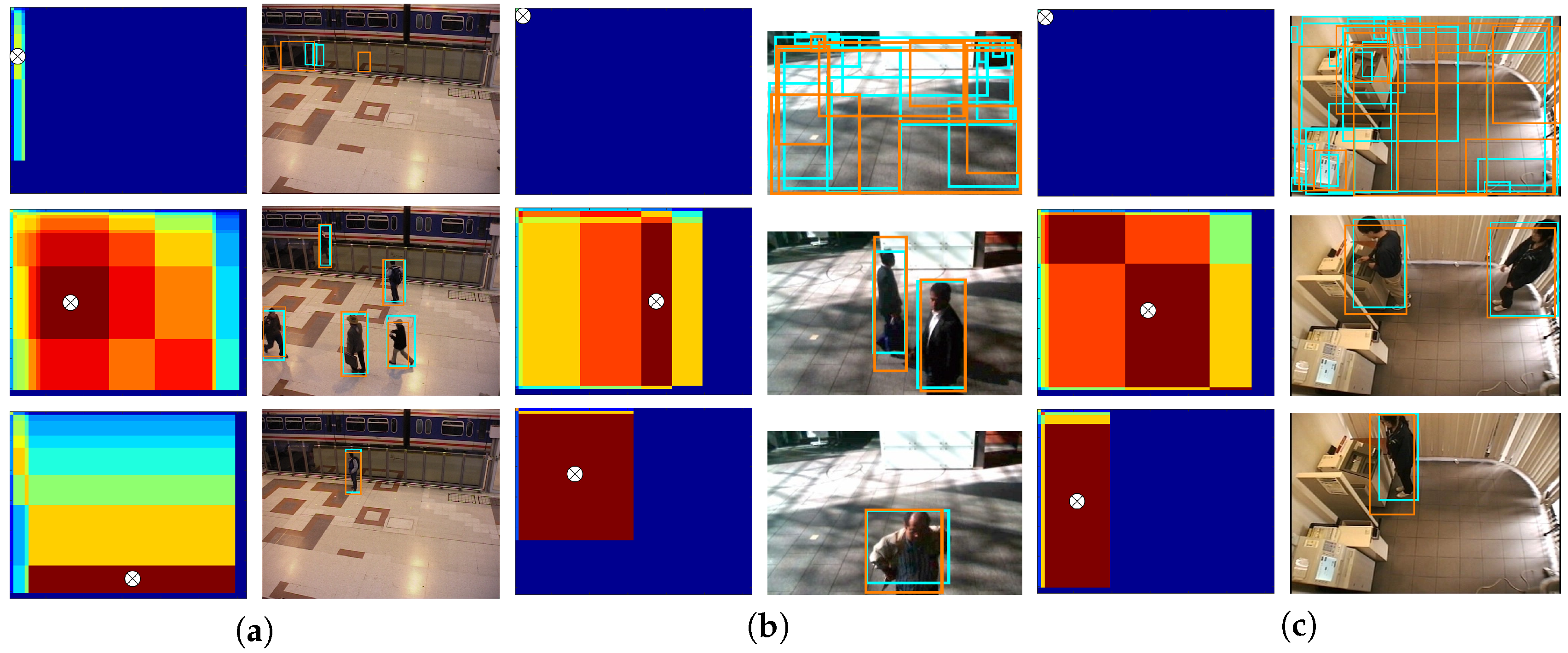
Figure 7 shows three different examples (rows) of correlation maps
, the output of two detectors for two different threshold values (low and high thresholds) and the corresponding entropy
values. Note the three different correlation behaviors: the first example shows an empty scene, almost zero FScore similarity for any possible pair-wise correlation and therefore a low entropy value (
); the second example shows an scene with five pedestrians, high FScore similarity for a range of pair-wise correlations and therefore a high entropy value (
); and the third example shows only one person, a medium-high FScore similarity for a range of pair-wise correlations and therefore a medium-high entropy value (
).
Up to this point, we have a set of hypothesis for presence of people obtained for each compared pair of detectors
(i.e.,
and
), which are combined to obtain a final decision (
decision fusion in
Figure 6). Such hypotheses combination is performed as a traditional mixture of experts via weighted voting [
36]:
where
is the weight for the hypothesis
achieved by comparing
and
and
. Although such ensemble voting may benefit from a previous learning stage [
37], currently we assume no prior knowledge about detectors performance so we consider equal weighting
.
In the case of absence of people (i.e., low value of
), we assume the detections outputs are empty (i.e.,
) and therefore the final configuration for each detector is
. This decision has the potential benefit of avoiding any possible false detection but also the possible disadvantage of losing any correct detections (see visual examples in
Figure 1). On the other side, in the case of presence of people (i.e., high value of
), a further adaptation process is required, therefore it is necessary to analyze the fine similarity for the adaptation process.
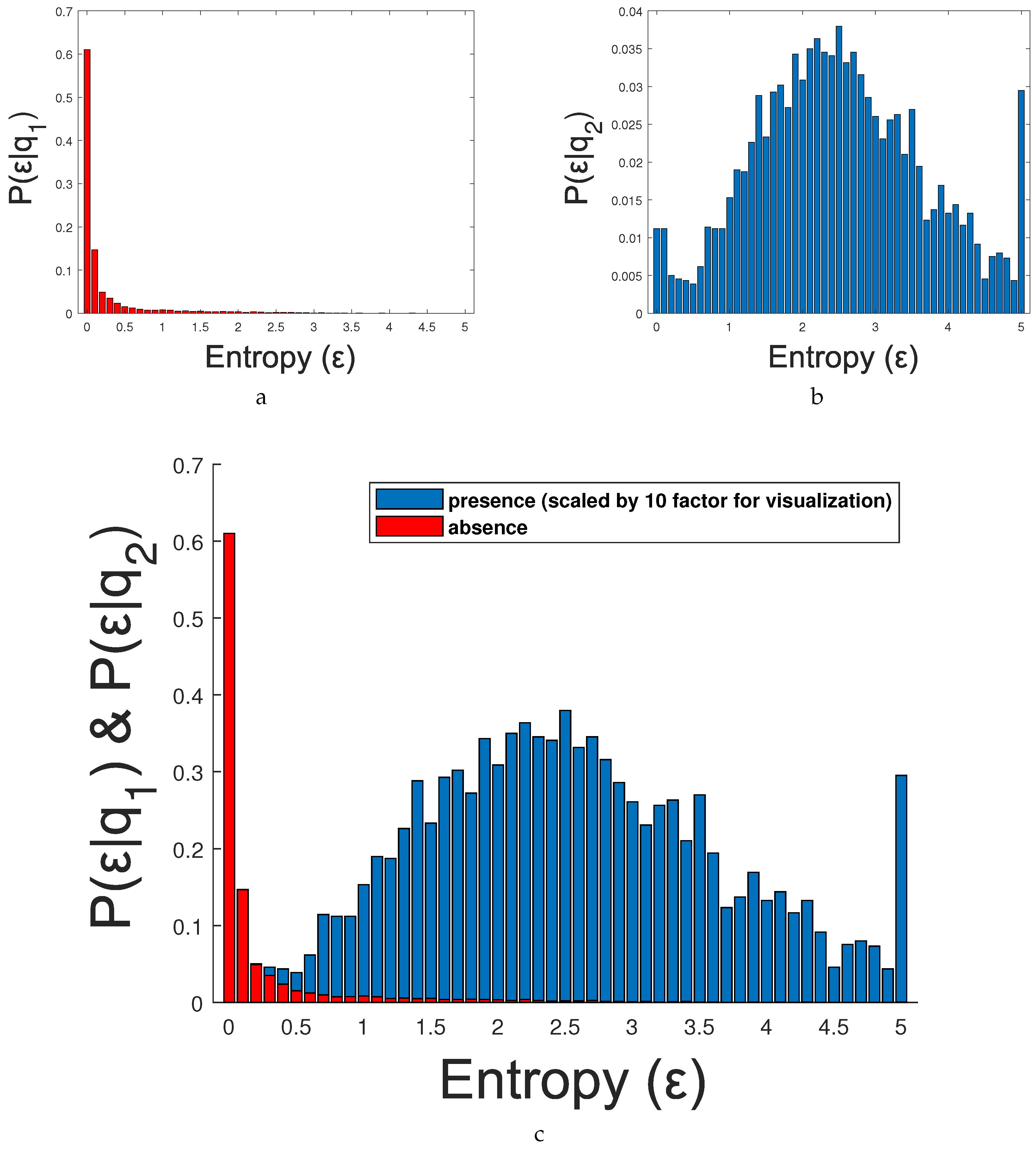
We formulate the detection of frames containing people (i.e., coarse adaptation) as a two-class classification problem where class
indicates the absence of people in a frame and
is the opposite class. We classify the frame based on the evidence provided by the entropy
, we evaluate the posterior probability of each class
and we choose the class with largest
, i.e.,
Then, applying the Bayes Rule results in:
does not affect the decision rule so it can be eliminated. We simplify to the likelihood ratio
:
Finally, assuming equal priors (absence/presence of people), the decision rule is known as the Likelihood Ratio Test (LRT):
which in essence turns into finding the first entropy value
that determines the condition
and using such value as a threshold for the entropy.
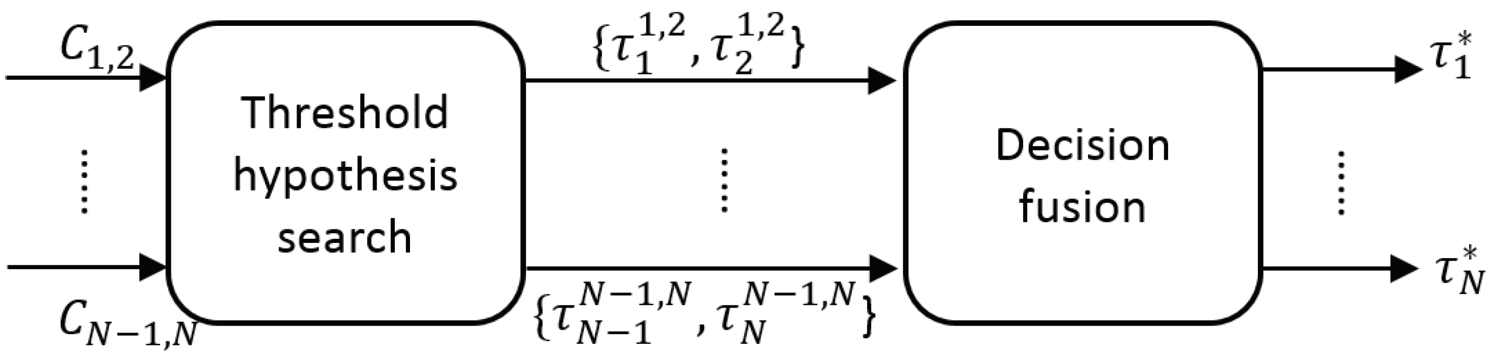
3.3. Fine Adaptation
The aim of the fine adaptation is to find the configuration with the highest similarity (i.e., highest value in
) to select the best detection threshold for each detector (
and
, respectively). The threshold hypothesis selection requires searching a single maximum value in
, which may contain multiple local maxima. The correlation map
is the similarity
between the output of each pair of detectors
and
, and the threshold hypothesis selection can derived as:
where
is defined as Equation (3).
Our problem for finding the optimal global solution can be formulated by following the Maximum Likelihood Estimation (MLE) criterion once computed
:
To find such maximum value, we propose using a sub-optimal global search solution of the threshold hypothesis selection problem with lower computational cost requirements, i.e. Simulated Annealing (SA) [
38]. SA is a probabilistic technique for approximating the global optimum of a given function. For problems where finding an approximate global optimum is more important than finding a precise local optimum in a fixed amount of time, SA may be preferable to other iterative alternatives such as gradient descent [
39].
Moreover, we may assume that the probability of selecting a pair of thresholds (i.e., choosing a specific configuration) depends on the pair of detectors compared. For example, some detectors may tend to use thresholds with low values, whereas other detectors may use high values. Therefore, we include a function
to model the prior distribution of thresholds which determines the most likely pairs of thresholds given two detectors. It can be defined as follows:
Since the solution of Equation (11) or Equation (12) may not be unique, we may obtain various maximum values
(see the darkest area in the bottom-left image in
Figure 5a) as the detectors are never totally independent. Therefore, we currently propose three alternatives: selecting the mean, minimum or maximum value among those thresholds
maximizing
.
After finding the best detection thresholds obtained for each compared pair of detectors
(i.e.,
and
), we combine them to obtain a final configuration for each detector (
decision fusion in
Figure 8).
Such hypotheses combination is performed as in Equation (6) as a traditional mixture of experts via weighted voting as follows:
It is important to note that this equation does not combined people detectors, instead the proposed approach focuses on improving independently each detector by adapting the detection threshold.
5. Conclusions
We have presented a coarse-to-fine framework to automatically adapt people detectors during runtime classification. This proposal explores multiple thresholding hypotheses and exploits the correlation among pairs of detector outputs to determine the best configuration. The coarse adaptation determines the presence/absence of people in every frame and therefore the necessity/not necessity of adaptation of the system. The fine adaptation obtains the optimal detection threshold for each detector in every frame. The proposed approach uses standard state-of-the-art detector outputs (bounding boxes), therefore it can employ various types of detectors. This framework allows the automatic threshold adaptation without requiring a re-training process and therefore without requiring any additional manually labeled ground truth apart from the offline training of the detection model.
The proposed coarse adaptation is able to classify with around 80% of precision and recall both classes absence and presence of people. The fine adaptation results (both MLE and MAP versions) demonstrate that any correlation up to six detectors outperforms state-of-the-art detectors, whose thresholds are optimally trained in advance. In addition, we also explored other sub-optimal threshold hypothesis selection approaches with lower computational cost requirements (number of pair-wise correlations between detectors per frame). In particular, the SA search obtains almost the exhaustive FScore results but with a drastic computational cost reduction. Overall, the final coarse-to-fine framework also outperforms state-of-the-art detectors, for both frame by frame and video analysis results, with a computational cost reduction of around 50%.
For future work, we will study other threshold selection and fusion alternatives and we will apply this proposal to other detectors and object types. We will also explore other additional configurations and not only the detection threshold, for example the position of the bonding box, scale of the detected objects, pose, etc.
We acknowledge that running six detectors significantly increases the required resources as compared to running a single detector. However, this adaptation scheme may not need to be applied for each frame of a video sequence and it may be used periodically (e.g., every 1 or 5 s) or be used on-demand (e.g., when scene conditions change after a camera moves). In this case, the computational cost is considerably decreased as we may not apply our adaptation to each frame. We will consider such applicability in real systems as future work.


