1. Introduction
The autonomous cars are one of the important future technologies that will change the paradigm of the automotive and transportation industry. The realization of the autonomous car can allow the human driver to reduce the burden of driving and prevents the accident caused by the driver carelessness. In addition, the autonomous cars managed by the intelligent transportation system can improve the traffic flow and optimize the energy consumption. For the autonomous driving of the cars, the autonomous driving system must first understand the surrounding environment. Then, it can determine the optimal behavior and trajectory and control the vehicle to follow the planned behavior and trajectory [
1].
Perception sensors such as camera, radar, and lidar can provide the nearby environmental information of the autonomous car based on the sensor data processing. However, the current perception technologies of the data processing have constraints to detect the all surrounding environment because of the limitations of sensor visibility range and recognition performance. To overcome the limitations, the pre-built environmental map can be used to obtain the environmental information, which is called High Definition (HD) map. The HD map contains the several physical information on the roads, such as lanes, traffic signs, traffic lights, barriers, and road surface marking, within the 10–20 cm accuracy [
2]. By searching the nearby physical features on the HD map, the autonomous car can access the information without the perception processing and the sensor visibility limitations.
However, there is always a possibility that the physical environments on the HD map are changed because new physical features are added, or the physical features saved on the HD map disappear or move. The changes of the physical features which are not reflected on the HD map can cause the unexpected problems for the autonomous driving due to the incorrect understanding of the surrounding environmental information. For example, the planning system can make an incorrect decision about the behavior and trajectory due to the use of HD map that has not been updated. The localization of the autonomous car might estimate the inaccurate position due to the landmark misalignment between the perception and the HD map. To prevent these problems, the changes of HD map must be detected and managed to keep up-to-date road information.
This paper proposes a simultaneous localization and map change update (SLAMCU) algorithm to detect the HD map changes and to update the changes to the HD map database. The SLAMCU does not use the special mapping equipment for the map updating, but it uses the onboard sensors of autonomous cars (or intelligent vehicles), such as perception sensors (camera, lidar, and radars) and vehicle motion sensors (a wheel speed sensor, a steering angle sensor, and an inertial measurement unit). For the detection of the map changes, the SLAMCU algorithm uses the evidence (Dempster–Shafer) theory for the reasoning of the HD map existence. The HD map existence can be updated by Dempster combination rule based on the detection confidence and the field-of-view (FoV) configuration of the perception sensors. The map changes can be classified into three classes including the normal, delete, and new based on the results of existence inference. For the normal HD map, the SLAMCU algorithm performs a localization that estimates the vehicle position. The delete HD maps are excluded for the localization update. For the new map feature, the SLAMCU execute a SLAM (Simultaneous Localization and Mapping) that estimate the position of the map and vehicle simultaneously. A Rao–Blackwellized particle filter (RBPF) is used to concurrently perform the localization and the SLAM. The detected and updated map changes by the SLAMCU of the individual car can be uploaded to the map database of the HD map provider in order to reflect the map changes to the HD map and share with the other autonomous and intelligent vehicles.
This paper is organized as follows.
Section 2 presents the definition of the HD and the problems of its changes.
Section 3 introduce the SLAMCU algorithm, and
Section 4 explains the map change management system.
Section 5 describes the implementation of SLAMCU based on the RBPF, and
Section 6 provides verification of the SLAMCU based on the experiences. The final section provides conclusion and future works.
2. High Definition (HD) Map for Autonomous Cars
2.1. High Definition (HD) Map
The autonomous cars require the surrounding environment information, such as objects, traffic control devices, and roadway geometry, in order to perform the planning and control. Perception sensors, such as cameras, radars, and lidars, can provide the information of surrounding environments in real time, but the sensors have limitations for the perception range and recognition performance. The perception sensors cannot detect the physical environments that are located far from the ego-vehicle or are blocked by obstacles. Also, not all physical environments on the road can be recognized using the current perception technology. To overcome the limitation of perception, we can apply a HD map for the autonomous cars [
3,
4,
5].
The High definition (HD) map is a detailed representation of the physical environment features, which the autonomous cars can use for autonomous driving. The HD map can be called a Highly autonomous driving (HAD) map or a precise map, but we unified the terminologies into the HD map in this paper. The compositions of the HD map classified into three types of map feature: static object, traffic control devices, and roadway geometry. The static object represents something that can be collided with the ego-vehicle, such as buildings, walls, trees, poles, and barriers. The traffic control devices can provide information about traffic rules that must be followed on the road, such as road surface markings, speed bump, traffic signs, and traffic lights. The roadway geometry provides information that should be followed by vehicles to reach the desired destination and can be represented by polylines, polynomial curves, or splines.
The autonomous car can utilize the HD map for autonomous driving by accessing information about the surrounding environment stored on the map. To access the surrounding environment information on the map, the current pose (position and heading) of the ego-vehicle must be provided to the searching engine of the HD map. Therefore, a localization algorithm that estimates the current vehicle pose is an essential component for the intelligent driving system using the HD map. The localization is able to estimate the pose using a dead reckoning (DR) of vehicle motion sensors or global navigation satellite system (GNSS). The HD map can also be used for accurate localization by aligning landmark perception with the HD map landmarks [
6,
7,
8]. For instance, the autonomous car can estimates the position of ego-vehicle by matching the traffic sign perception from the camera and the traffic sign position data in the HD map. The landmarks must be static features that are recognized by sensors and saved in the HD map, such as buildings, walls, trees, poles, traffic sign, traffic light, and lanes.
2.2. Previous Studies
There were many previous studies to use the HD map for the autonomous driving. A route network definition file (RNDF) was used as the HD map in the DARPA challenges to provide the routes to autonomous cars [
9]. Google self-driving cars used the 3D high-accurate HD map [
10]. The demonstration in Bertha Benz Memorial Route by the Daimler utilized a Lanelets that is an efficient data structure for the drivable environment map as the HD map [
11]. Not only these studies, there have been many autonomous car tests based on the HD map [
12,
13,
14,
15,
16,
17,
18,
19]. These previous studies are evidence that the HD map is a critical factor in the future industry of autonomous. A technical report [
20] also forecasts that the HD map is one of the key technical components of the autonomous car era. Therefore, many mapping companies, such as HERE [
21] and TomTom [
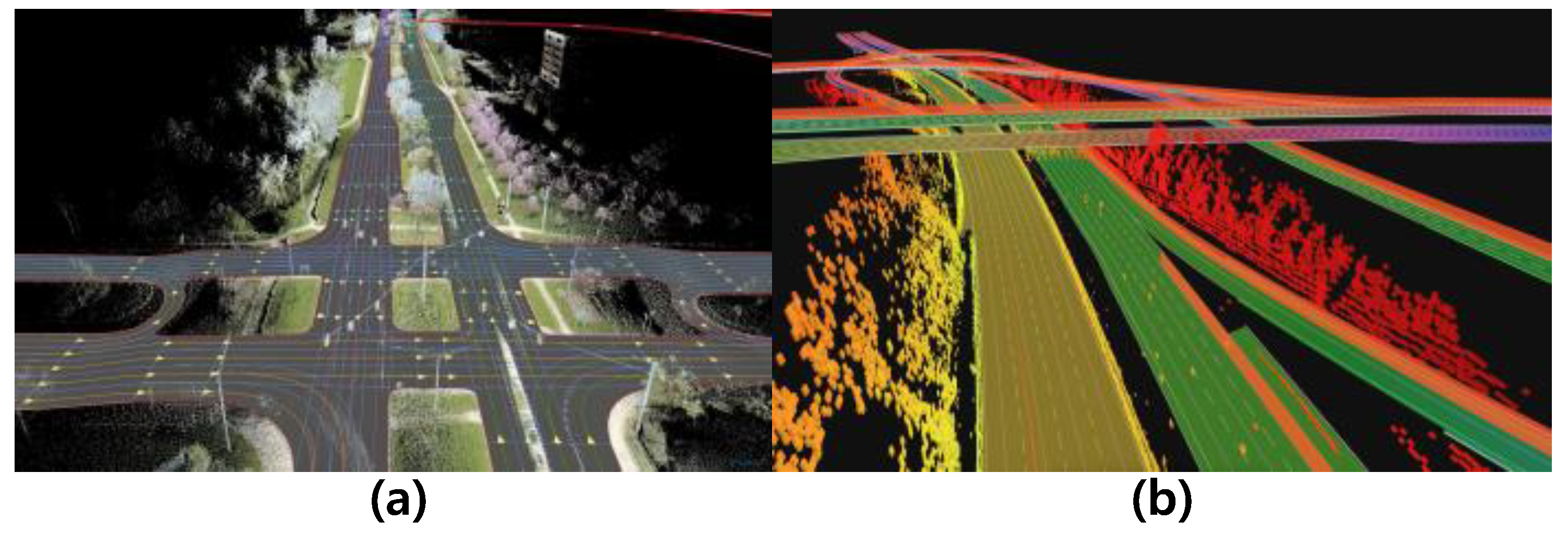
22], are preparing or starting to provide the HD map for the era of autonomous cars. HERE provides a HD map that contains various semantic features, such as road geometry, lane boundaries, barriers, traffic signs, and traffic lights, in 10-to-20 cm accuracy, as shown in
Figure 1a. TomTom also provides semantic features similar to HERE and provides depth information for static objects via Road DNA [
23], as shown in
Figure 1b.
A ground mapping is mainly used for the HD map building due to the high accuracy and reliability although aerial mapping is much cheaper and faster. The process of ground mapping consists of three steps: a data acquisition, a data processing, and a database management. The data acquisition is a process to collect the information about the physical environments by surveying with special mapping vehicles equipped with various mapping sensors such as a real-time kinematic (RTK)-GNSS, an inertial measurement unit (IMU), cameras, and lidars. After the data acquisition, the HD map features (static object, traffic control devices, and roadway geometry) are extracted through the data processing. The final step is the database management for providing a service of the map management and access. Due to these series of multiple processes, the mapping cost of HD map is much higher than the mapping of the topological map that is used for the in-car navigation module.
2.3. Problems of HD Map Changes
The most significant problem with the HD map is the change in the physical features. The change of physical feature can give the incorrect environment information to the autonomous driving system, and it can cause a negative impact on the safe autonomous driving. The localization based on the alignment of landmark perception and HD map also can be suffered from degradation of the accuracy and reliability due to a misalignment by the map changes. Therefore, the changes of HD map must be detected and managed by the autonomous driving system to prevent the performance degradation.
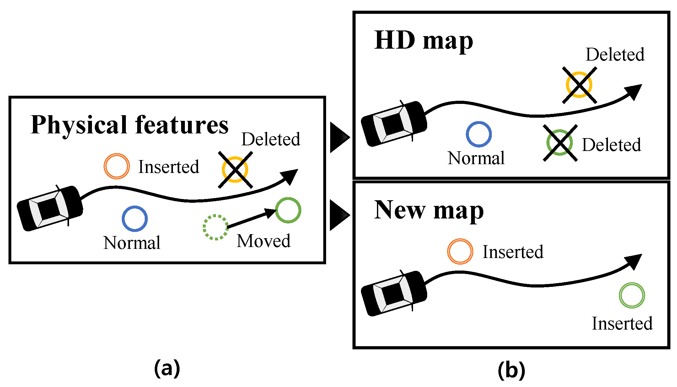
To detect and manage HD map change issues, we must clearly define what the HD map change is. There are three cases for the changes of the physical features on the road as shown in
Figure 2a: (1) a physical feature is moved; (2) a new physical feature is inserted; and (3) the physical feature is deleted. Since (1) the movement of physical features can be described as a series of (3) the deletion of physical feature and (2) the insertion of the new physical feature, we can define the changing physical feature as two classes that are a new physical feature and deleted physical feature. To reflect the physical feature changes to the HD map-based autonomous driving, we can classify the map features into three classes. The map features on the HD map can be classified into (1) normal map feature
and (2) deleted map feature
. To deal with the insertion of the new physical feature, a new map is required to manage the (3) new map feature
, as shown in
Figure 2b.
3. Simultaneous Localization and Map Change Update(SLAMCU) for HD Map
3.1. Management of the HD Map Changes by Individual Autonomous Vehicles
There are two ways to keep the up-to-date HD map that reflects physical feature changes. The first method is applying the ground mapping based on the special mapping vehicles to the map change detection and update. The special mapping vehicles survey all roads to collect the mapping data, the map feature changes are detected in the data processing step, and the changed map features are uploaded to map database. However, the ground mapping-based map change update is too expensive and not agile because it is based on the special mapping vehicles with limited frequency and range of operation.
The second way to recognize and update the HD map changes is to use the perception and localization of individual autonomous cars (or intelligent vehicles with the perception and localization capabilities) driving on the road. This method is more cost-effective than the first because there is no need to operate special mapping vehicles to monitor map changes. In addition, the HD map can keep up to date with the latest information because the map change update can be performed by multiple autonomous vehicles at the same time.
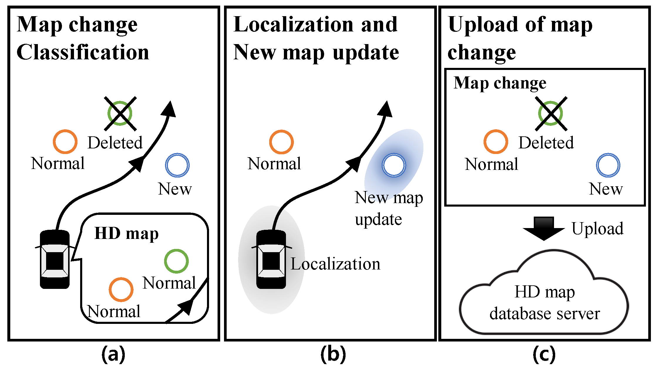
The process of the map change update based on the individual autonomous cars can be divided into three steps as shown in
Figure 3. The first step is a map change classification based on the physical features perception and the localization. The map features in the HD map is classified into the normal HD map feature
and the deleted HD map feature
. The new physical features that are not in the HD map are classified to the new map feature
. The second step is to utilize the classified features into the autonomous driving. The
is used for the autonomous driving and localization of autonomous vehicles. Conversely, the
has no effect on the autonomous driving and localization. For the new map feature
, the autonomous car should estimate the state (position) of the
, concurrently use for the autonomous driving and localization. The algorithm for the first and second step is Simultaneous Localization and Map Change Update (SLAMCU). The final step is reporting and uploading the map changes to the HD map database server (map provider). For the updating to the map server, we can apply a standard map update protocol such as SENSORIS [
24].
However, there are constraints of the individual vehicles based map change update due to the performance limitation of localization and perception on the vehicles. The perception limitation can cause the misclassification of the map feature changes, and the state estimation of new map features have poor accuracy compared to the mapping with special mapping vehicles. Nevertheless, the map change update based on the individual vehicles is worth because it can provide the probable location of map changes to the map provider, and it can supply the temporary information of the new map features that can be used before the mapping with the special mapping vehicles.
3.2. Analysis the SLAMCU Using Graph Structure
The simultaneous localization and map change update (SLAMCU) has two major functional requirements. The first requirement is to classify the HD map features into the normal and the deleted , and to only apply the normal feature for the localization and autonomous driving. The second functional requirement is to find the unregistered new physical feature, to register the found physical feature to new map feature , to estimate the state of the , and to apply the to the localization and autonomous driving. To design and implement the functional requirements of the SLAMCU based on the probabilistic framework, we analyze the SLAMCU problem using the graph of dynamic Bayesian networks (DBN).
A directed graph of a DBN based on the Markov process assumption can represent the various types of localization and mapping problems using the probabilistic framework. The DBN is composed of nodes for probabilistic random variables and directed edges for representing conditional dependencies between two nodes. The nodes of the localization and mapping problems consist of the , , , and . The indicates a sequence of the vehicle pose from discrete time steps 1 to t. The represents the vehicle motion input, and the represents the observation of the map features by perception sensors. The indicates the position of map features that can be observed by the perception of autonomous cars. The edges that represent probabilistic constraints between the nodes consists of a and for the localization and mapping problems. The represents a motion constraint between the two adjacent vehicle state and regarding the motion control input . The state transition model can predict the future vehicle state using the previous state and input . The describes the probability of measurement given the state with the map m. The measurement model can estimate the probability distribution of the measurement based on the current state and map features m.
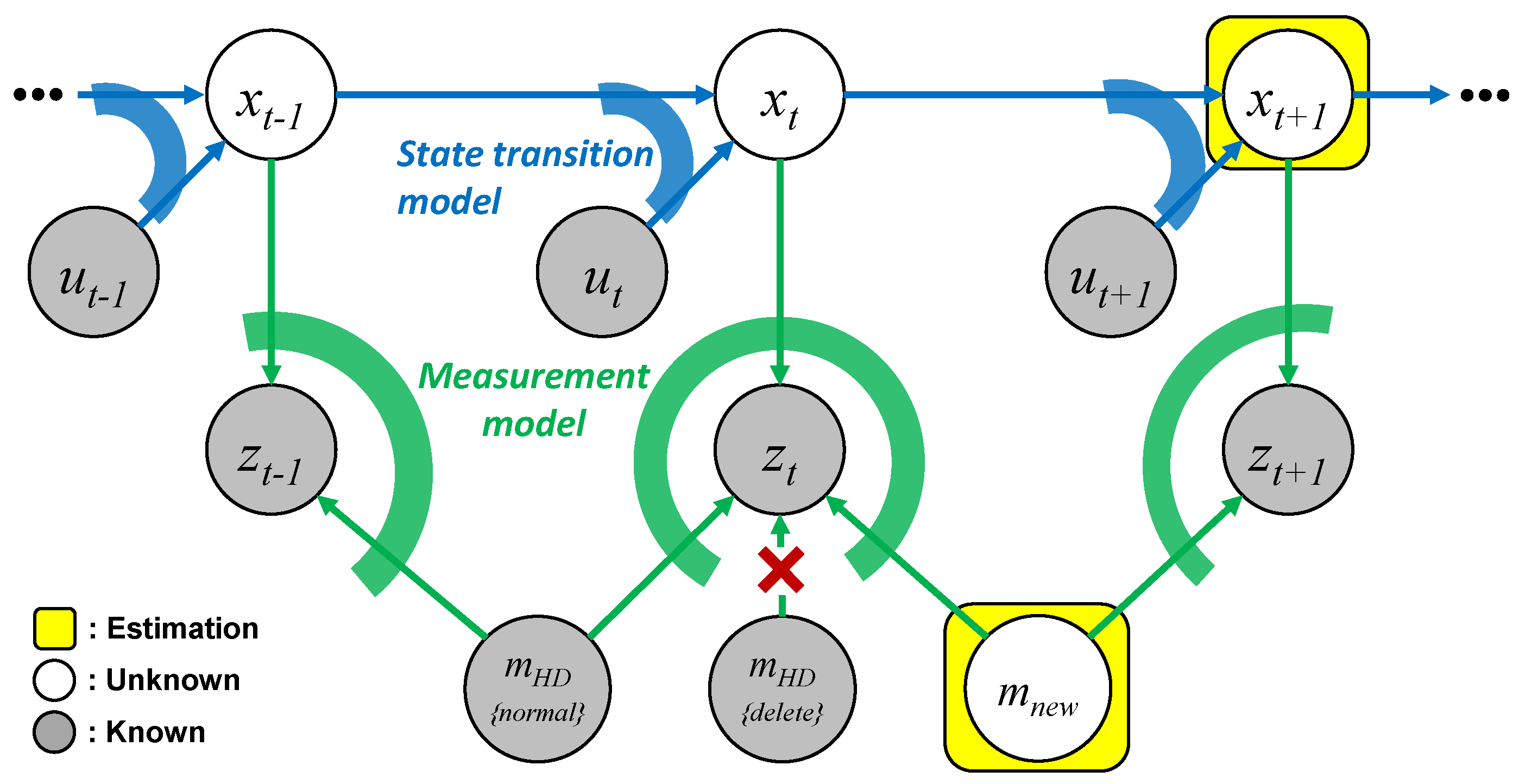
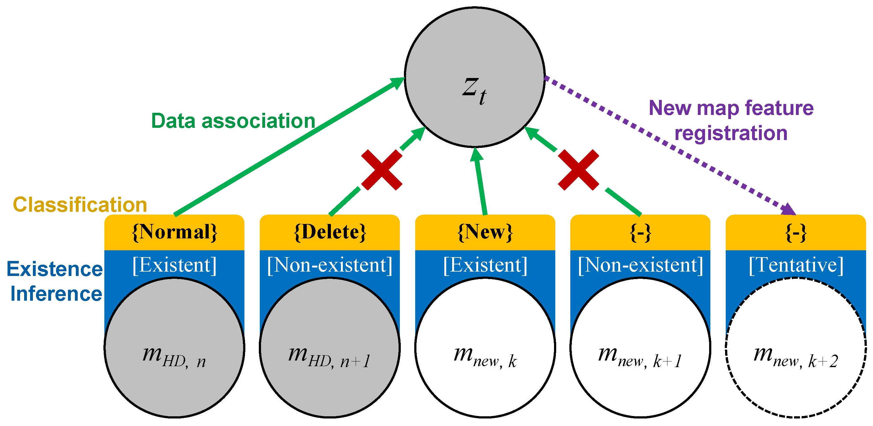
The SLAMCU problem can be interpreted by graph structure as shown in
Figure 4. The known nodes are input
, measurement
, and the map features
on HD map. The unknown nodes are state
and new map feature
. The SLAMCU wants to estimate the recent state
and the new map feature
based on the known nodes and the edge constraints. The first functional requirement of the SLAMCU can be represented through the graph structure as a localization problem with a data association. The localization estimates the state
using the input
, measurement
, and the HD map features
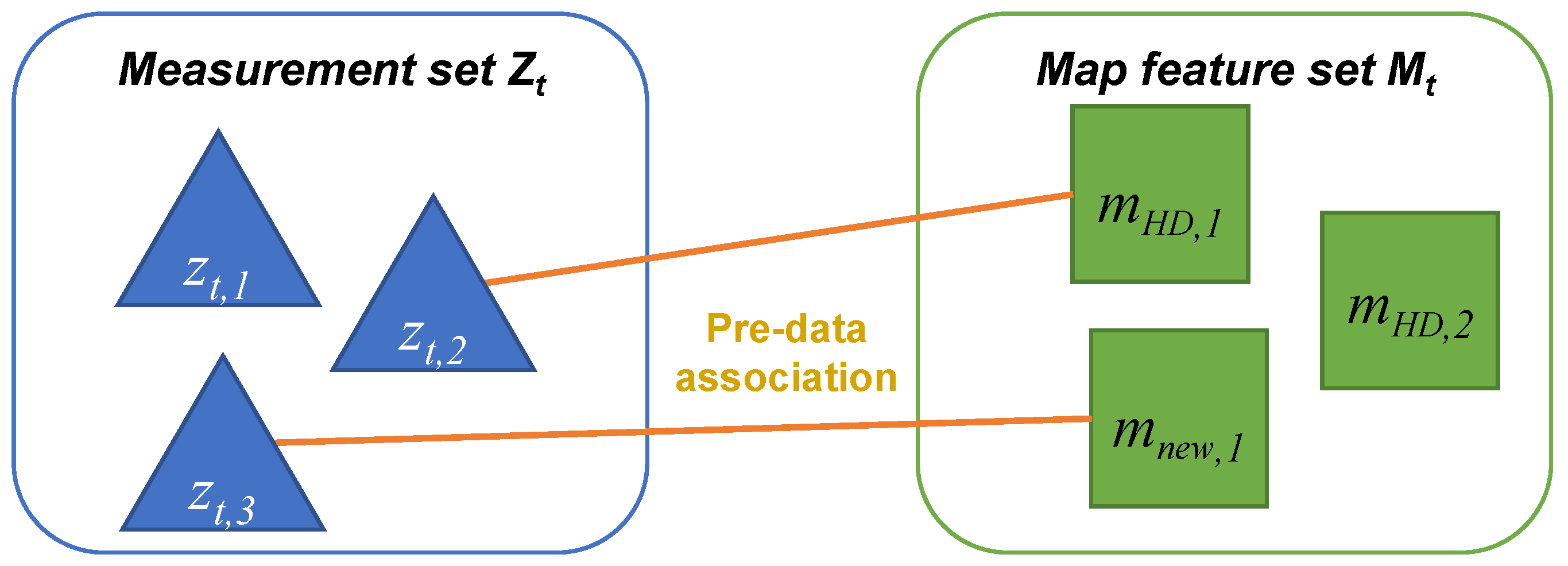
. The existence inference-based map management system generates links between the measurement
and the normal HD map features
by the edge of the measurement model, and disconnects the
to the deleted HD map features
. The second functional requirement can be interpreted as a SLAM (Simultaneous Localization and Mapping) problem that concurrently estimate the state
and the new map feature
. The existence inference-based map management generates a new link between the measurement
and the new map features
by the measurement model edge. In conclusion, the SLAMCU can be designed and implemented by the combination of localization and SLAM with the map management based on the existence inference of the physical features.
5. SLAMCU Based on Rao–Blackwellized Particle Filter
The SLAMCU is a problem to estimate the unknown vehicle pose state
and new map features
based on the known control input
, measurement
, and the HD map features
. Therefore, the SLAMCU can be represented in the posterior of conditional probability as described in (
8).
The Equation (
8) can be factorized into (
9).
If the
contains the
N number of features, the (
9) can be represented into (
10).
A Rao–Blackwellized particle filter (RBPF) can be applied to implement the posterior (
10). The RBPF is a combination of the standard particle filter and the Kalman filter. Because of the hybrid characteristics of the RBPF, it is available to take the both advantages of the particle filter and Kalman filter. Therefore, there were many studies to use the RBPF for localization and mapping [
25,
26,
27]. Among these previous studies, FastSLAM is the most successful SLAM implementation based on the RBPF [
28]. Therefore, the SLAMCU implementation follows the FastSLAM framework; however, the different things with the FastSLAM are (1) the SLAMCU take into account the HD map and (2) the map management system is needed to manage the HD map changes and new map features.
The SLAMCU based on the RBPF uses particle filter to estimate the posterior of vehicle pose state . For the new map feature , the SLAMCU uses Extended Kalman filter (EKF) to estimate the posterior of .
The particles
in SLAMCU are described as
where
is the index of particle,
and
are the mean and variance of the Gaussian model of the
n-th new map feature location. The total number of particles is
M, so the range of the index
k is from 1 to
M. The process of the SLAMCU based on the RBPF consists of four steps: a prediction, an update of a new map feature, an importance weighting, and a resampling.
5.1. Prediction
At the prediction step, the new sample state
of each particle
k is predicted by applying the state transition model to the previous state
with control input
, as described in (
12).
The state transition model can be implemented by vehicle motion models, such as kinematic and dynamic vehicle models, that have uncertainty characteristics for the control input and model prediction accuracy.
5.2. Updating the Estimate of New Map Features
The next step is to update the estimate of
n-th new map features
for each particle. The
n-th new map feature for each particle can be modeled by a Gaussian probability function, as described in (
13).
Before the update, a map management process is necessary (1) to detect the new physical features that are not registered on the HD map; (2) to infer the existence of the new map feature; and (3) to associate the perceptual measurement with the new map feature.
For the non-associated map features to the measurement
, the estimate of the new map feature is not updated as:
For the associate map feature to the measurement
, the posterior of the new map feature can be updated using
where
is the normalization factor. The
can be represented by Gaussian model of the previous step mean and covariance
. The posterior of new map feature
can be updated based on the linearlization technique of the EKF measurement update for the measurement model
, as described in
The is the index of the associated map feature with measurement , the R is the measurement covariance matrix, the h represents the function of the measurement model, the H is the Jacobian of the measurement model h, and the K is the Kalman gain for updating the new map feature.
5.3. Importance Weight
The weight
of each particle should be updated by evaluating the likelihood of perceptual measurement
. For the importance weight of the SLAMCU, there are two types of the measurement likelihoods that one is conditioned on the HD map feature
and the other is conditioned on the new map feature
. The weight for the likelihood conditioned on the HD map feature
can be calculated as
where
. The weight for likelihood conditioned on the new map feature
can be calculated as
where
. The weight
of each particle can be updated using the equation:
5.4. Resampling
Resampling is performed to randomly generate the new set of particles according to the importance weight of particles. The purpose of the particle resampling is to prevent the weight concentration of the few particles. The resampling is performed only if the following condition is satisfied:
is the effective number of samples that represents the degree of depletion. When all the particles have even weight values, the has the same value with a number of particles M. In contrast, when all the weights are concentrated to a single particle, the has its minimum value of one. The scale factor is selected according to the probabilistic characteristics of the particle filter.
6. Experiments
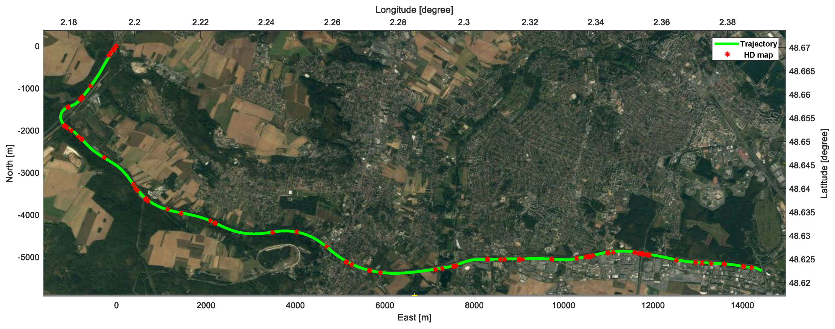
An experiment was conducted to evaluate the SLAMCU in the real driving situation of 20 km-long highway of France, as shown in
Figure 7. The SLAMCU algorithm is able to be applied to many types of features in the HD map, such as lane marking, guardrail, traffic light, and traffic sign. We selected the traffic sign as the validation feature of the SLAMCU because it is straightforward to qualitatively evaluate the proposed algorithm.
6.1. Experimental Environment
In order to evaluate the algorithm in the real in-vehicle environment, the traffic signs are measured by a commercial camera which is installed in mass-product vehicles. The camera performs the image processing at 15 FPS to measure the objects in the horizontal view of 40° and the detection range of 80 m. The measurements are transmitted by the CAN bus with 500 Kbps. A HD map produced by HERE offered the position information of the traffic sign features. The traffic signs in the map include lots of information such as position, size, shape, facing orientation, and type. Using the measurements and prior map information, the algorithm performs the RBPF including localization and map change update. The computer with a processor Intel(R) Core(TM) i5-4670 3.40 GHz and 16 GB of RAM takes 30.39 ms on average to process the algorithm.
6.2. Existence Inference Based on the DS Theory
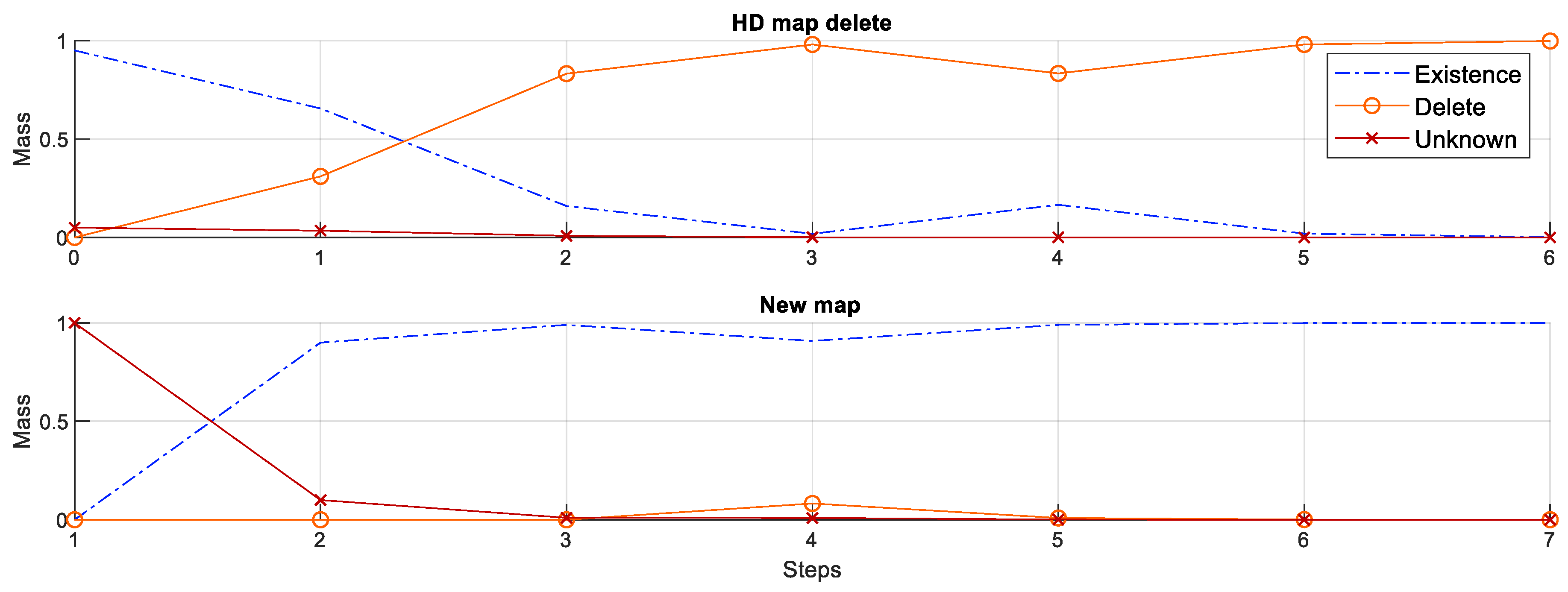
The changes of the map features are classified based on its existence. The existence could be evaluated by the mass functions of the power set based on the DS theory.
Figure 8 shows the mass functions of each existence state according to the sequence of the measurement input for cases of the deletion of HD map feature (upper figure) and the creation of new map feature (lower figure). To determine the deletion of HD map feature, the existence mass functions of the HD map feature was initialized with the (
3) and updated based on the Dempster combination rule (
5) with the non-measurement existence (
2). The existence confidence
of the traffic sign detection was 0.9 and the existence confidence of HD map feature
was 0.95. For the creation of new map feature, the existence mass functions of the new map feature were initialized from the position of the measurement with the (
4) and updated based on the combination rule (
5) with the measurement existence (
1). Although there were outliers for step 4 of the both process, it did not affect the final classification of the map changes.
6.3. Classification of the Map Changes
Table 1 shows the confusion matrix to evaluate the classification performance of the SLAMCU for the changes to the HD map. The entire accuracy was 96.12% for the classification of normal, deleted, and new map features. The accuracy of the normal classification was about 98%, and the one missing was due to the visibility occlusion of the traffic sign by a large truck. If the perception sensor is not able to detect the physical features due to the occlusion, there is no way to update the HD map. Therefore, the SLAMCU algorithm automatically does not take into account the occluded features for the update. The classification accuracy of the new map features was 92%, and the wrong classifications occurred because there are not enough measurement sequence of the traffic signs due to the fast vehicle speeds and slow detection of cameras. The map features classified into new and delete were possible to report to the map provider for the reflection of the map changes. For the new map features, SLAMCU estimated the position of the new traffic signs based on the RBPF approach.
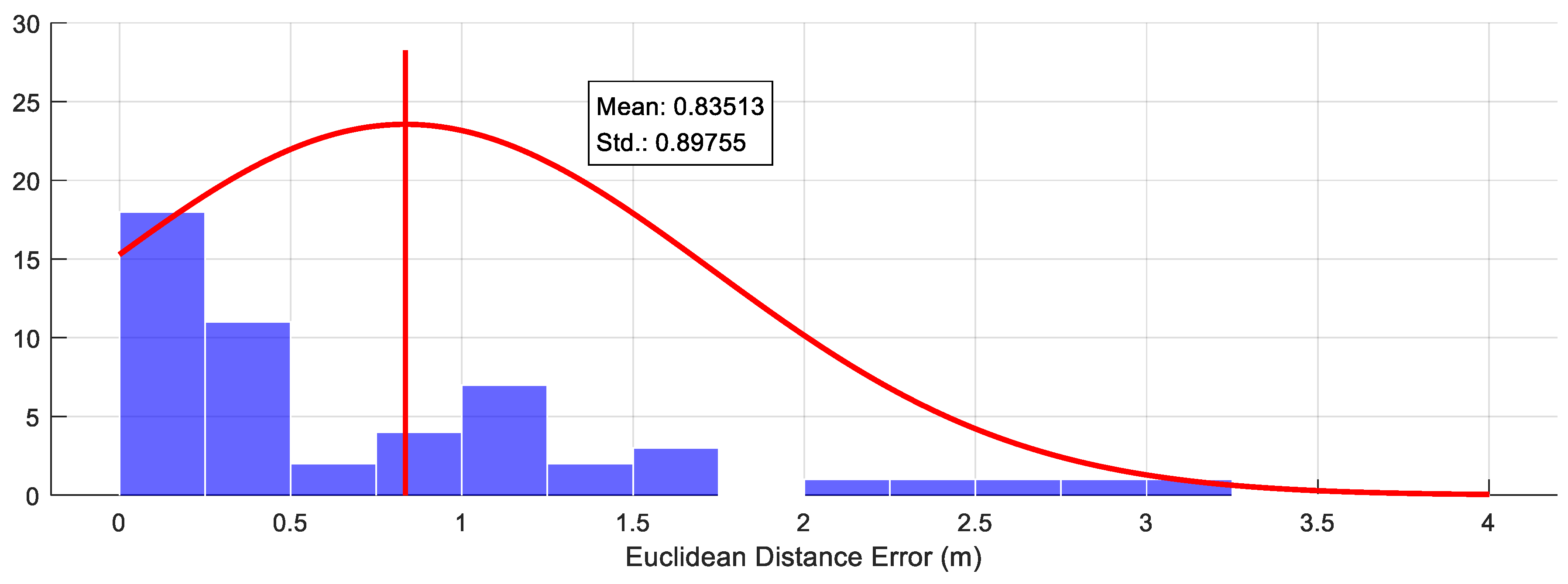
6.4. Estimation Accuracy of the New Map Features
The evaluation of position error for the traffic signs classified into the new map feature is shown in
Figure 8. The reference position of the new map features for the evaluation obtained by the GraphSLAM based post-processing with real-time Kinematics RTK-GPS. An average of the position error was about 0.8 m and the standard deviation was about 0.9 m, as shown in
Figure 9. The position error was caused by the uncertainty of the traffic sign detector using the camera vision. Although there was about one-meter error for the new feature estimation, it is enough to report the location of the map feature change to the map provider and use it as a temporary map feature until the precise ground mapping is performed.


