Energy-Efficient Online Resource Management and Allocation Optimization in Multi-User Multi-Task Mobile-Edge Computing Systems with Hybrid Energy Harvesting


 ,
,
Abstract
:1. Introduction
- We consider a multi-user multi-task MEC system with hybrid energy harvesting WDs to investigate the joint resource management and allocation problem. To solve the stochastic optimization problem, we turn the problem into two deterministic sub-problems, namely transmission optimization sub-problem and battery management sub-problems. The transmission optimization sub-problem can be designed to solve the transmission power and the transmission time of data, while the battery management sub-problem can be constructed to solve the needed wireless energy amount.
- Based on Lyapunov optimization theory and convex optimization theory, we use the proposed energy-efficient joint resource management and allocation algorithm (ECM-RMA) to solve the problem of minimizing energy consumption under delay guarantees. Without the prior knowledge, the algorithm allocates energy offloading data according to the energy harvest amount, remaining available time, amount of data to be processed and other factors at the beginning of each time slot.
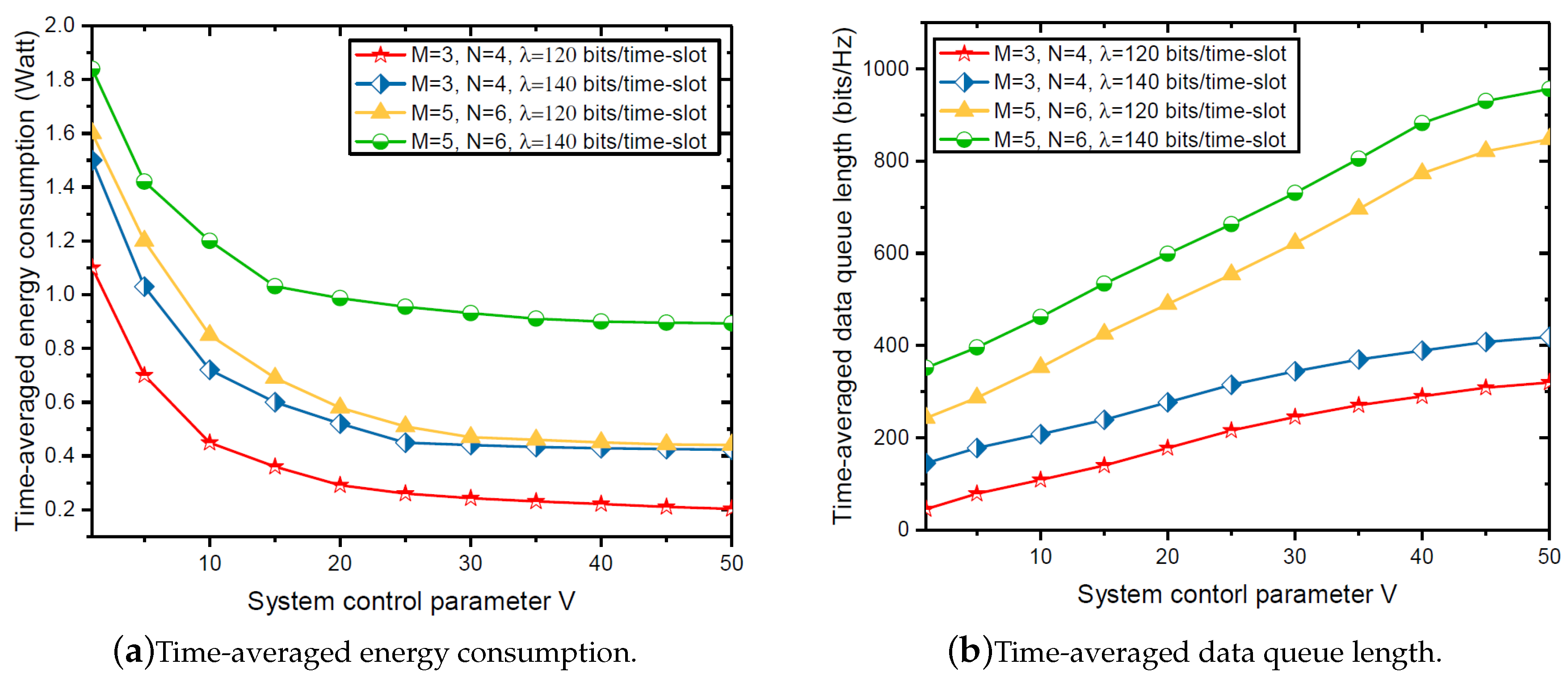
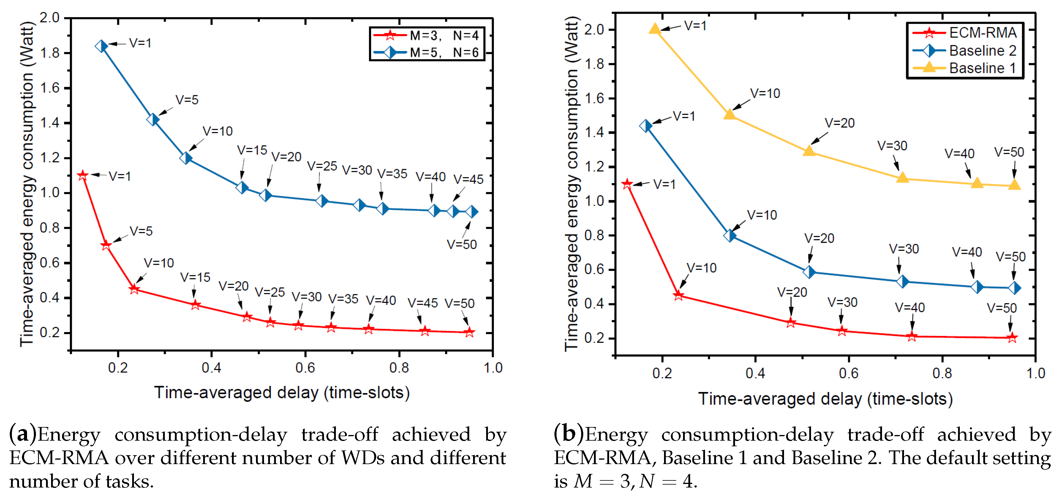
- The trade-off between energy consumption and delay is . V, as a non-negative weight, can achieve the balance between energy consumption and task data queues.
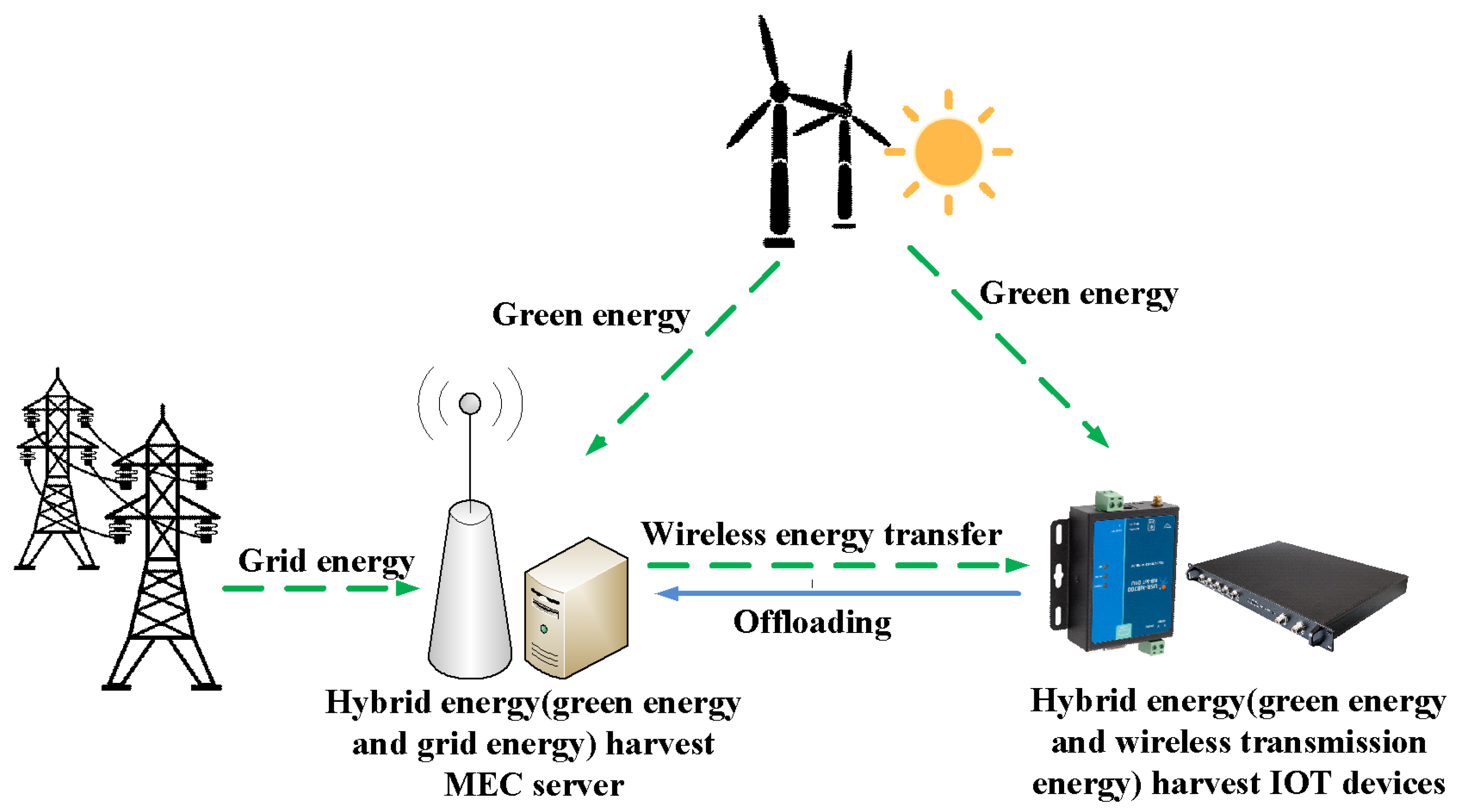
- In the field of MEC, we first proposed the devices with a hybrid energy harvesting method that integrates green energy and wireless energy.
2. Related Works
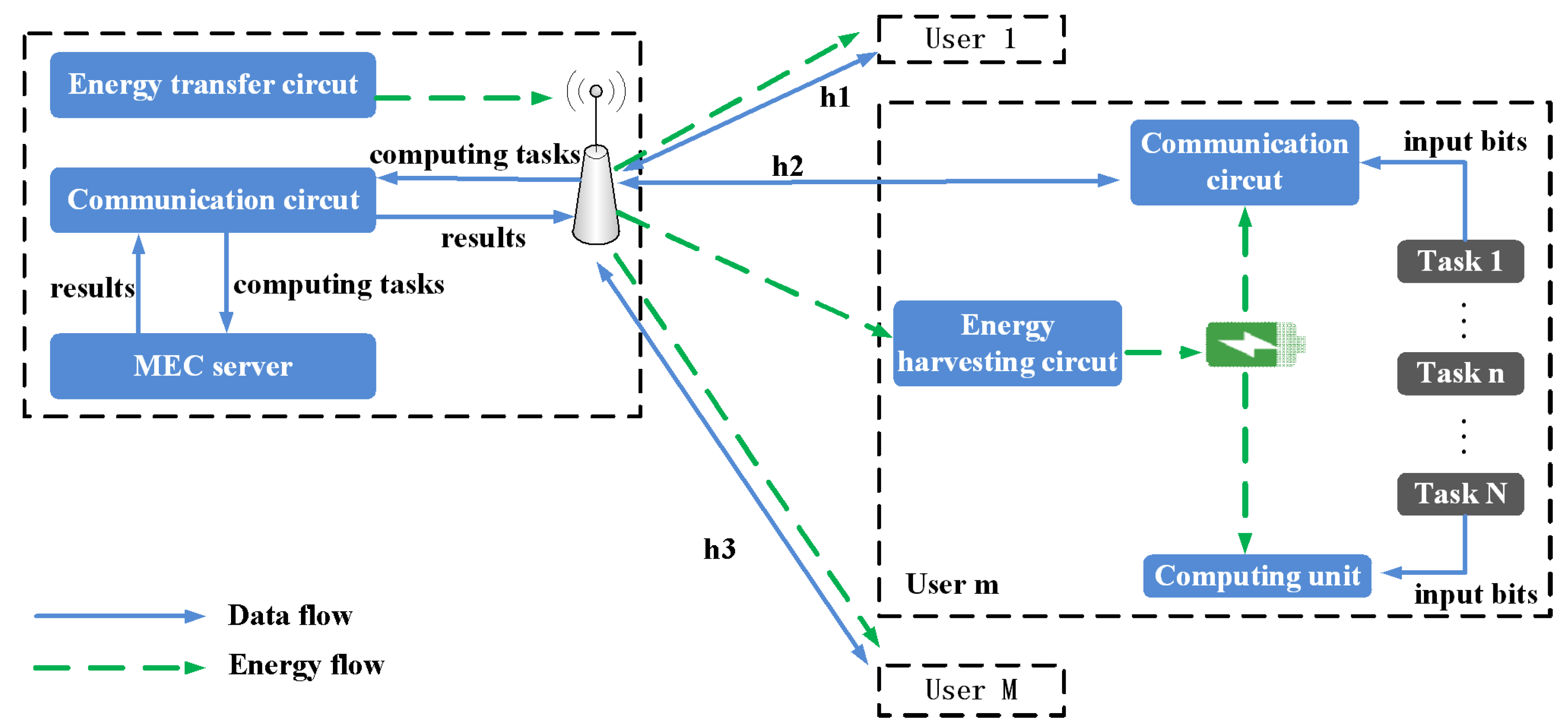
3. System Model
3.1. Communication Model
3.2. Task Computation Model
3.2.1. Local Computing
3.2.2. Mobile Edge Cloud Computing
3.3. Energy Consumption Model
3.4. Optimization Problem Formulation
4. Online Resource Management and Allocation Optimization in MEC
4.1. Lyapunov-Based Problem Decomposition
4.1.1. Transmission Optimization Problem
4.1.2. Battery Management Problem
4.2. Energy Consumption Minimization Resource Management and Allocation Algorithm (ECM-RMA)
| Algorithm 1 Proposed ECM-RMA algorithm | |
| Input: | |
| Output: | |
| 1: | Transmission Power and Transmission Time Allocation |
| 2: | fordo |
| 3: | for do |
| 4: | Solve the standard convex optimization problem in (35) to acquire the optimal power and time allocation policy; |
| 5: | end for |
| 6: | end for |
| 7: | Battery Management |
| 8: | fordo |
| 9: | if then |
| 10: | ; |
| 11: | ; |
| 12: | ; |
| 13: | ; |
| 14: | else |
| 15: | |
| 16: | end if |
| 17: | end for |
| 18: | Update the Queue Length |
| 19: | fordo |
| 20: | Compute based on Equation (11); |
| 21: | for do |
| 22: | Compute based on Equation (14); |
| 23: | end for |
| 24: | end for |
4.3. Performance Analysis
4.3.1. The Performance of the Proposed ECM-RMA Algorithm
4.3.2. The Trade-Off between Energy Consumption and Delay
5. Simulation Results
5.1. Simulation Settings in All Simulations, the Energy Transmitter at the AP with W
5.2. Performance Achieved by the ECM-RMA Algorithm
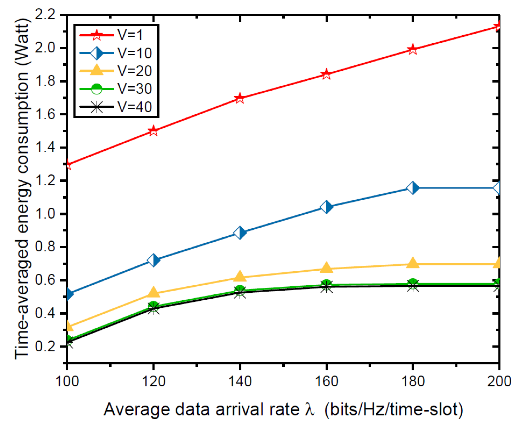
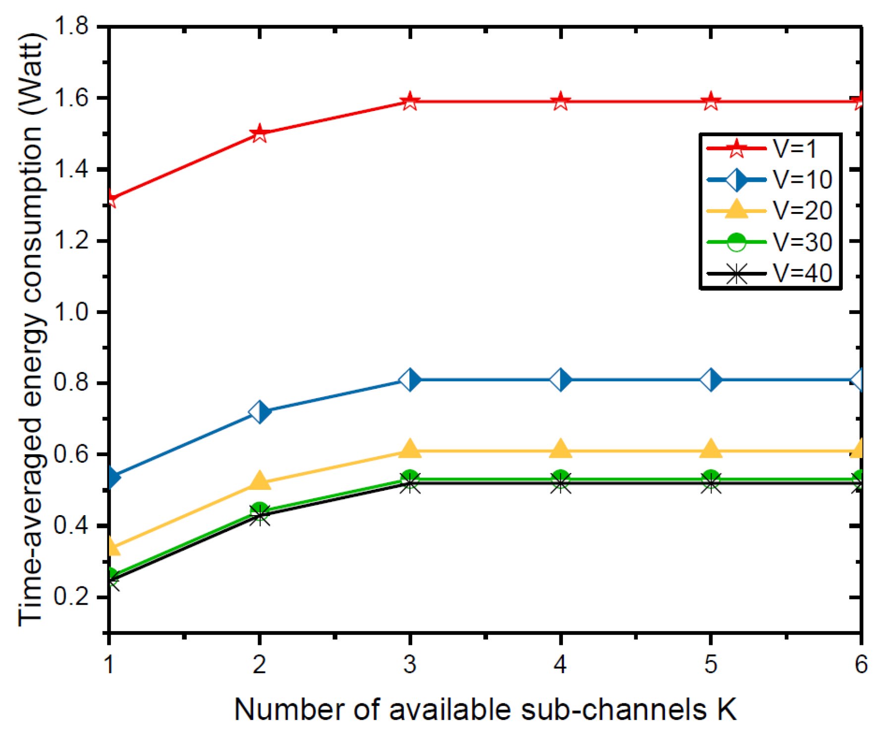
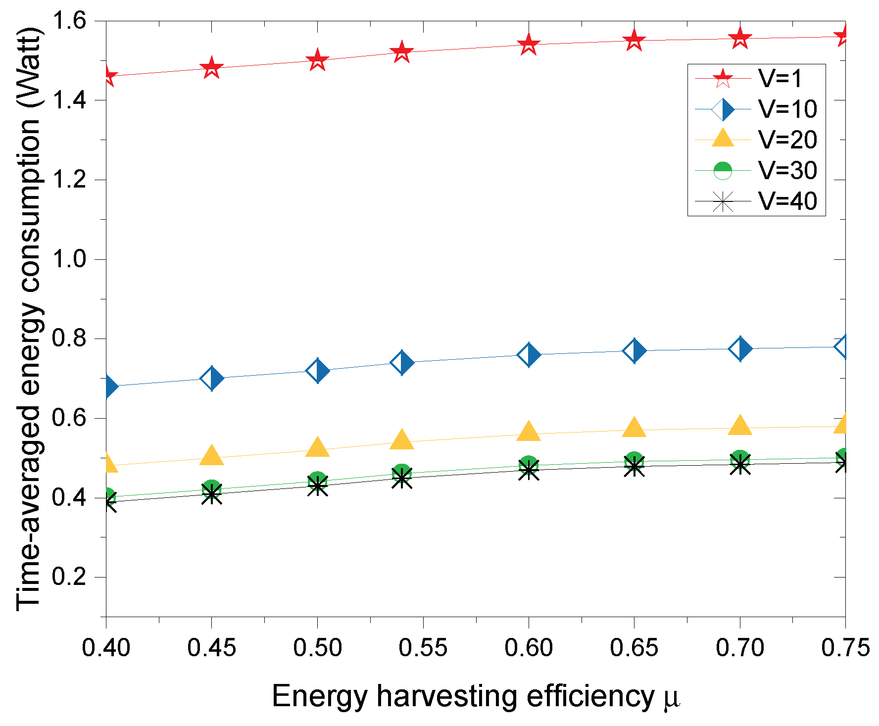
5.3. Impact of , K,
6. Conclusions
Author Contributions
Funding
Acknowledgments
Conflicts of Interest
Abbreviations
| MEC | mobile edge computing |
| WDs | wireless devices |
| IoT | Internet of Things |
| ECM-RMA | energy-efficient joint resource management and allocation |
| AP | access point |
| EH | energy harvesting |
| RF | radio frequency |
| WPT | wireless power transfer |
| MDP | Markov decision processes |
| eDors | energy-efficient dynamic offloading resource scheduling |
| i.i.d | independent and identically distributed |
| QoS | quality of service |
Appendix A. Proof of Lemma 1
Appendix B. Proof of Lemma 2
Appendix C. Proof of Theorem 1
Appendix D. Proof of Theorem 2
References
- Mao, S.; Leng, S.; Yang, K.; Zhao, Q.; Liu, M. Energy Efficiency and Delay Tradeoff in Multi-User Wireless Powered Mobile-Edge Computing Systems. In Proceedings of the GLOBECOM 2017–2017 IEEE Global Communications Conference, Singapore, 4–8 December 2017; pp. 1–6. [Google Scholar]
- Bi, S.; Zhang, Y.J.A. Computation Rate Maximization for Wireless Powered Mobile-Edge Computing with Binary Computation Offloading. IEEE Trans. Wirel. Commun. 2017, 17, 4177–4190. [Google Scholar] [CrossRef]
- Wu, J.; Chen, Z.; Zhao, M. Information cache management and data transmission algorithm in opportunistic social networks. Wirel. Netw. 2018, 1–12. [Google Scholar] [CrossRef]
- Park, D.; Kim, S.; An, Y.; Jung, J.Y. LiReD: A Light-Weight Real-Time Fault Detection System for Edge Computing Using LSTM Recurrent Neural Networks. Sensors 2018, 18, 2110. [Google Scholar] [CrossRef] [PubMed]
- Premsankar, G.; Francesco, M.D.; Taleb, T. Edge Computing for the Internet of Things: A Case Study. IEEE Internet Things J. 2018, 5, 1275–1284. [Google Scholar] [CrossRef]
- Wang, F.; Xu, J.; Wang, X.; Cui, S. Joint Offloading and Computing Optimization in Wireless Powered Mobile-Edge Computing Systems. IEEE Trans. Wirel. Commun. 2017, 17, 1784–1797. [Google Scholar] [CrossRef]
- Wu, J.; Chen, Z.; Zhao, M. Weight distribution and community reconstitution based on communities communications in social opportunistic networks. Peer-to-Peer Netw. Appl. 2018, 1–9. [Google Scholar] [CrossRef]
- Mahapatra, C.; Moharana, A.; Leung, V. Energy Management in Smart Cities Based on Internet of Things: Peak Demand Reduction and Energy Savings. Sensors 2017, 17, 2812. [Google Scholar] [CrossRef] [PubMed]
- Chen, Z.; Guo, L.; Zhang, D.; Chen, X. Energy and channel transmission management algorithm for resource harvesting body area networks. Int. J. Distrib. Sens. Netw. 2018, 14, 155014771875923. [Google Scholar] [CrossRef]
- Jia, W.U.; Chen, Z.; Zhao, M. Effective information transmission based on socialization nodes in opportunistic networks. Comput. Netw. 2017, 129, 297–305. [Google Scholar]
- Nan, Y.; Li, W.; Bao, W.; Delicato, F.C.; Pires, P.F.; Dou, Y.; Zomaya, A.Y. Adaptive Energy-aware Computation Offloading for Cloud of Things Systems. IEEE Access 2017, 5, 23947–23957. [Google Scholar] [CrossRef]
- Ko, S.W.; Kim, S.L. Impact of Node Speed on Energy-Constrained Opportunistic Internet-of-Things with Wireless Power Transfer. Sensors 2018, 18, 2398. [Google Scholar] [CrossRef] [PubMed]
- Yang, J.; Yang, Q.; Kwak, K.S.; Rao, R.R. Power–CDelay Tradeoff in Wireless Powered Communication Networks. IEEE Trans. Veh. Technol. 2017, 66, 3280–3292. [Google Scholar] [CrossRef]
- Wang, Y.; Sheng, M.; Wang, X.; Wang, L.; Li, J. Mobile-Edge Computing: Partial Computation Offloading Using Dynamic Voltage Scaling. IEEE Trans. Commun. 2016, 64, 4268–4282. [Google Scholar] [CrossRef]
- Kao, Y.H.; Krishnamachari, B.; Ra, M.R.; Bai, F. Hermes: Latency Optimal Task Assignment for Resource-constrained Mobile Computing. IEEE Trans. Mob. Comput. 2017, 16, 3056–3069. [Google Scholar] [CrossRef]
- Zhang, W.; Wen, Y.; Wu, D.O. Collaborative Task Execution in Mobile Cloud Computing Under a Stochastic Wireless Channel. IEEE Trans. Wirel. Commun. 2015, 14, 81–93. [Google Scholar] [CrossRef]
- Khalili, S.; Simeone, O. Inter-layer per-mobile optimization of cloud mobile computing: A message-passing approach. Trans. Emerg. Telecommun. Technol. 2016, 27, 814–827. [Google Scholar] [CrossRef]
- Lorenzo, P.D.; Barbarossa, S.; Sardellitti, S. Joint Optimization of Radio Resources and Code Partitioning in Mobile Edge Computing. arXiv, 2013; arXiv:1307.3835. [Google Scholar]
- Mahmoodi, S.E.; Subbalakshmi, K.P.; Sagar, V. Cloud offloading for multi-radio enabled mobile devices. In Proceedings of the 2015 IEEE International Conference on Communications (ICC), London, UK, 8–12 June 2015; pp. 5473–5478. [Google Scholar]
- You, C.; Huang, K.; Chae, H.; Kim, B.H. Energy-Efficient Resource Allocation for Mobile-Edge Computation Offloading. IEEE Trans. Wirel. Commun. 2017, 16, 1397–1411. [Google Scholar] [CrossRef]
- Barbarossa, S.; Sardellitti, S.; Lorenzo, P.D. Joint allocation of computation and communication resources in multiuser mobile cloud computing. In Proceedings of the 2013 IEEE 14th Workshop on Signal Processing Advances in Wireless Communications (SPAWC), Darmstadt, Germany, 16–19 June 2013; Volume 395, pp. 26–30. [Google Scholar]
- Chen, X.; Jiao, L.; Li, W.; Fu, X. Efficient Multi-User Computation Offloading for Mobile-Edge Cloud Computing. IEEE/ACM Trans. Netw. 2016, 24, 2795–2808. [Google Scholar] [CrossRef]
- Lyu, X.; Tian, H.; Sengul, C.; Zhang, P. Multiuser Joint Task Offloading and Resource Optimization in Proximate Clouds. IEEE Trans. Veh. Technol. 2017, 66, 3435–3447. [Google Scholar] [CrossRef]
- Mao, Y.; Zhang, J.; Song, S.H.; Letaief, K.B. Power-Delay Tradeoff in Multi-User Mobile-Edge Computing Systems. In Proceedings of the 2016 IEEE Global Communications Conference (GLOBECOM), Washington, DC, USA, 4–8 December 2016. [Google Scholar]
- Guo, S.; Xiao, B.; Yang, Y.; Yang, Y. Energy-efficient dynamic offloading and resource scheduling in mobile cloud computing. In Proceedings of the IEEE INFOCOM 2016—The IEEE International Conference on Computer Communications, San Francisco, CA, USA, 10–14 April 2016; pp. 1–9. [Google Scholar]
- Yu, Y.; Zhang, J.; Letaief, K.B. Joint Subcarrier and CPU Time Allocation for Mobile Edge Computing. In Proceedings of the 2016 IEEE Global Communications Conference (GLOBECOM), Washington, DC, USA, 4–8 December 2016; pp. 1–6. [Google Scholar]
- Zhao, T.; Zhou, S.; Guo, X.; Zhao, Y. A Cooperative Scheduling Scheme of Local Cloud and Internet Cloud for Delay-Aware Mobile Cloud Computing. In Proceedings of the 2015 IEEE Globecom Workshops (GC Wkshps), San Diego, CA, USA, 6–10 December 2015; pp. 1–6. [Google Scholar]
- Chen, M.H.; Dong, M.; Liang, B. Joint offloading decision and resource allocation for mobile cloud with computing access point. In Proceedings of the 2016 IEEE International Conference on Acoustics, Speech and Signal Processing (ICASSP), Shanghai, China, 20–25 March 2016; pp. 3516–3520. [Google Scholar]
- Xu, J.; Ren, S. Online Learning for Offloading and Autoscaling in Renewable-Powered Mobile Edge Computing. In Proceedings of the 2016 IEEE Global Communications Conference (GLOBECOM), Washington, DC, USA, 4–8 December 2016; pp. 1–6. [Google Scholar]
- Mao, Y.; Zhang, J.; Letaief, K.B. Dynamic Computation Offloading for Mobile-Edge Computing With Energy Harvesting Devices. IEEE J. Sel. Areas Commun. 2016, 34, 3590–3605. [Google Scholar] [CrossRef]
- Hao, Y.; Chen, M.; Hu, L.; Hossain, M.S.; Ghoniem, A. Energy Efficient Task Caching and Offloading for Mobile Edge Computing. IEEE Access 2018, 6, 11365–11373. [Google Scholar] [CrossRef]
- Li, Y.; Sheng, M.; Shi, Y.; Ma, X. Energy Efficiency and Delay Tradeoff for Time-Varying and Interference-Free Wireless Networks. IEEE Trans. Wirel. Commun. 2014, 13, 5921–5931. [Google Scholar] [CrossRef]
- Neely, M. Stochastic Network Optimization with Application to Communication and Queueing Systems. Synth. Lect. Commun. Netw. 2010, 3, 1–211. [Google Scholar] [CrossRef]
- Li, Y.; Sheng, M.; Wang, C.X.; Wang, X.; Shi, Y.; Li, J. Throughput–Delay Tradeoff in Interference-Free Wireless Networks With Guaranteed Energy Efficiency. IEEE Trans. Wirel. Commun. 2015, 14, 1608–1621. [Google Scholar] [CrossRef]
- Zhang, K.; Mao, Y.; Leng, S.; Zhao, Q.; Li, L.; Peng, X.; Pan, L.; Maharjan, S.; Zhang, Y. Energy-Efficient Offloading for Mobile Edge Computing in 5G Heterogeneous Networks. IEEE Access 2017, 4, 5896–5907. [Google Scholar] [CrossRef]


| Notation | Defination |
|---|---|
| The set of WDs | |
| The set of tasks | |
| The set of time slots | |
| The uplink transmission power between WD m and the AP at time slot t | |
| The uplink channel gains between WD m and the AP at time slot t | |
| The white noise power level of uplink channel | |
| The uplink channel bandwidth that the AP allocates for the WD m at time slot t | |
| The uplink transmission rate between WD m and the AP | |
| The duration of task n partially offloaded from WD m to the AP within time slot t | |
| The time allocated schedule of all tasks in WD m during slot t | |
| The amount of computation task arrived at user m at the end of the time slot t | |
| The CPU-cycle frequency assigned to task n on WD m at time slot t | |
| The CPU-cycles required to calculate one bit of data in WD m at time slot t | |
| The local computed data amount of task n of WD m at time slot t | |
| The energy consumption for local computation for task n of WD m during a time slot t | |
| The offloaded data amount of task n of WD m at time slot t | |
| The energy consumption of WD m offloading the data of task n at time slot t | |
| The total computed data of task n of WD m at time slot t | |
| The backlog of the data queue for task n of WD m at time slot t | |
| The energy obtained from the environment of WD m at time slot t | |
| The energy obtained from the AP of WD m at time slot t | |
| The total harvested energy of WD m at time slot t | |
| The energy supply from the environment at time slot t | |
| The total energy consumed by WD m for task n within time slot t | |
| The dynamic change of WD’s energy queue | |
| M | The number of WDs |
| N | The number of tasks in a WD |
| T | The slot length |
| S | The number of slots |
| K | The number of available sub-channel |
| The maximum uplink transmission power | |
| The minimum uplink transmission power | |
| The maximum arrive data | |
| The maximum green energy supply |
| Abbreviation | Defination |
|---|---|
| WD | Wireless device |
| WDs | Wireless devices |
| AP | Access point |
© 2018 by the authors. Licensee MDPI, Basel, Switzerland. This article is an open access article distributed under the terms and conditions of the Creative Commons Attribution (CC BY) license (http://creativecommons.org/licenses/by/4.0/).
Share and Cite
Zhang, H.; Chen, Z.; Wu, J.; Deng, Y.; Xiao, Y.; Liu, K.; Li, M. Energy-Efficient Online Resource Management and Allocation Optimization in Multi-User Multi-Task Mobile-Edge Computing Systems with Hybrid Energy Harvesting. Sensors 2018, 18, 3140. https://doi.org/10.3390/s18093140
Zhang H, Chen Z, Wu J, Deng Y, Xiao Y, Liu K, Li M. Energy-Efficient Online Resource Management and Allocation Optimization in Multi-User Multi-Task Mobile-Edge Computing Systems with Hybrid Energy Harvesting. Sensors. 2018; 18(9):3140. https://doi.org/10.3390/s18093140
Chicago/Turabian StyleZhang, Heng, Zhigang Chen, Jia Wu, Yiqing Deng, Yutong Xiao, Kanghuai Liu, and Mingxuan Li. 2018. "Energy-Efficient Online Resource Management and Allocation Optimization in Multi-User Multi-Task Mobile-Edge Computing Systems with Hybrid Energy Harvesting" Sensors 18, no. 9: 3140. https://doi.org/10.3390/s18093140
APA StyleZhang, H., Chen, Z., Wu, J., Deng, Y., Xiao, Y., Liu, K., & Li, M. (2018). Energy-Efficient Online Resource Management and Allocation Optimization in Multi-User Multi-Task Mobile-Edge Computing Systems with Hybrid Energy Harvesting. Sensors, 18(9), 3140. https://doi.org/10.3390/s18093140