A Flexible Wireless Sensor Network Based on Ultra-Wide Band Technology for Ground Instability Monitoring

 ,
, 
 ,
,  , , ,
, , , 
 ,
,  and
and 
Abstract
1. Introduction
1.1. Background and Motivation
1.2. Objectives and Project Framework
2. Materials and Methods
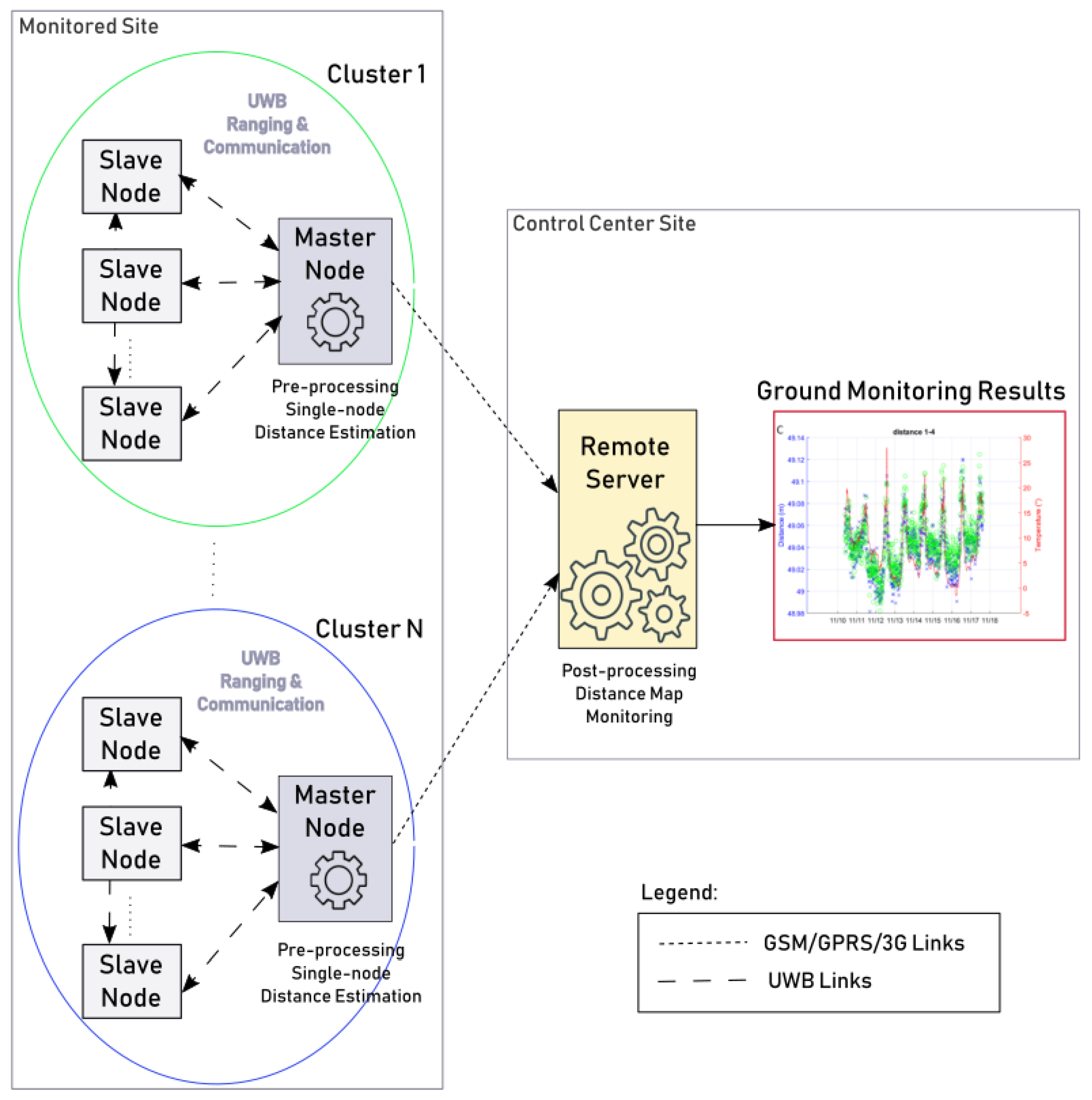
2.1. Wi-GIM System Architecture
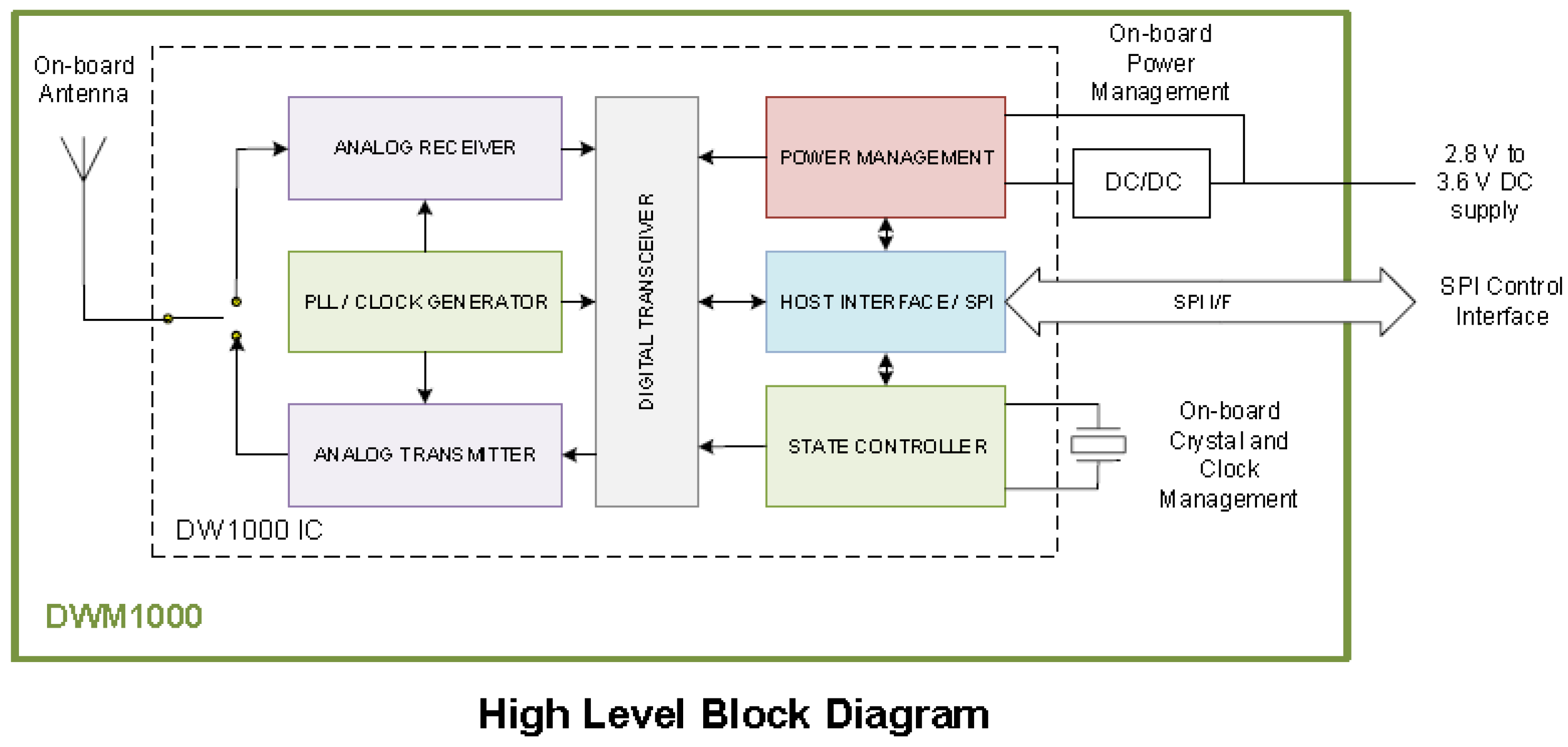
2.2. UWB Technology for Distance Estimation
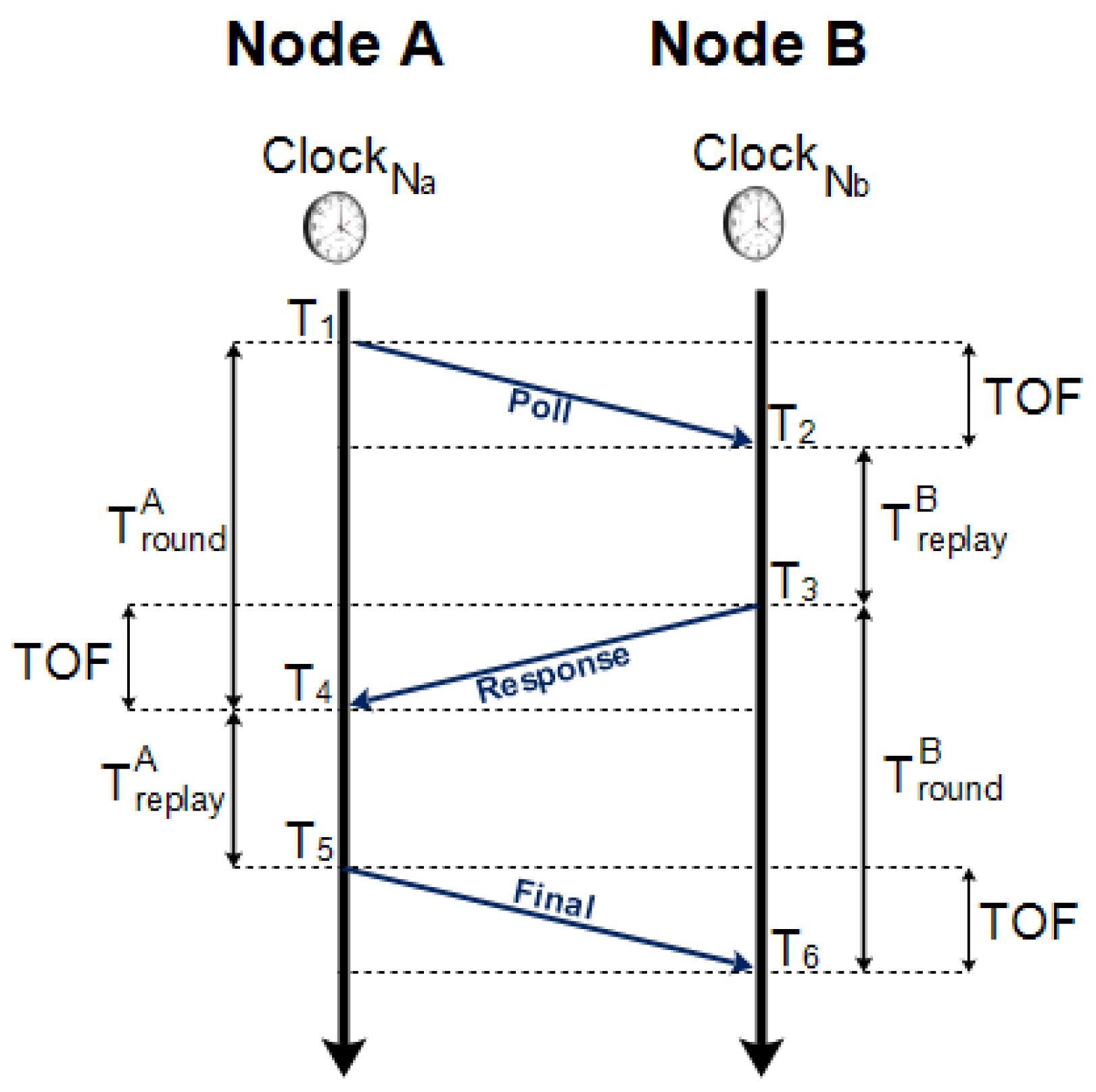
2.2.1. UWB Two-Way Ranging Technique
2.3. Wi-GIM Installation Procedure
2.4. Processing and Communication Protocols
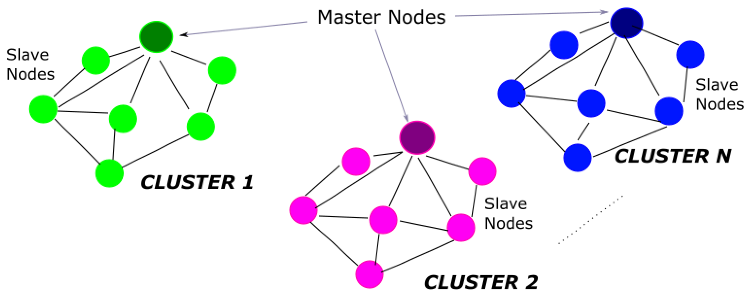
2.4.1. Network Initialization: Clustering Algorithm
2.4.2. On Site Master Node: Coordination and Pre-Processing
2.4.3. Remote Post-Processing
- outliers identification and removal (outlier filtering);
- temperature-dependent error correction;
- averaging over several measures (statistic filtering);
- constant offset correction.
3. Laboratory and Field Tests: Wi-GIM System Validation
- Laboratory tests. These tests aim to prove the nominal performance of the prototype.
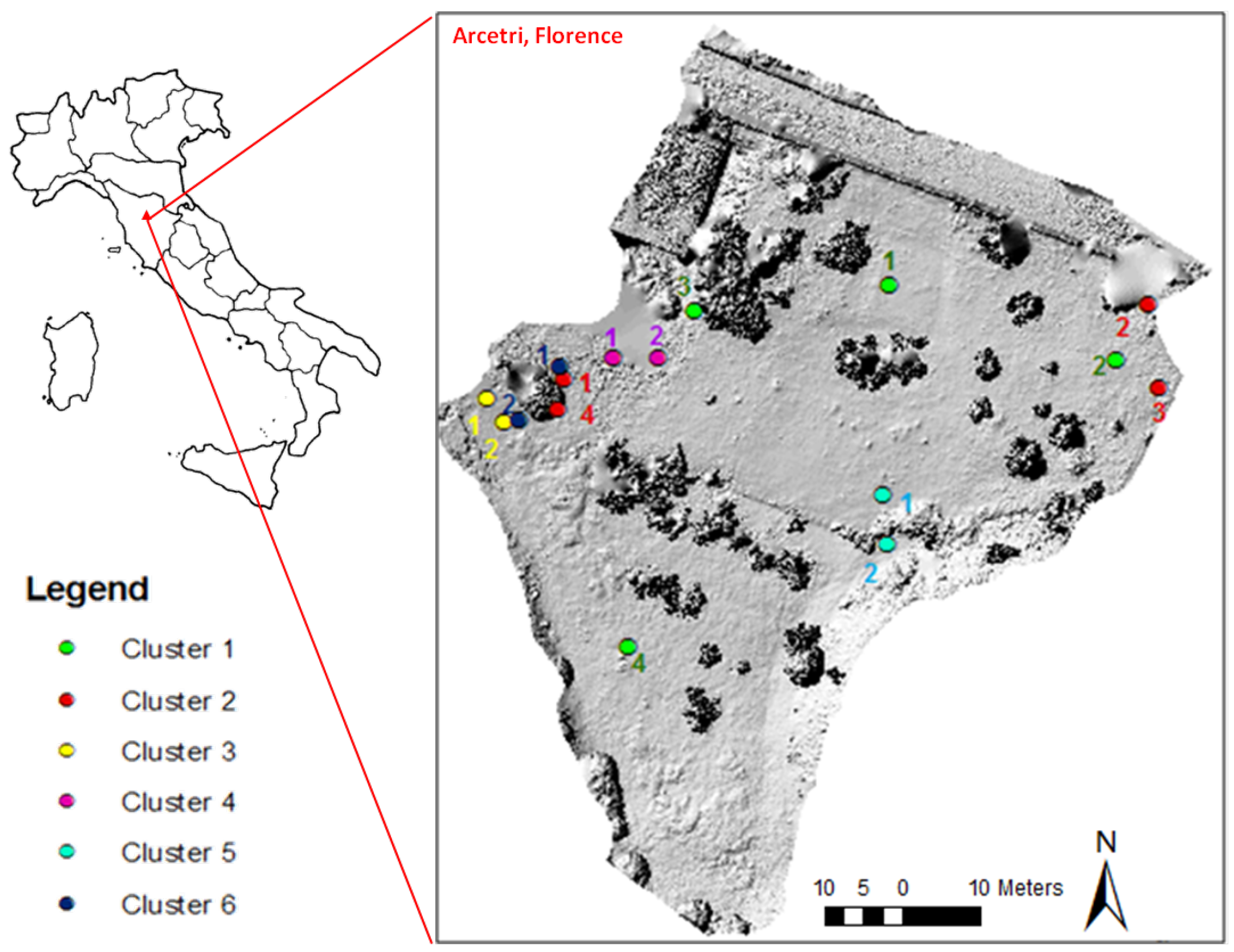
- Early calibration tests and sensitivity analyses. These tests aim at highlighting the system dependence to environmental and physical parameters (snow, rain, obstacles) and lead to the introduction of some technical improvements of the prototype (e.g., firmware redesign for battery management optimization—sleep mode, single hopping mode. They have been carried out in Arcetri, Florence (Central Italy) and result in a higher performance system level.
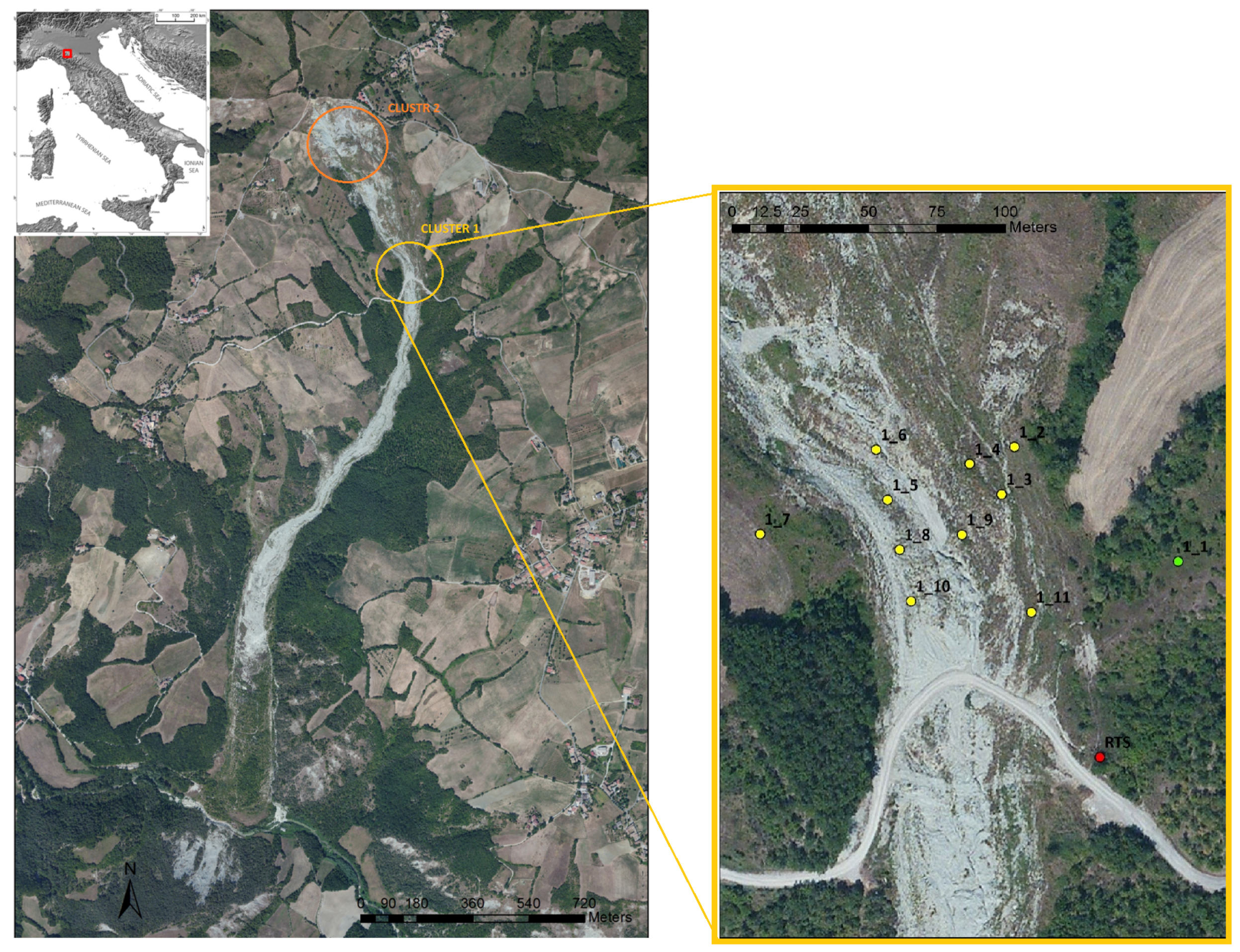
- Landslide application tests. A target site having different geomorphological characteristics has been considered: it is Roncovetro in Italy. It is characterized by a medium-fast moving landslide.
3.1. System Sensitivity Analyses (Arcetri)
3.2. Roncovetro Landslide Monitoring
4. Results
4.1. UWB Distance Estimation and Accuracy
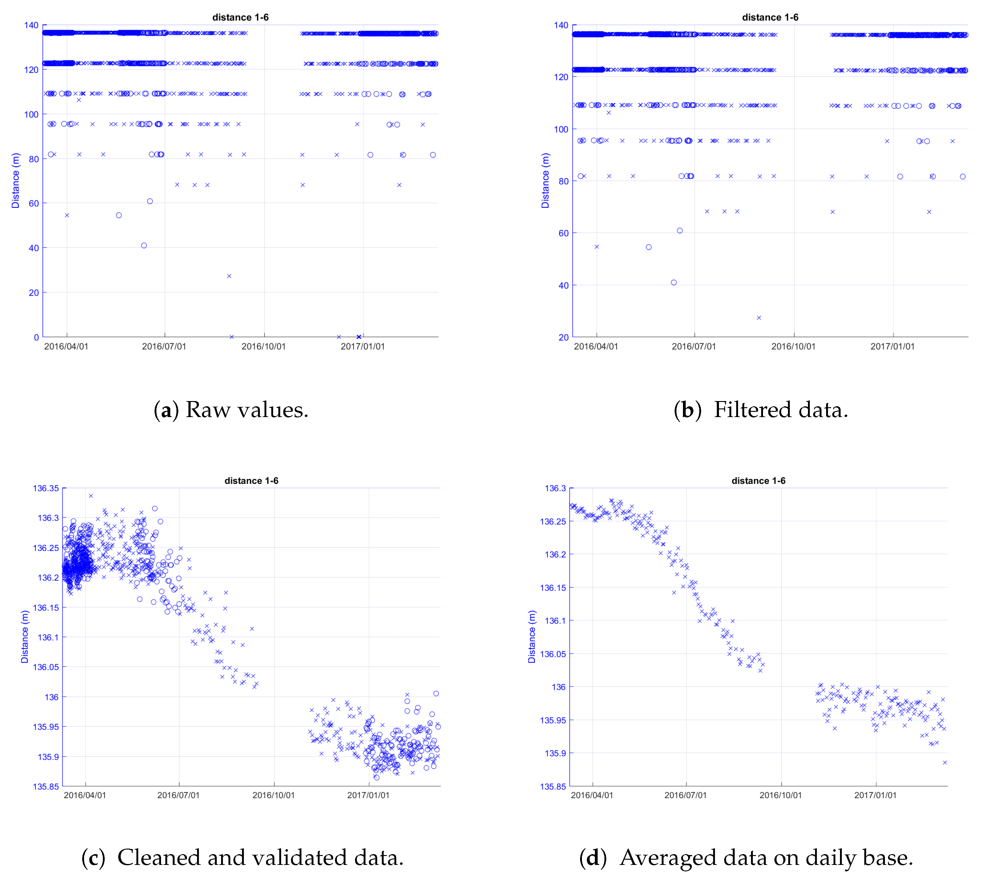
4.1.1. UWB Ranging Measurement Filtering
4.1.2. UWB and RTS Ranging Measurement Comparison
4.1.3. UWB and CWR Precision Performance
4.2. Analysis of the Influence Factors Effects on Distance Estimation
4.2.1. LOS/NLOS Condition Effect
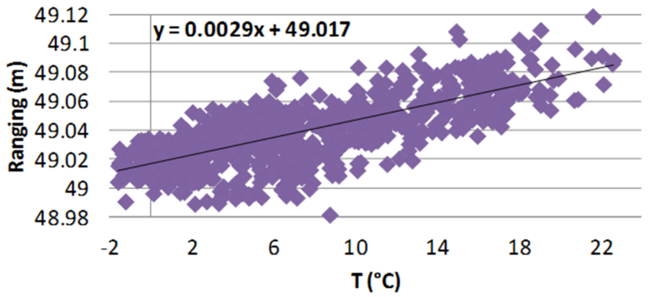
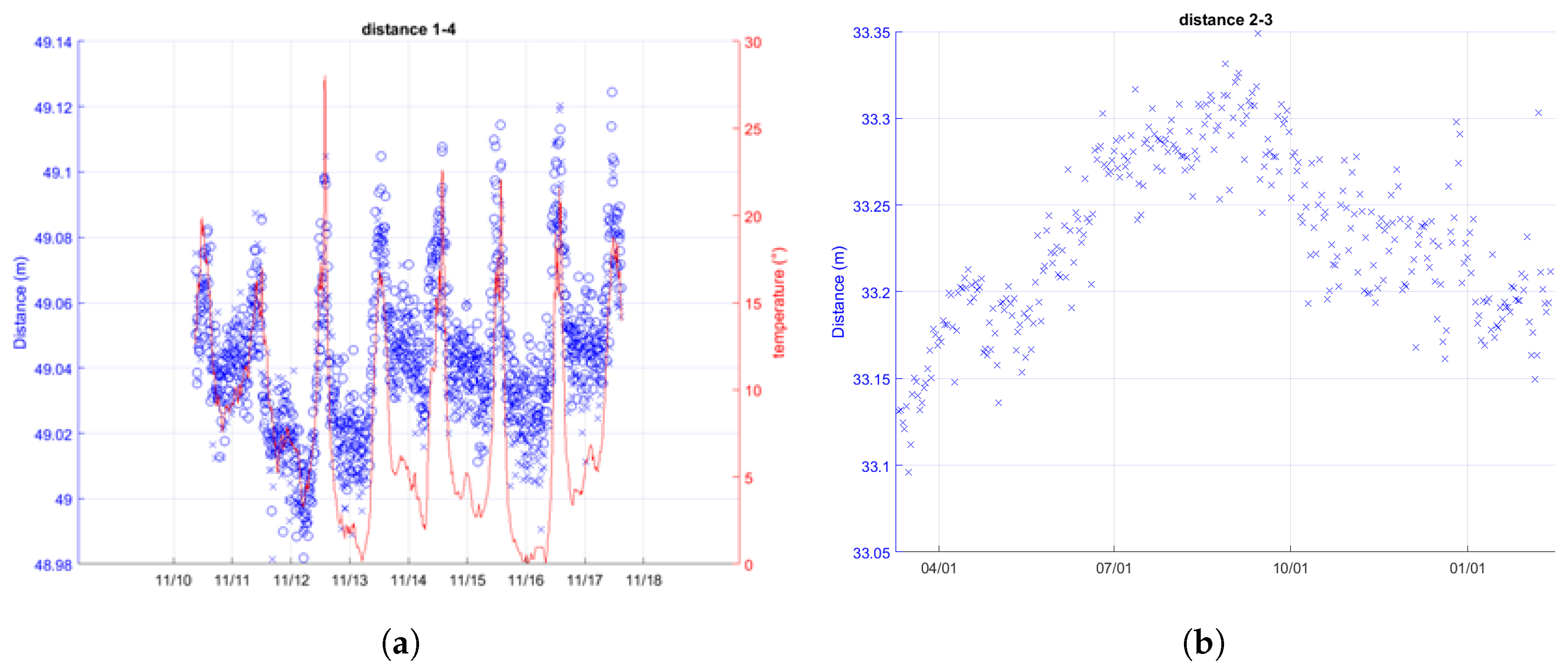
4.2.2. Temperature Effect
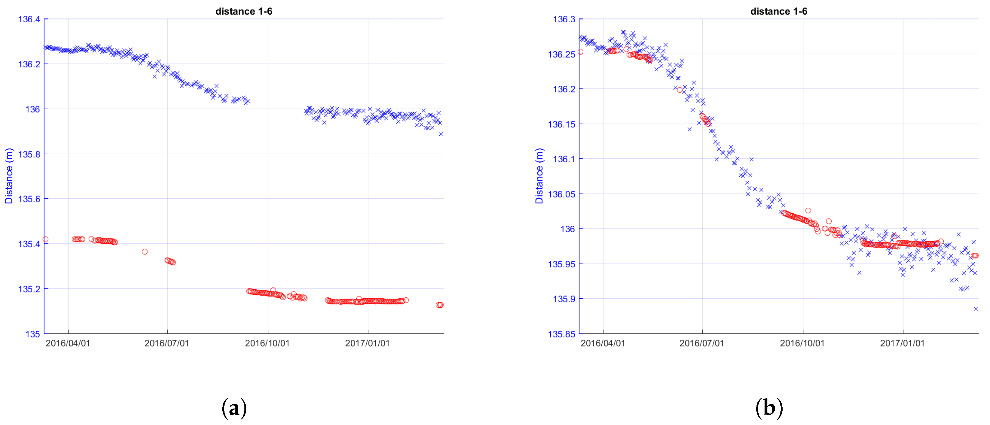
4.2.3. Long Distances Effect
5. Discussion
5.1. Benefits and Limits of Wi-GIM
- -
- Easy and quick installation. As described in Section 2.3, the Wi-GIM is characterized by an easy and fast deployment and set up. The system set up time is very low: only the MNs are required to be located in specific known positions of a stable area around the unstable and selected to be monitored one, where the SNs are displaced. As an example, a cluster of 10 slave sensors can be installed and configured in less than two hours.
- -
- Flexibility. Different kinds of landslide, subsidence cases or other ground deformations can be monitored by the Wi-GIM without requiring specific effort for the system adaptability.
- -
- Cost effective. Wi-GIM is characterized by an affordable cost, also making reasonable the monitoring of a large area.
- -
- Accuracy. The integrated technologies of Wi-GIM assure the accuracy needed for analyzing different kinds of ground movements. Obstacle avoidance. The nodes do not need to be in LOS in order to determine their position.
- -
- Scalability. Possibility to monitor movements on a lattice consisting of a large number of nodes.
- -
- 3D monitoring. Wi-GIM allows the 3D monitoring of the movements, also on a lattice consisting of a large number of nodes;
5.2. Considerations on the Factors of Influence in the UWB Ranging Accuracy
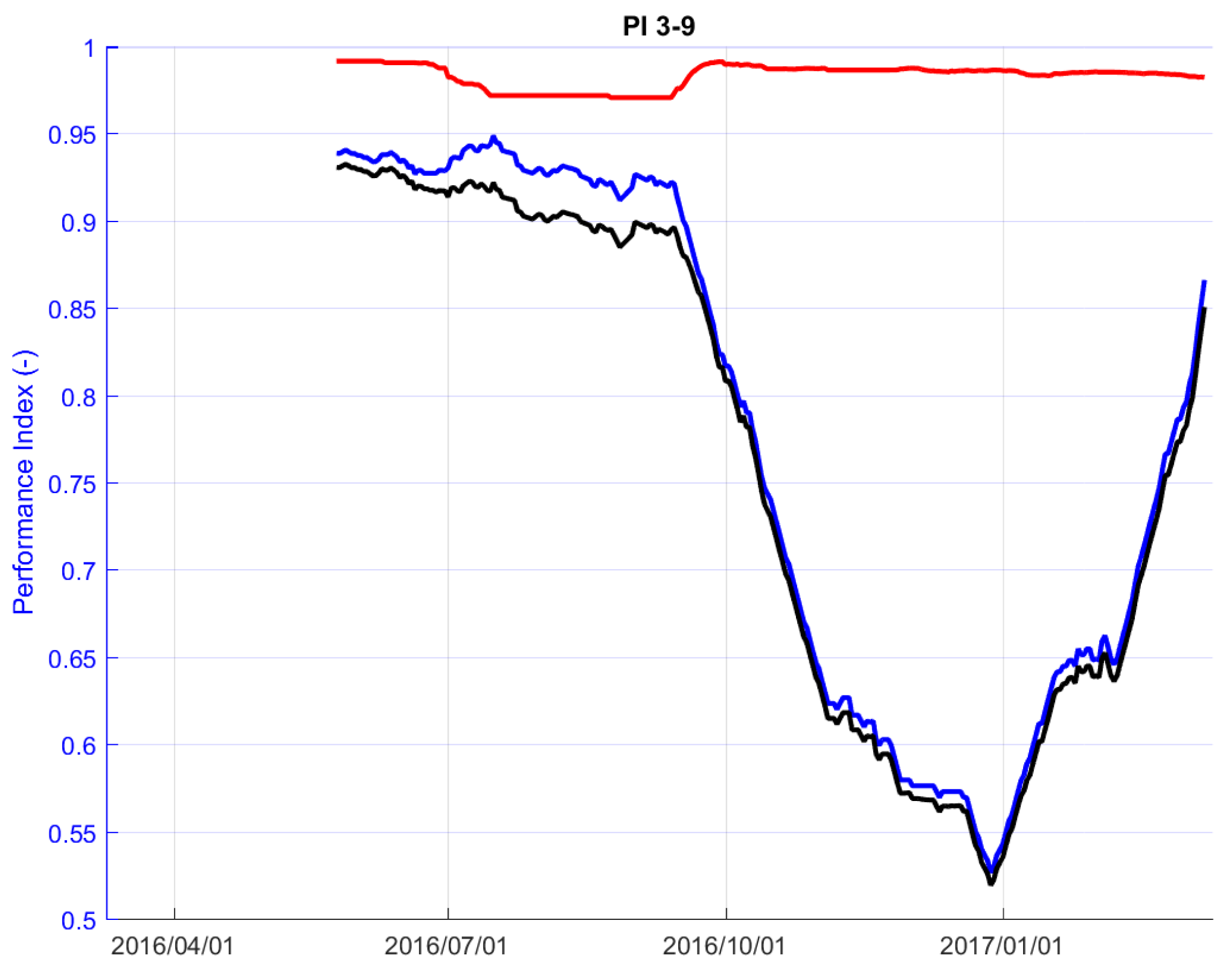
5.3. Performance Index
6. Conclusions
Author Contributions
Funding
Acknowledgments
Conflicts of Interest
References
- Casagli, N.; Frodella, W.; Morelli, S.; Tofani, T.; Ciampalini, A.; Intrieri, E.; Raspini, F.; Rossi, G.; Tanteri, L.; Lu, P. Spaceborne, UAV And Ground-Based Remote Sensing Techniques For Landslide Mapping, Monitoring And Early Warning. Geoenviron. Disasters 2017, 4, 9. [Google Scholar] [CrossRef]
- Intrieri, E.; Gigli, G.; Gracchi, T.; Nocentini, M.; Lombardi, L.; Mugnai, F.; Frodella, W.; Bertolini, G.; Carnevale, E.; Favalli, M.; et al. Application of an ultra-wide band sensor-free wireless network for ground monitoring. Eng. Geol. 2018, 238, 1–14. [Google Scholar] [CrossRef]
- Farina, P.; Leoni, L.; Babboni, F.; Coppi, F.; Mayer, L.; Ricci, P. IBIS-M, an innovative radar for monitoring slopes in open-pit mines. In Proceedings of the Slope Stability 2011: International Symposium on Rock Slope Stability in Open Pit Mining and Civil Engineering, Vancouver, BC, Canada, 18–21 September 2011. [Google Scholar]
- Read, J.; Stacey, P. Guidelines for Open Pit Slope Design; CSIRO Publishing: Clayton, Australia, 2009. [Google Scholar]
- Severin, J.; Eberhardt, E.; Leoni, L.; Fortin, S. Development and application of a pseudo-3D pit slope displacement map derived from ground-based radar. Eng. Geol. 2014, 181, 202–211. [Google Scholar] [CrossRef]
- Lombardi, L.; Nocentini, M.; Frodella, W.; Nolesini, T.; Bardi, F.; Intrieri, E.; Carlà, T.; Solari, L.; Dotta, G.; Ferrigno, F.; et al. The Calatabiano landslide (southern Italy): Preliminary GB-InSAR monitoring data and remote 3D mapping. Landslides 2017, 14, 685–696. [Google Scholar] [CrossRef]
- Giordan, D.; Allasia, P.; Manconi, A.; Baldo, M.; Santangelo, M.; Cardinali, M.; Corazza, A.; Albanese, V.; Lollino, G.; Guzzetti, F. Morphological and kinematic evolution of a large earthflow: The Montaguto landslide, southern Italy. Geomorphology 2013, 187, 61–79. [Google Scholar] [CrossRef]
- Mantovani, F.; Pasuto, A.; Silvano, S.; Zannoni, A. Collecting data to define future hazard scenarios of the Tessina landslide. Int. J. Appl. Earth Obs. Geoinf. 2000, 2, 33–40. [Google Scholar] [CrossRef]
- Rizzo, V.; Leggeri, M. Slope instability and sagging reactivation at Maratea (Potenza, Basilicata, Italy). Eng. Geol. 2004, 71, 181–198. [Google Scholar] [CrossRef]
- Petley, D.N.; Mantovani, F.; Bulmer, M.H.; Zannoni, A. The use of surface monitoring data for the interpretation of landslide movement patterns. Geomorphology 2005, 66, 133–147. [Google Scholar] [CrossRef]
- Gili, J.A.; Corominas, J.; Rius, J. Using global positioning system techniques in landslide monitoring. Eng. Geol. 2000, 55, 167–192. [Google Scholar] [CrossRef]
- Malet, J.P.; Maquaire, O.; Calais, E. The use of Global Positioning System techniques for the continuous monitoring of landslides: application to the Super-Sauze earthflow (Alpes-de-Haute-Provence, France). Geomorphology 2002, 43, 33–54. [Google Scholar] [CrossRef]
- Mora, P.; Baldi, P.; Casula, G.; Fabris, M.; Ghirotti, M.; Mazzini, E.; Pesci, A. Global Positioning Systems and digital photogrammetry for the monitoring of mass movements: Application to the Ca’di Malta landslide (northern Apennines, Italy). Eng. Geol. 2003, 68, 103–121. [Google Scholar] [CrossRef]
- Squarzoni, C.; Delacourt, C.; Allemand, P. Differential single-frequency GPS monitoring of the La Valette landslide (French Alps). Eng. Geol. 2005, 79, 215–229. [Google Scholar] [CrossRef]
- Teja, G.N.L.R.; Harish, V.K.R.; Khan, D.N.M.; Krishna, R.B.; Singh, R.; Chaudhary, S. Land Slide detection and monitoring system using wireless sensor networks (WSN). In Proceedings of the 2014 IEEE International Advance Computing Conference (IACC), Gurgaon, New Delhi, India, 21–22 February 2014; pp. 149–154. [Google Scholar]
- Sheth, A.; Tejaswi, K.; Mehta, P.; Parekh, C.; Bansal, R.; Merchant, S.; Singh, T.; Desai, U.B.; Thekkath, C.A.; Toyama, K. Senslide: A sensor network based landslide prediction system. In Proceedings of the 3rd International Conference on Embedded Networked Sensor Systems, San Diego, CA, USA, 2–4 November 2005; pp. 280–281. [Google Scholar]
- Mehta, P.; Chander, D.; Shahim, M.; Tejaswi, K.; Merchant, S.N.; Desai, U.B. Distributed detection for landslide prediction using wireless sensor network. In Proceedings of the First International Global Information Infrastructure Symposium, Marrakech, Morocco, 2–6 July 2007. [Google Scholar]
- Rosi, A.; Berti, M.; Bicocchi, N.; Castelli, G.; Corsini, A.; Mamei, M.; Zambonelli, F. Landslide monitoring with sensor networks: Experiences and lessons learnt from a real-world deployment. Int. J. Sens. Netw. 2011, 10, 111–122. [Google Scholar] [CrossRef]
- Dai, K.; Chen, S. Strong ground movement induced by mining activities and its effect on power transmission structures. Min. Sci. Technol. 2009, 19, 563–568. [Google Scholar] [CrossRef]
- Wi-GIM Project Official Web Site. Available online: http://www.life-wigim.eu/ (accessed on 31 August 2018).
- Win, M.Z.; Dardari, D.; Molisch, A.F.; Wiesbeck, W.; Zhang, J. History and Applications of UWB. Proc. IEEE 2009, 97, 198–204. [Google Scholar] [CrossRef]
- Win, M.Z.; Scholtz, R.A. Impulse radio: How it works. IEEE Commun. Lett. 1998, 2, 36–38. [Google Scholar] [CrossRef]
- Groves, P.D. Principles of GNSS, Inertial, and Multisensor Integrated Navigation Systems, 2nd ed.; Artech House: Norwood, MA, USA, 2013. [Google Scholar]
- Bertolini, G. Large earth flows in Emilia-Romagna (Northern Apennines, Italy): Origin, reactivation and possible hazard assessment strategies [Große Schuttströme in Emilia-Romagna (Nördlicher Apennin, Italien): Ursache, Reaktivierung und mögliche Strategien zur Gefahrenbeurteilung]. Zeitschrift der Deutschen Gesellschaft für Geowissenschaften 2010, 161, 139–162. [Google Scholar]
- Bertolini, G.; Fioroni, C. Large Reactivated Earth Flows in the Northern Apennines (Italy): An Overview. In Landslide Science and Practice; Springer: Berlin/Heidelberg, Germany, 2013; pp. 51–58. [Google Scholar]
- FMCW Radar Sensors. Application Notes. 2011. Available online: https://www.siversima.com/wp-content/ uploads/FMCW-Radar-App-Note.pdf (accessed on 30 August 2018).
- Falsi, C.; Dardari, D.; Mucchi, L.; Win, M.Z. Range estimation in UWB realistic environments. In Proceedings of the IEEE International Conference on Communications (ICC), Istanbul, Turkey, 11–15 June 2006; pp. 5692–5697. [Google Scholar]
- Monserrat, O.; Crosetto, M.; Luzi, G. A review of ground-based SAR interferometry for deformation measurement. ISPRS J. Photogramm. Remote Sens. 2014, 93, 40–48. [Google Scholar] [CrossRef]
- Del Ventisette, C.; Gigli, G.; Tofani, V.; Lu, P.; Casagli, N. Radar Technologies for Landslide Detection, Monitoring, Early Warning and Emergency Management. In Modern Technologies for Landslide Monitoring and Prediction; Scaioni, M., Ed.; Springer Natural Hazards; Springer: Berlin/Heidelberg, Germay, 2015. [Google Scholar]
- Molisch, A. Wireless Communications, 2nd ed.; Wiley: Hoboken, NJ, USA, 2011. [Google Scholar]
- Decawave. Decawave DWM1000 Datasheet. 2018. Available online: https://www.decawave.com/sites/default/files/resources/DWM1000-Datasheet-V1.6.pdf (accessed on 30 August 2018).
- Decawave. Decawave Application Note APS011. 2018. Available online: https://www.decawave.com/sites/default/files/resources/aps011_sources_of_error_in_twr.pdf (accessed on 30 August 2018).


| Component/Module | Function | MN | SN |
|---|---|---|---|
| Micro-controller | ARM Cortex M3 micro-controller. | X | X |
| Battery | A 12 V, 7.2 Ah lead acid battery for node power supply. | X | X |
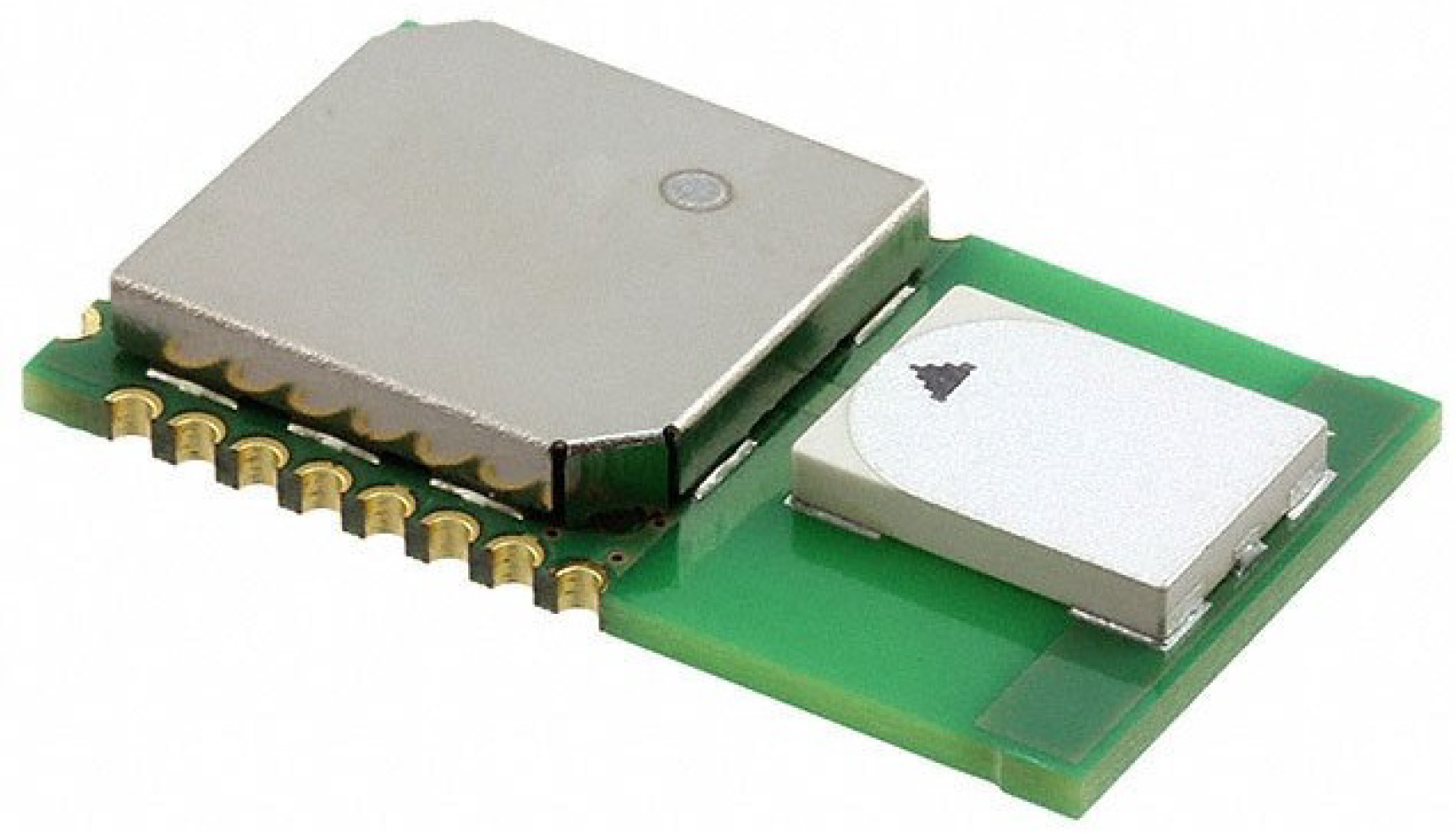
| UWB | Decawave Sensor DWM1000 Module (2017a) for communications and ranging. | X | X |
| SD memory card | Storage of the IDs of SNs and the number of hops to reach them. | X | |
| GPS | Time reference signal required for slave coordination. | X | X(*) |
| GSM/GPRS/3G | Long-range communication modules for data transmission to the remote server. | X |
| Cluster No. | Nodes | Installation (yyyy/mm/dd) | Removal (yyyy/mm/dd) | Test Objective |
|---|---|---|---|---|
| 1 | 1 MN and 3 SNs | 2016/10/13 | 2017/02/06 | Inter-visibility between couples of |
| nodes of the same network | ||||
| 2 | 1 MN and 3 SNs | 2016/11/11 | 2017/01/20 | Temperature influence on |
| the ranging measurement | ||||
| 3 | 1 MN and 1 SN | 2016/12/12 | 2016/12/27 | System behaviour in case |
| of obstacles between nodes | ||||
| 4 | 1 MN and 1 SN | 2017/01/03 | 2017/02/01 | System behaviour in case |
| of obstacles between nodes | ||||
| 5 | 1 MN and 1 SN | 2017/01/20 | 2017/02/06 | System behaviour in case |
| of obstacles between nodes | ||||
| 6 | 1 MN and 1 SN | 2017/02/01 | 2017/02/16 | System behaviour in case |
| of obstacles between nodes |
| Technology | Maximum Inter-Node Distance (m) | Precision (m) | Filters | Notes |
|---|---|---|---|---|
| UWB | 110 | 0.1–0.2 | - | LOS |
| 60 | 0.07–0.1 | Outlier filtering Statistic filtering | Antenna at 1 m to the ground | |
| 60 | 0.02–0.03 | Outlier filtering, statistic filtering, | Antenna at 1 m to the ground | |
| temperature compensation | ||||
| CWR | 60 | 0.07–0.1 | Frequency | - |
| 60 | 0.01 | Frequency + Phase + MUltiple SIgnal | Vertical shift higher than 12 cm | |
| Classification (MUSIC) Algorithm | needed to discriminate the signal | |||
| 10 | 0.007–0.009 | Frequency + Phase | Normal corner reflector |
| Condition | Real Distance (m) | Distance Mean (m) | Standard Dev. (m) | Error (m) |
|---|---|---|---|---|
| LOS | 0.37 | 0.364 | 0.022 | 0.006 |
| Indoor | 9.7 | 9.736 | 0.020 | 0.036 |
| 30.32 | 30.278 | 0.026 | 0.042 | |
| LOS | 2.57 | 2.623 | 0.022 | 0.053 |
| Outdoor | 3.37 | 3.329 | 0.017 | 0.041 |
| 25.32 | 25.391 | 0.0222 | 0.071 | |
| NLOS | 0.39 | 0.385 | 0.029 | 0.005 |
| Indoor | 5.42 | 5.486 | 0.031 | 0.066 |
| 29.83 | 29.789 | 0.028 | 0.041 |
| Cluster No. | Nodes | Distance (m) | Trend Line Slope (m) |
|---|---|---|---|
| 1–4 | 49 | 0.0029 | |
| 1 | 3–4 | 38 | 0.0025 |
| 1–3 | 22 | 0.0030 | |
| 1–4 | 3 | 0.0070 | |
| 2 | 3–4 | 67 | 0.0060 |
| 1–3 | 67 | 0.0063 |
| Cluster No. | Pair of Nodes | Distance (m) | Standard Deviation (%) |
|---|---|---|---|
| 3–4 | 15 | 4.7 | |
| 1 | 1–3 | 70 | 3.5 |
| 1–7 | 132 | 2.6 | |
| 2–11 | 37 | 3.6 | |
| 2 | 1–2 | 80 | 3.0 |
| 5–12 | 130 | 3.4 |
| Feature | Wi-GIM | RTS | GB-InSAR |
|---|---|---|---|
| Environmental impact | 3 | 4 | 4 |
| Installation effort | 5 | 3 | 4 |
| Influence of rain | 4 | 3 | 1 |
| Influence of snow | 4 | 3 | 4 |
| Completeness of information | 4 | 5 | 5 |
| Case | Monitored Area (m) | Wi-GIM Cost (€) | RTS Cost (€) | GB-InSAR Cost (€) |
|---|---|---|---|---|
| 1 | 500 | 2820 | 14,750 | 58,100 |
| 2 | 100,000 | 5220 | 18,150 | 58,100 |
| Feature | Wi-GIM | RTS | GB-InSAR |
|---|---|---|---|
| Durability | 2 | 3 | 5 |
| Precision | 2 | 4 | 5 |
| Maximum range | 2 | 5 | 5 |
© 2018 by the authors. Licensee MDPI, Basel, Switzerland. This article is an open access article distributed under the terms and conditions of the Creative Commons Attribution (CC BY) license (http://creativecommons.org/licenses/by/4.0/).
Share and Cite
Mucchi, L.; Jayousi, S.; Martinelli, A.; Caputo, S.; Intrieri, E.; Gigli, G.; Gracchi, T.; Mugnai, F.; Favalli, M.; Fornaciai, A.; et al. A Flexible Wireless Sensor Network Based on Ultra-Wide Band Technology for Ground Instability Monitoring. Sensors 2018, 18, 2948. https://doi.org/10.3390/s18092948
Mucchi L, Jayousi S, Martinelli A, Caputo S, Intrieri E, Gigli G, Gracchi T, Mugnai F, Favalli M, Fornaciai A, et al. A Flexible Wireless Sensor Network Based on Ultra-Wide Band Technology for Ground Instability Monitoring. Sensors. 2018; 18(9):2948. https://doi.org/10.3390/s18092948
Chicago/Turabian StyleMucchi, Lorenzo, Sara Jayousi, Alessio Martinelli, Stefano Caputo, Emanuele Intrieri, Giovanni Gigli, Teresa Gracchi, Francesco Mugnai, Massimiliano Favalli, Alessandro Fornaciai, and et al. 2018. "A Flexible Wireless Sensor Network Based on Ultra-Wide Band Technology for Ground Instability Monitoring" Sensors 18, no. 9: 2948. https://doi.org/10.3390/s18092948
APA StyleMucchi, L., Jayousi, S., Martinelli, A., Caputo, S., Intrieri, E., Gigli, G., Gracchi, T., Mugnai, F., Favalli, M., Fornaciai, A., & Nannipieri, L. (2018). A Flexible Wireless Sensor Network Based on Ultra-Wide Band Technology for Ground Instability Monitoring. Sensors, 18(9), 2948. https://doi.org/10.3390/s18092948