Joint Source and Channel Rate Allocation over Noisy Channels in a Vehicle Tracking Multimedia Internet of Things System


Abstract
1. Introduction
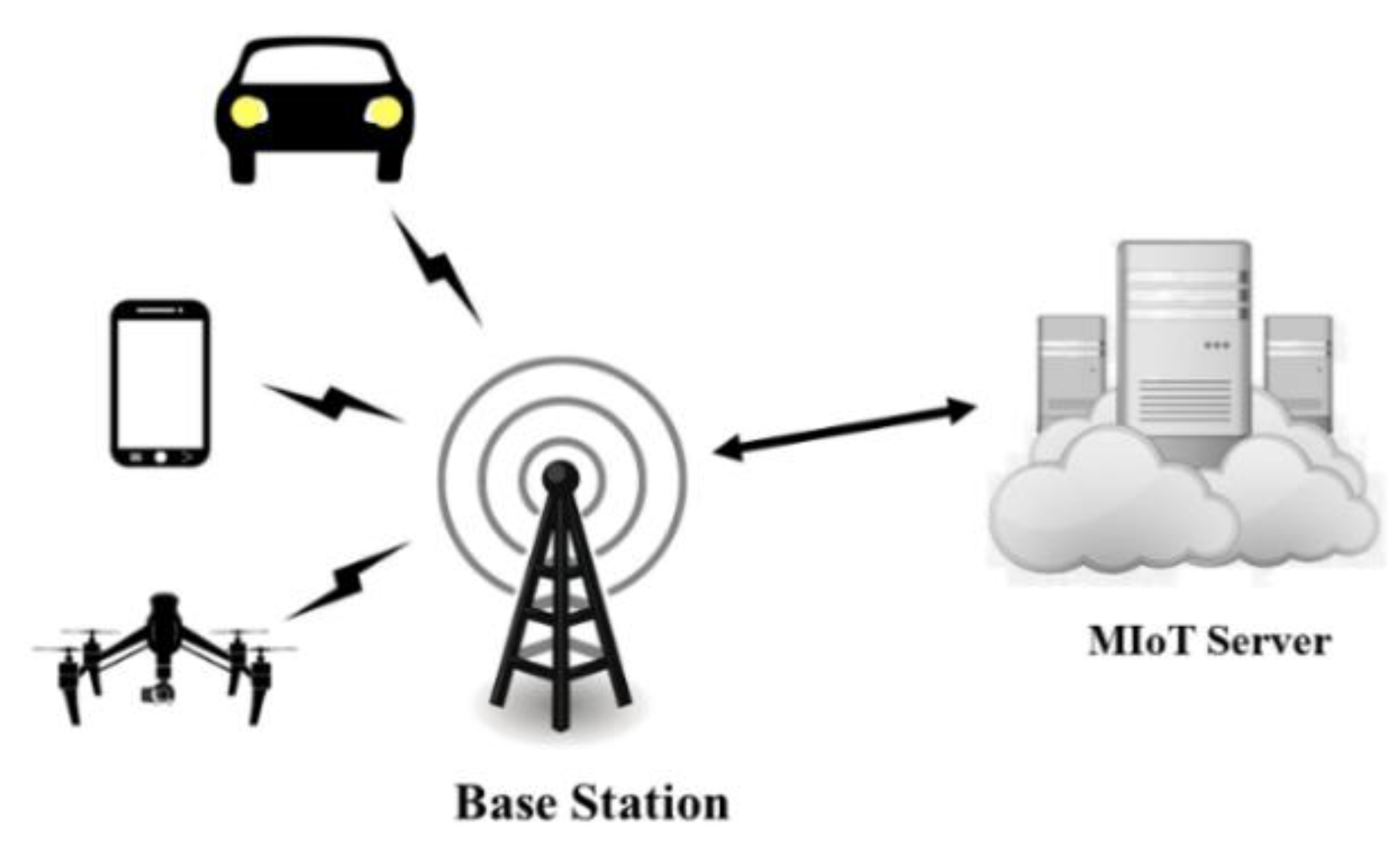
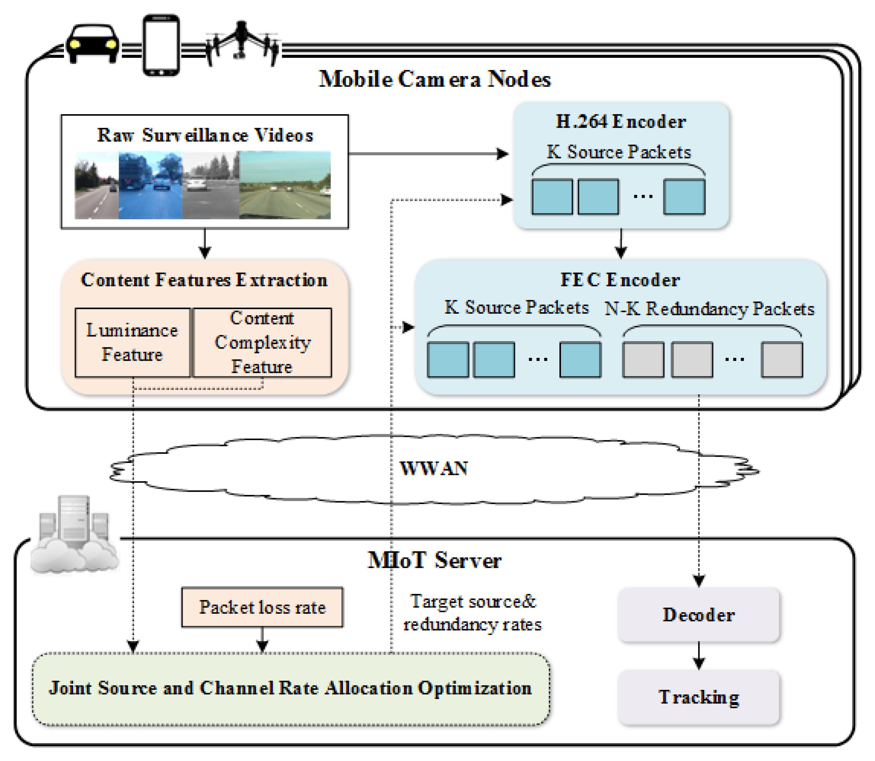
2. Scenarios and Structure of MIoT System for Vehicle Tracking
3. Content-Aware Tracking Precision Prediction Model
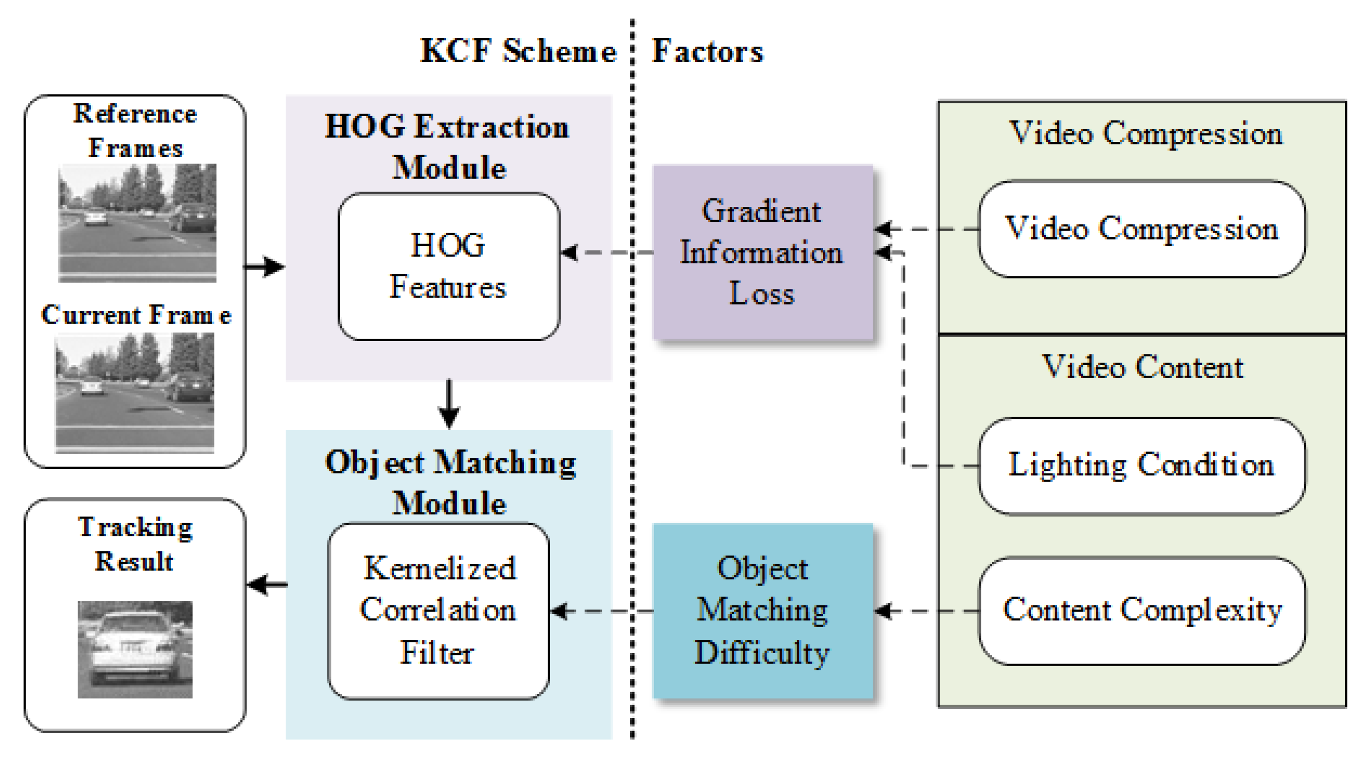
3.1. Factors Impact on KCF Tracking Scheme
3.2. Model Features Extraction and Analysis
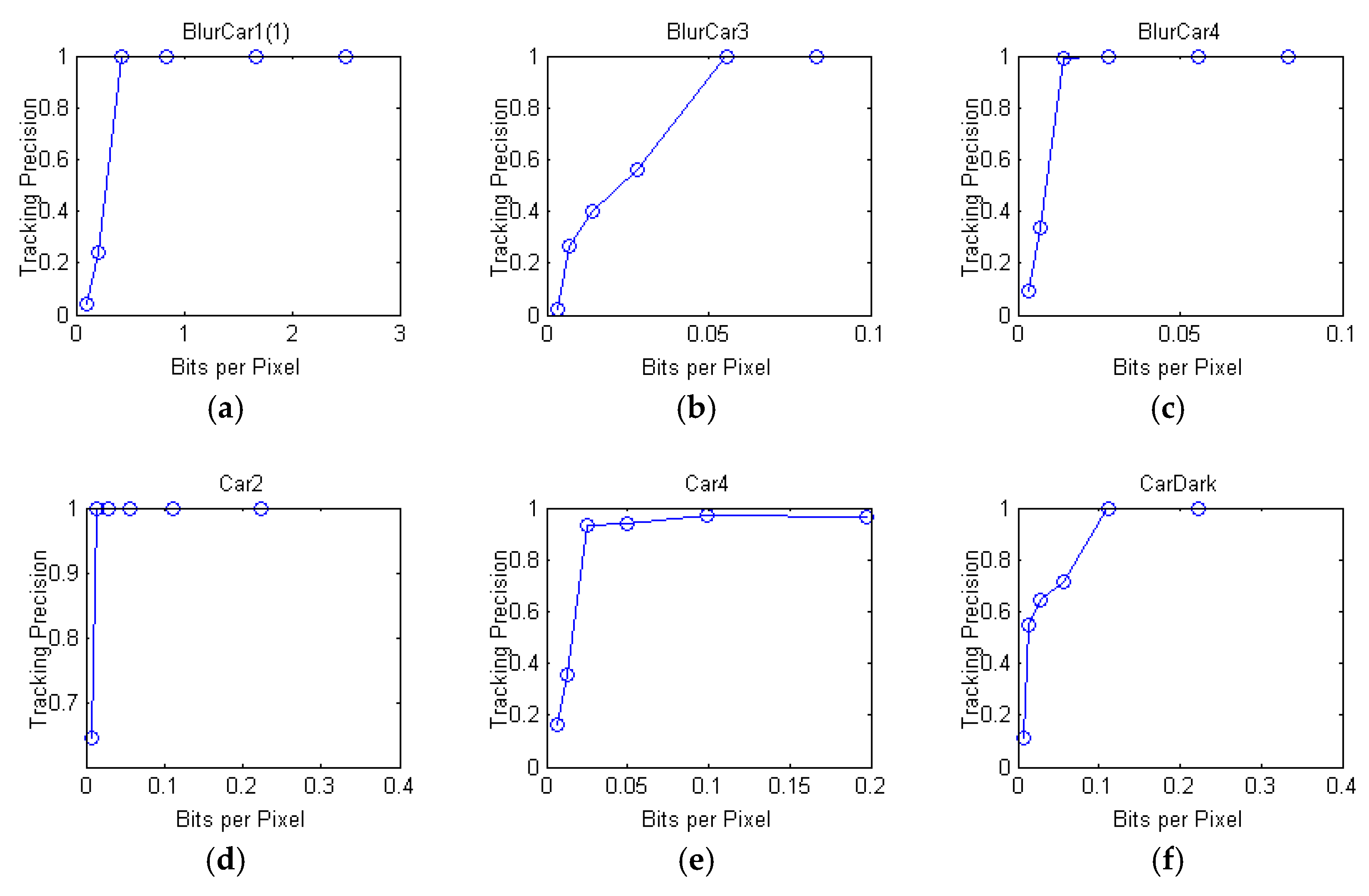
3.2.1. Bits per Pixel
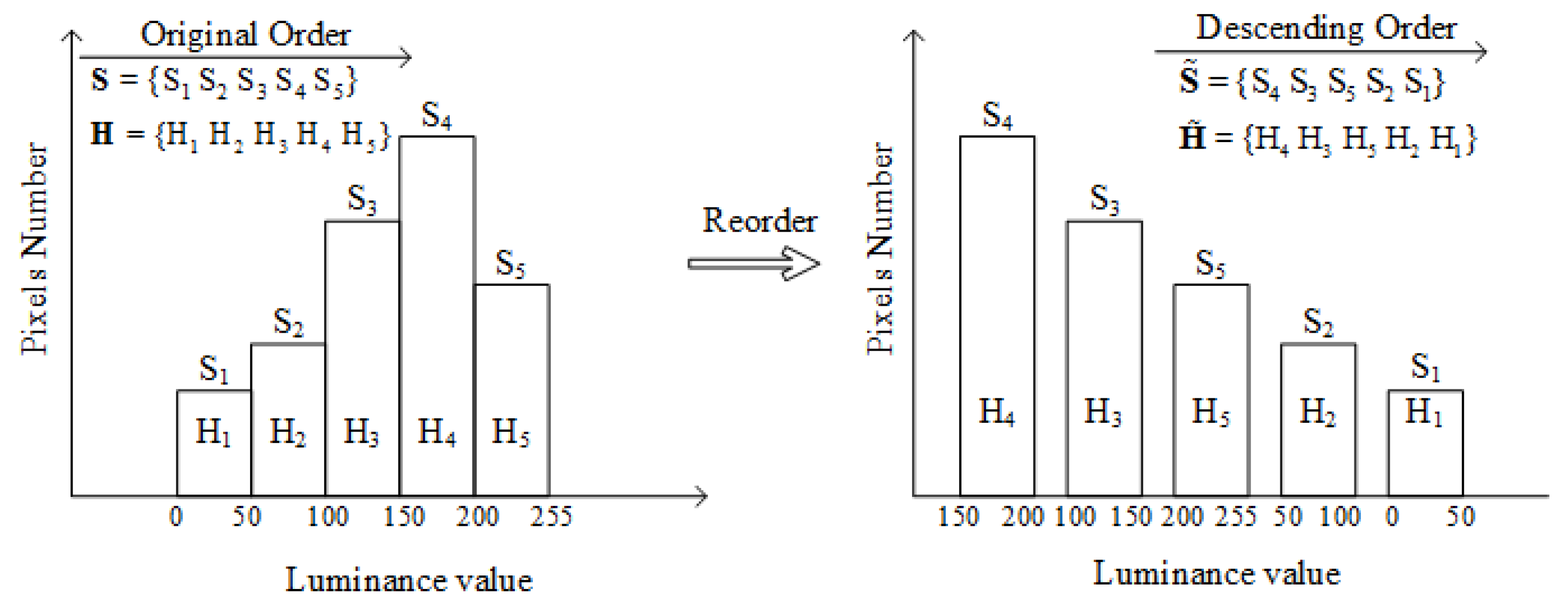
3.2.2. Video Luminance Level
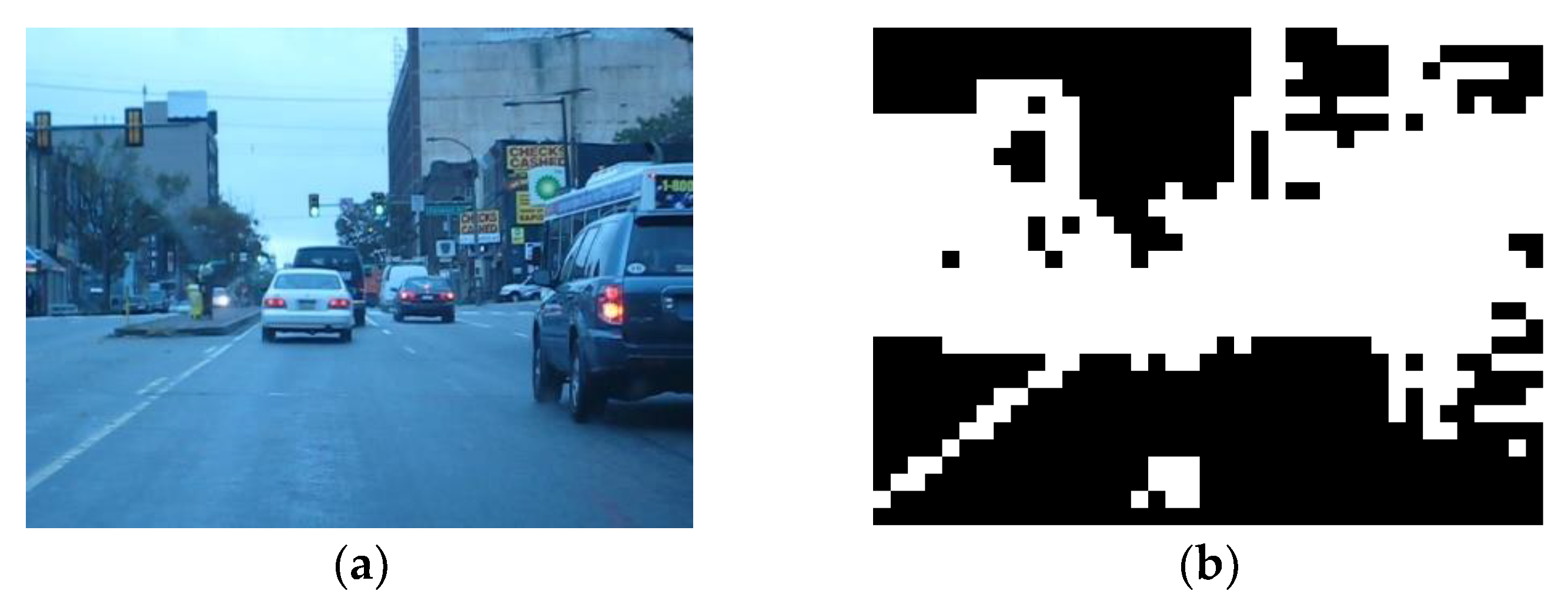
3.2.3. Video Adjacent Block Difference
3.3. Model Establishment
4. Proposed Joint Source and Channel Rate Allocation Scheme
5. Simulation and Performance Comparison
5.1. Simulation Settings
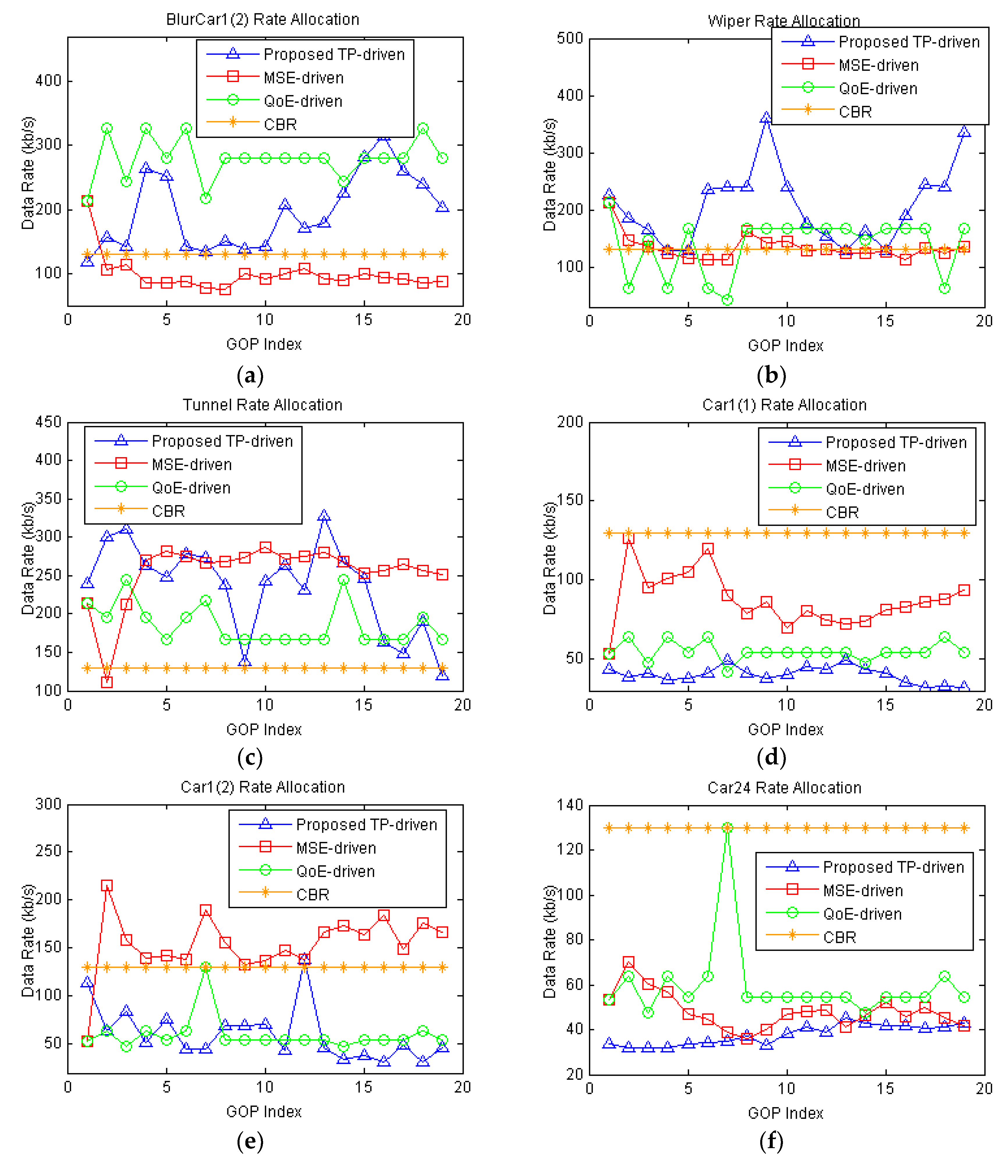
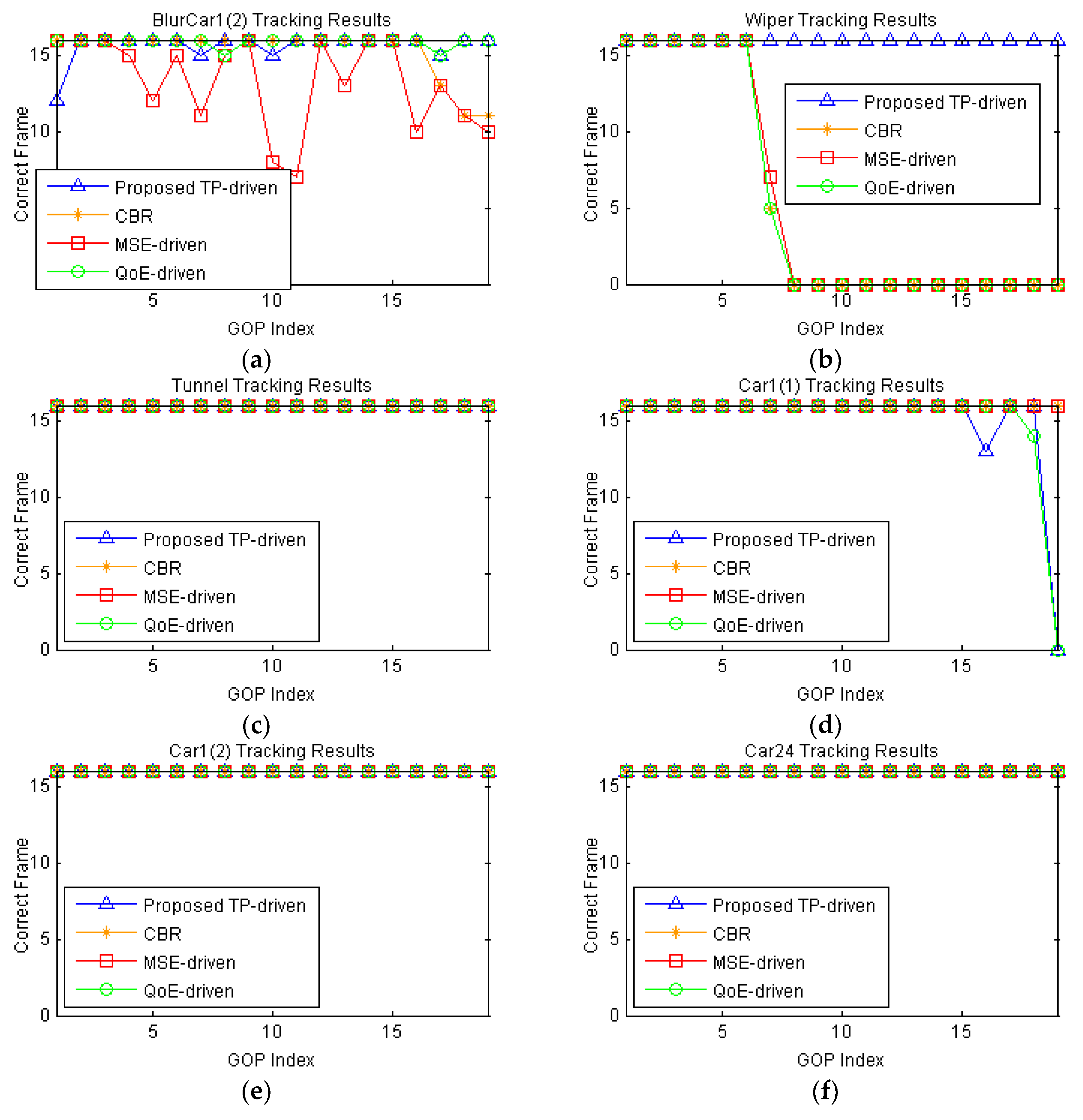
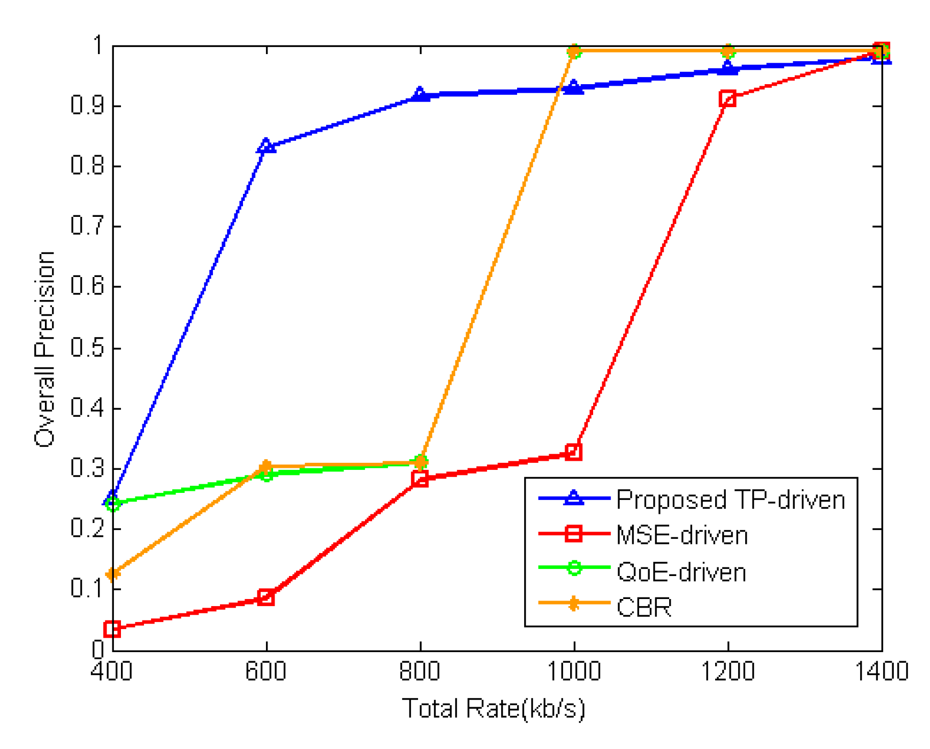
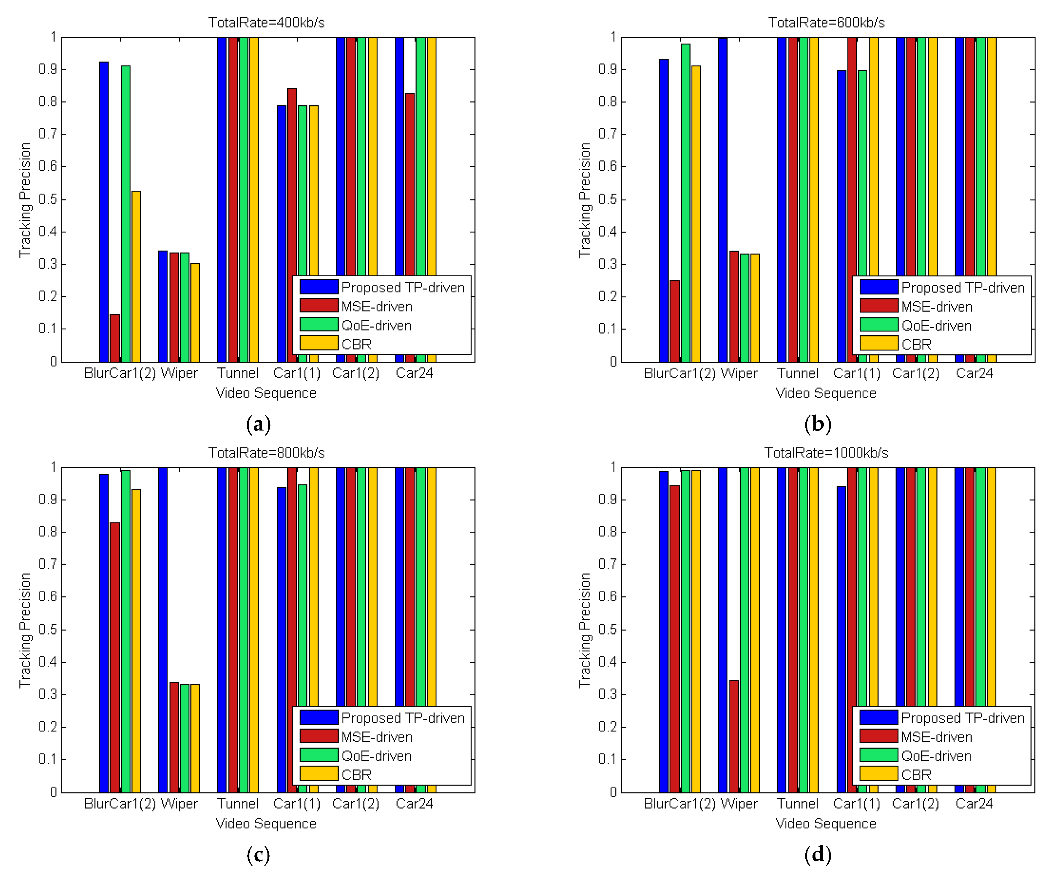
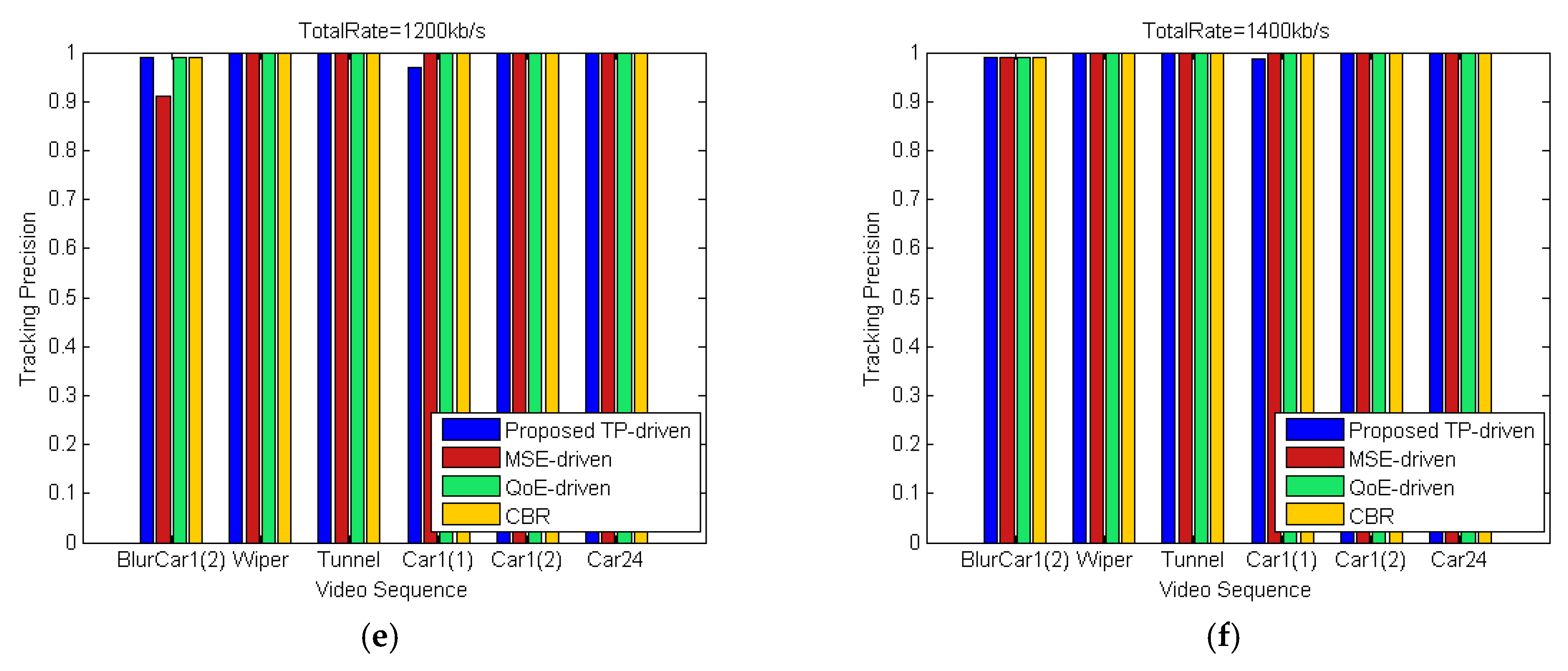
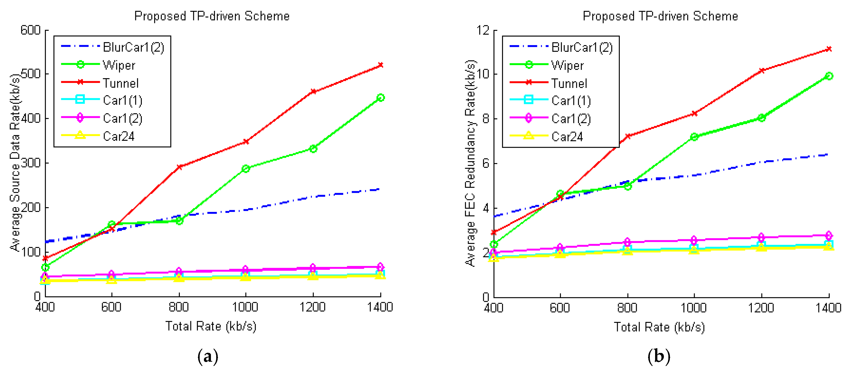
5.2. Simulation Results and Discussion
6. Conclusions
Author Contributions
Funding
Conflicts of Interest
References
- ITU-T Recommendation, Y. 2060 Overview of the Internet of Things. Available online: http://www.itu.int/rec/T-REC-Y.2060/en (accessed on 29 August 2018).
- Floris, A.; Atzori, L. Managing the quality of experience in the multimedia internet of things: A layered-based approach. Sensors 2016, 16, 2057. [Google Scholar] [CrossRef] [PubMed]
- Huang, Q.; Wang, W.; Zhang, Q. Your glasses know your diet: Dietary monitoring using electromyography sensors. IEEE Int. Things J. 2017, 4, 705–712. [Google Scholar] [CrossRef]
- Catarinucci, L.; Donno, D.D.; Mainetti, L. An IoT—aware architecture for smart healthcare systems. IEEE Int. Things J. 2015, 2, 515–526. [Google Scholar] [CrossRef]
- Lobaccaro, G.; Carlucci, S.; Löfström, E. A review of systems and technologies for smart homes and smart grids. Energies 2016, 9, 348. [Google Scholar] [CrossRef]
- Choi, H.S.; Rhee, W.S. IoT-based user-driven service modeling environment for a smart space management system. Sensors 2014, 14, 22039. [Google Scholar] [CrossRef] [PubMed]
- Masek, P.; Masek, J.; Frantik, P. A Harmonized perspective on transportation management in smart cities: The novel iot-driven environment for road traffic modeling. Sensors 2016, 16, 1872. [Google Scholar] [CrossRef] [PubMed]
- Sutar, S.H.; Koul, R.; Suryavanshi, R. Integration of smart phone and IOT for development of smart public transportation system. In Proceedings of the IEEE International Conference on Internet of Things and Applications, Pune, India, 22–24 January 2016; pp. 73–78. [Google Scholar]
- Kokkonis, G.; Psannis, K.E.; Roumeliotis, M. Real-time wireless multisensory smart surveillance with 3D-HEVC streams for internet-of-things (IoT). J. Supercomput. 2017, 73, 1–19. [Google Scholar] [CrossRef]
- Wang, M.; Cheng, B.; Yuen, C. Joint coding-transmission optimization for a video surveillance system with multiple cameras. IEEE Trans. Multimedia 2018, 20, 620–633. [Google Scholar] [CrossRef]
- Cajote, R.D.; Ruangsang, W.; Aramvith, S. Wireless video transmission over MIMO-OFDM using background modeling for video surveillance applications. In Proceedings of the IEEE International Symposium on Communications and Information Technologies, Nara, Japan, 7–9 October 2015; pp. 237–240. [Google Scholar]
- Li, F.; Fu, S.; Liu, Z.; Qian, X. A cost-constrained video quality satisfaction study on mobile devices. IEEE Trans. Multimedia 2018, 20, 1154–1168. [Google Scholar] [CrossRef]
- Liu, Z.; Cheung, G.; Ji, Y. Optimizing distributed source coding for interactive multiview video streaming over lossy networks. IEEE Trans. Circuits Syst. Video Technol. 2013, 23, 1781–1794. [Google Scholar] [CrossRef]
- Feng, J.; Liu, Z.; Ji, Y. Wireless channel loss analysis—A case study using wifi-direct. In Proceedings of the International Wireless Communications and Mobile Computing Conference, Nicosia, Cyprus, 4–8 August 2014; pp. 244–249. [Google Scholar]
- Liu, Z.; Ishihara, S.; Cui, Y.; Ji, Y.; Tanaka, Y. JET: Joint source and channel coding for error resilient virtual reality video wireless transmission. Signal Process. 2018, 147, 154–162. [Google Scholar] [CrossRef]
- Bilal, M.; Khan, A.; Khan, M.U.K. A Low Complexity Pedestrian Detection Framework for Smart Video Surveillance Systems. IEEE Trans. Circuits Syst. Video Technol. 2017, 27, 2260–2273. [Google Scholar] [CrossRef]
- Li, F.; Zhang, S.; Qiao, X. Scene-Aware Adaptive Updating for Visual Tracking via Correlation Filters. Sensors 2017, 17, 2626. [Google Scholar] [CrossRef] [PubMed]
- Tran, N.N.; Long, H.P.; Tran, H.M. Scene recognition in traffic surveillance system using neural network and probabilistic model. In Proceedings of the IEEE International Conference on System Science and Engineering, Ho Chi Minh City, Vietnam, 21–23 July 2017; pp. 226–230. [Google Scholar]
- Jung, H.; Choi, M.K.; Jung, J. ResNet-based vehicle classification and localization in traffic surveillance systems. In Proceedings of the IEEE Computer Vision and Pattern Recognition Workshops, Honolulu, HI, USA, 21–26 July 2017; pp. 934–940. [Google Scholar]
- Lee, K.H.; Hwang, J.N.; Chen, S.I. Model-based vehicle localization based on 3-d constrained multiple-kernel tracking. IEEE Trans. Circuits Syst. Video Technol. 2015, 25, 38–50. [Google Scholar] [CrossRef]
- Felzenszwalb, P.F.; Girshick, R.B.; McAllester, D. Object detection with discriminatively trained part-based models. IEEE Trans. Pattern Anal. Mach. Intell. 2010, 32, 1627–1645. [Google Scholar] [CrossRef] [PubMed]
- Ren, S.; He, K.; Girshick, R. Faster R-CNN: Towards real-time object detection with region proposal networks. IEEE Trans. Pattern Anal. Mach. Intell. 2015, 39, 1137–1149. [Google Scholar] [CrossRef] [PubMed]
- Bolme, D.S.; Beveridge, J.R.; Draper, B.A. Visual object tracking using adaptive correlation filters. In Proceedings of the IEEE Computer Vision and Pattern Recognition, San Francisco, CA, USA, 13–18 June 2010; pp. 2544–2550. [Google Scholar]
- Henriques, J.F.; Rui, C.; Martins, P. Exploiting the circulant structure of tracking-by-detection with kernels. In Proceedings of the European Conference on Computer Vision, Florence, Italy, 7–13 October 2012; pp. 702–715. [Google Scholar]
- Henriques, J.F.; Rui, C.; Martins, P. High-speed tracking with kernelized correlation filters. IEEE Trans. Pattern Anal. Mach. Intell. 2015, 37, 583–596. [Google Scholar] [CrossRef] [PubMed]
- Girod, B.; Chandrasekhar, V.; Chen, D.M. Mobile visual search. IEEE Signal Process. Mag. 2011, 28, 61–76. [Google Scholar] [CrossRef]
- Redondi, A.; Cesana, M.; Tagliasacchi, M. Rate-accuracy optimization in visual wireless sensor networks. In Proceedings of the IEEE International Conference on Image Processing, Orlando, FL, USA, 30 September–3 October 2012; pp. 1105–1108. [Google Scholar]
- Lee, K.H.; Hwang, J.N. On-road pedestrian tracking across multiple driving recorders. IEEE Trans. Multimedia 2015, 17, 1429–1438. [Google Scholar] [CrossRef]
- Milani, S.; Bernardini, R.; Rinaldo, R. A saliency-based rate control for people detection in video. In Proceedings of the IEEE International Conference on Acoustics, Speech and Signal Processing, Vancouver, BC, Canada, 26–31 May 2013; pp. 2016–2020. [Google Scholar]
- Kong, L.; Dai, R. Object-detection-based video compression for wireless surveillance systems. IEEE Multimedia 2017, 24, 76–85. [Google Scholar] [CrossRef]
- Chen, X.; Hwang, J.N.; Lee, K.H.; de Queiroz, R.L. Quality-of-content (QoC)-driven rate allocation for video analysis in mobile surveillance networks. In Proceedings of the IEEE International Workshop on Multimedia Signal Processing, Xiamen, China, 19–21 October 2015; pp. 1–6. [Google Scholar]
- Chen, X.; Hwang, J.N.; Meng, D. A Quality-of-content-based joint source and channel coding for human detections in a mobile surveillance cloud. IEEE Trans. Circuits Syst. Video Technol. 2017, 27, 19–31. [Google Scholar] [CrossRef]
- Wei, H.; Gitli, R.D. Two-hop-relay architecture for next-generation WWAN/WLAN integration. IEEE Wirel. Commun. 2004, 11, 24–30. [Google Scholar] [CrossRef]
- Shokrollahi, A. Raptor codes. IEEE Trans. Inf. Theory 2006, 52, 2551–2567. [Google Scholar] [CrossRef]
- Wright, S.; Jones, S.; Lee, C. Guest Editorial-IPTV systems, standards and architectures: Part II. IEEE Commun. Mag. 2008, 46, 92–93. [Google Scholar] [CrossRef]
- Wu, J.; Shang, Y.; Huang, J.; Zhang, X.; Cheng, B.; Chen, J. Joint source-channel coding and optimization for mobile video streaming in heterogeneous wireless networks. EURASIP J. Wirel. Commun. Netw. 2013, 2013, 283. [Google Scholar] [CrossRef]
- Wu, Y.; Lim, J.; Yang, M.H. Online object tracking: A benchmark. In Proceedings of the IEEE Conference on Computer Vision and Pattern Recognition, Portland, OR, USA, 23–28 June 2013; pp. 2411–2418. [Google Scholar]
- Grant, M.; Boyd, S. CVX: MATLAB Software for Disciplined Convex Programming. Available online: http://cvxr.com/cvx (accessed on 3 August 2018).
- Kristan, M.; Leonardis, A.; Matas, J.; Felsberg, M.; Pflugfelder, R.; Čehovin, L.; Vojír̃, T.; Häger, G.; Lukežič, A.; Fernández, G.; et al. The visual object tracking vot2016 challenge results. In Proceedings of the European Conference on Computer Vision, Amsterdam, The Netherlands, 8–16 October 2016; pp. 191–217. [Google Scholar]
- Huang, Y.-H.; Ou, T.-S.; Su, P.-Y. Perceptual rate-distortion optimization using structural similarity index as quality metric. IEEE Trans. Circuits Syst. Video Technol. 2010, 20, 1614–1624. [Google Scholar] [CrossRef]
- Khan, A.; Sun, L.; Ifeachor, E. QoE Prediction Model and its Application in Video Quality Adaptation Over UMTS Networks. IEEE Trans. Multimedia 2012, 14, 431–442. [Google Scholar] [CrossRef]


| Video | Resolution | Bitrate(kb/s) | |||||
|---|---|---|---|---|---|---|---|
| BlurCar1(1) | 640 × 480 | 32 | 64 | 128 | 256 | 512 | 768 |
| BlurCar3 | 640 × 480 | 32 | 64 | 128 | 256 | 512 | 768 |
| BlurCar4 | 640 × 480 | 32 | 64 | 128 | 256 | 512 | 768 |
| Car2 | 320 × 240 | 16 | 32 | 64 | 128 | 256 | 512 |
| Car4 | 360 × 240 | 16 | 32 | 64 | 128 | 256 | 512 |
| CarDark | 320 × 240 | 16 | 32 | 64 | 128 | 256 | 512 |
| a1 | a2 | a3 | a4 |
| 12.661 | 7.034 | 200.560 | |
| a5 | a6 | a7 | a8 |
| 0.010 | 0.900 | 6.150 | 137.000 |
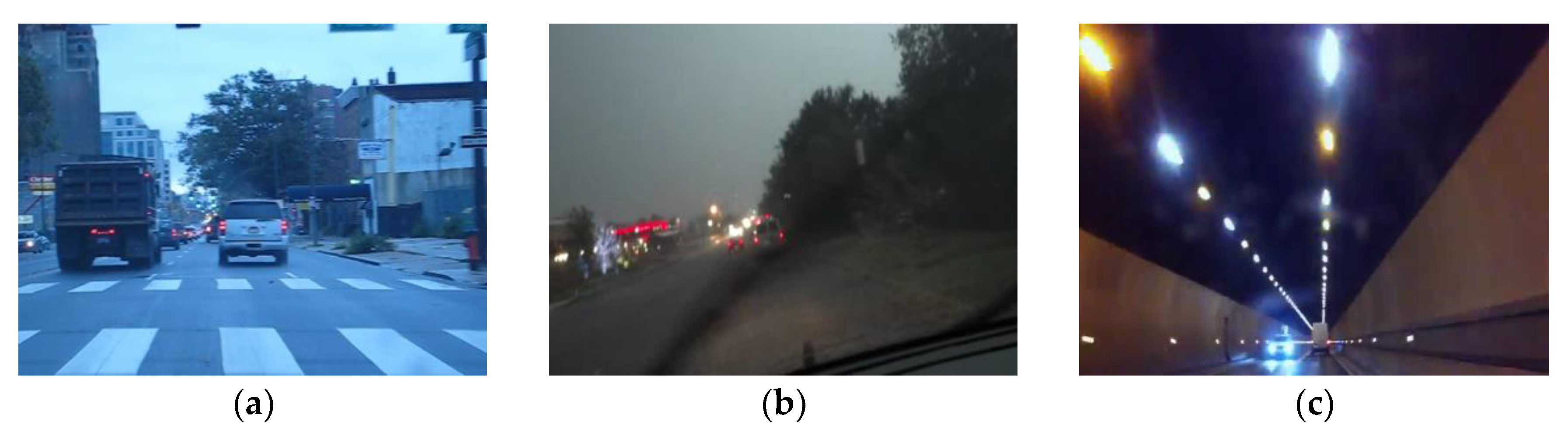
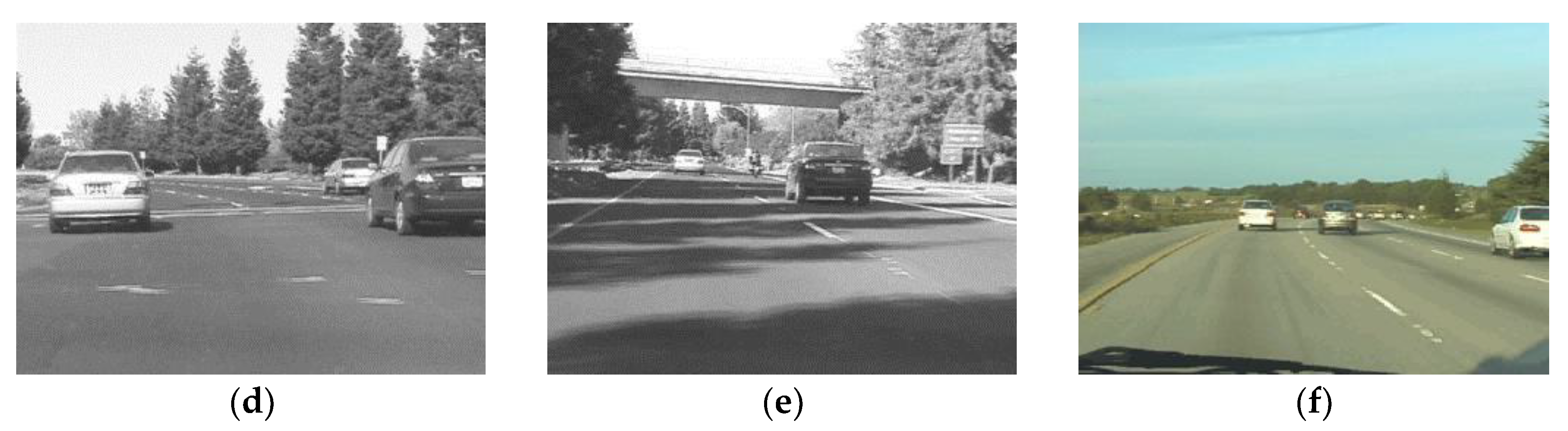
| Video | Resolution | Lighting Condition | Content Complexity |
|---|---|---|---|
| BlurCar1(2) | 640 × 480 | Medium | Medium |
| Wiper | 640 × 480 | Low | High |
| Tunnel | 640 × 360 | Low | Medium |
| Car1(1) | 320 × 240 | High | Medium |
| Car1(2) | 320 × 240 | High | Low |
| Car24 | 320 × 240 | High | Low |
© 2018 by the authors. Licensee MDPI, Basel, Switzerland. This article is an open access article distributed under the terms and conditions of the Creative Commons Attribution (CC BY) license (http://creativecommons.org/licenses/by/4.0/).
Share and Cite
Mei, Y.; Li, F.; He, L.; Wang, L. Joint Source and Channel Rate Allocation over Noisy Channels in a Vehicle Tracking Multimedia Internet of Things System. Sensors 2018, 18, 2858. https://doi.org/10.3390/s18092858
Mei Y, Li F, He L, Wang L. Joint Source and Channel Rate Allocation over Noisy Channels in a Vehicle Tracking Multimedia Internet of Things System. Sensors. 2018; 18(9):2858. https://doi.org/10.3390/s18092858
Chicago/Turabian StyleMei, Yixin, Fan Li, Lijun He, and Liejun Wang. 2018. "Joint Source and Channel Rate Allocation over Noisy Channels in a Vehicle Tracking Multimedia Internet of Things System" Sensors 18, no. 9: 2858. https://doi.org/10.3390/s18092858
APA StyleMei, Y., Li, F., He, L., & Wang, L. (2018). Joint Source and Channel Rate Allocation over Noisy Channels in a Vehicle Tracking Multimedia Internet of Things System. Sensors, 18(9), 2858. https://doi.org/10.3390/s18092858