1. Introduction
The Global Positioning System (GPS) and other global navigation satellite systems (GNSS) offer unmatched accuracy for outdoor positioning, navigation, and timing (PNT) applications. As a result, the world’s reliance on GNSS has grown significantly in the past decade. However, many applications that depend on GNSS for PNT do so without a backup should GNSS fail [
1]. For navigation applications, GNSS are inherently limited to environments with a clear view of the sky and areas that are free of large obstacles that attenuate satellite signals or cause multi-path interference. Furthermore, GNSS are susceptible to both intentional and unintentional interference which can prevent reliable navigation with these systems within affected areas. The inability to navigate in areas where GNSS are either unreliable or unavailable can have severe consequences for many users [
2]. Therefore, it is of significant interest to develop technologies that provide reliable navigation where GNSS performance is denied or degraded.
Advancements in micro-electro-mechanical systems (MEMS) technology have given rise to the smartphone as a suitable platform for pedestrian navigation. Smartphones are equipped with GNSS receivers which provide primary positioning information, as well as an array of MEMS sensors that can be used to improve positioning solutions with sensor fusion techniques. Much research has been conducted on the use of smartphones as navigation platforms [
3,
4,
5,
6,
7,
8,
9]. However, very few of the technologies proposed in the literature offer navigation solutions that can operate without the aid of external signals, such as GPS or WiFi, or additional hardware, such as high-quality inertial measurement units, antennas, and receivers.
This research expands upon the work completed by Smagowski, Raquet, and Kauffman [
10], which demonstrated the feasibility of a non-GNSS pedestrian navigation algorithm that uses only the existing sensors on a smartphone and a digital elevation model (DEM) (i.e., an elevation map). The accuracy achieved by the algorithm was promising; however, the results were obtained by post-processing smartphone data on a desktop computer. Additionally, the algorithm was evaluated using a single DEM source with very fine resolution (2 m post spacing) and a high degree of accuracy (0.3 m root mean square error (RMSE)). To take the proof-of-concept further, this research endeavored to meet the following objectives:
Implement the Smagowski et al. algorithm in a real-time smartphone application
Characterize the effect of DEM resolution and accuracy on the algorithm’s performance
Incorporate design features that increase the robustness of the algorithm
The system developed for this research was deployed on chest-mounted Android smartphones and tested at several locations using a variety of DEM sources. The results from testing showed the system is capable of achieving reliable positioning with errors that do not grow as a function of time. The accuracy of the system is terrain-dependent, but typically stays within tens of meters. For a non-GNSS outdoor pedestrian navigation system, this level of accuracy is adequate for many applications. The system could also be adopted as the base algorithm for other non-GNSS technologies, such as signals of opportunity or magnetic anomaly map-matching approaches, to further enhance position accuracy and reliability in GNSS-denied environments.
2. Materials and Methods
The centerpiece of the algorithm used in this research is the particle filter, which is a sequential Monte Carlo method commonly used to solve Bayesian estimation problems for systems with non-linear, non-Gaussian dynamics or measurements [
11]. The goal of Bayesian estimation is to recursively estimate the posterior probability density function (PDF) of hidden states in a modeled system based on observations and system inputs. For a non-linear, non-Gaussian system, this PDF is often analytically intractable, which limits the usefulness of many traditional filtering approaches. The particle filter approximates the posterior PDF of the states using a set of weighted samples or particles obtained from a different PDF that is relatively easy to draw from and has the same support as the true density [
12]. As the number of particles used in the approximation increases, the estimated PDF approaches the true PDF, and the filter solution approaches the optimal Bayesian estimate in the minimum mean square error (MMSE) sense [
13,
14]. Specifically, we used the Sequential Importance Resampling (SIR) particle filter variant described in [
11].
2.1. Algorithm Overview
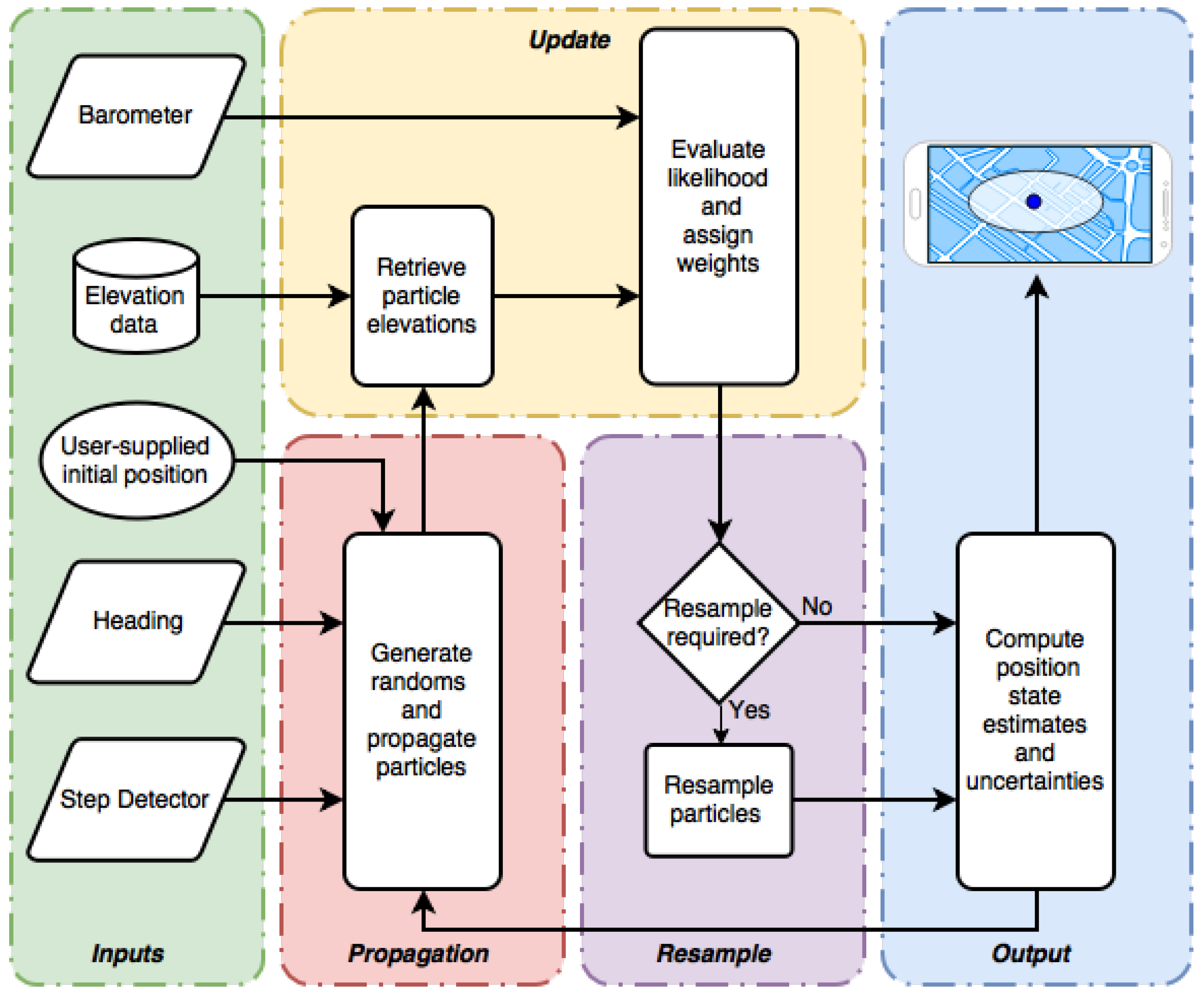
Figure 1 shows a functional block diagram of the particle filter algorithm used in this research, which was adapted from [
10]. The algorithm begins in the input stage (green) with the user providing the starting location, which is assumed to be accurate to within 5 m. This position information is used to initialize the particle filter. Once initialized, the system remains idle until a step is detected (see
Section 2.5.1), at which point the particles are propagated using the current heading input and randomly generated values for step length deviations and biases (see Equation (
4)). The particle weights remain unchanged during propagation.
When a barometric elevation measurement is available, the elevation corresponding to each particle’s location is extracted from the DEM in the update stage (yellow). A likelihood function (Equation (
7)) is then evaluated which assigns particle weights based on how closely each particle’s elevation matches the realized measurement. Particles with elevations that closely match the barometric elevation are highly weighted and are therefore more influential in the final position solution, whereas low-weighted particles are less likely and contribute very little to the solution.
After the update stage, a resampling scheme is executed, if needed, which replaces particles with negligible weights with highly weighted particles (see
Section 2.4.1). This effectively kills off particles that are likely carrying incorrect state estimates, and adds more particles to areas within the state space which are more likely to be correct. Lastly, the position estimate and associated uncertainty is computed from the weighted particles (see Equations (
8) and (
9)) and displayed on the smartphone’s display as a location marker and error ellipse in the output stage (blue). The particles used for this computation are either continually updated as new barometer measurements become available or are propagated again once the next step is detected.
2.2. Stochastic Model and Particle Filter Formulation
In this section, a state space representation of the navigation system is presented which mathematically models pedestrian motion, system inputs, barometer sensor measurements, and random noise. This stochastic model serves as the foundation for the particle filter and provides insight into the parameters that affect filter performance. The generic parameters introduced in this section are fully defined in
Section 2.5 which covers filter tuning and sensor data conditioning.
The states of interest for the system include two position states and two bias states. The two position states,
x and
y, represent the distances from the starting location (provided by the user) in the east and north directions, respectively. The heading bias state,
, represents the time-varying error in the system’s heading input, and is modeled as a first-order Gauss–Markov (FOGM) process [
15]. The barometric elevation bias state,
, represents the time-varying error in the barometric elevation measurement, and is also modeled as a FOGM process. The state vector for the system is
The individual particles are composed of two attributes, namely, a state mean estimate ( is the 4 × 1 mean vector for the ith particle at the kth step) and a weight (). The mean vector and covariance matrix for the entire particle set at the kth step are denoted by and , respectively. Initially, particles are drawn from a normal distribution, with a mean () corresponding to the initial position and bias state estimates, and a covariance () corresponding to the uncertainty of those estimates. The number of particles used is denoted by N. Upon initialization, the particles are equally weighted, such that for N. Once initialized, the particle filter’s state mean and covariance estimates are formed recursively in two stages: propagation and measurement update.
2.3. State Propagation
With each step taken, the state mean vector is propagated by a non-linear state transition function of the prior state mean vector, heading (
), average step length (
), time passed since the last propagation (
), and process noise (
). The generic equation for propagating between consecutive steps taken is
This model assumes that any uncertainty in the
x and
y states is strictly a function of other sources of uncertainty, namely, heading and step length. The process noise vector for the model,
, is given by
where
represents random deviations in step length;
and are driving white noises for the FOGM states; and
The step length deviation (
) is modeled as a uniformly-distributed random variable, as was the case in the Smagowski et al. algorithm [
10]. This assumption was made in order to bound the total step length and avoid unrealistic deviations, as would be the case in the tails of a normal distribution. The standard deviations (
) and time constants (
) are tunable FOGM parameters that control the magnitude and frequency content of the modeled biases [
15]. The process noise is assumed to be independent.
When a step is detected, the particles are propagated independently using the following equation:
In Equation (
4), the first two rows propagate the position states via pedestrian dead reckoning (PDR), which computes a new position from the previous position given the current step length and heading inputs [
4]. In this case, the system inputs are the average step length plus a random deviation and the current heading reported by the smartphone sensors (see
Section 2.5.2) plus the heading bias estimate from the prior step. The last two rows in Equation (
4) propagate the bias states according to the standard FOGM dynamics, as defined in [
15]. Note that, while the process noises associated with the FOGM biases are additive with respect to the states, the noise in the step length is multiplicative.
2.4. Measurement Update
The measurement model for the system captures how the states at a given step epoch are related to the barometric elevation measurements, denoted by
z, observed at that same epoch. For an individual particle, this relationship is represented by a non-linear function that maps a particle’s position to its corresponding elevation, taking the particle’s barometric elevation bias estimate into account:
where
is the barometric elevation measurement at step k
is the additive white Gaussian measurement noise;
(,) is a function that returns the elevation at the location (,)
In practice, the true elevation returned from
(
,
) is not directly available but is instead inferred from an interpolated DEM. This interpolated elevation is prone to error due to inaccuracies in the underlying data and interpolation error (the latter being especially true for DEMs with coarse resolution). Since the DEM is not a perfect representation of the true elevation, another term should exist in Equation (
6) which models DEM error. These errors were not explicitly modeled in our implementation because doing so would significantly increase the number of particles required. Additionally, the barometric elevation bias state and measurement noise terms were able to account for these errors adequately in most cases.
With each barometric elevation measurement, the particle weights were recursively updated by determining the likelihood of the measurement given the particle’s current state estimate. The likelihood was calculated from a Gaussian PDF centered at
with covariance R, evaluated at the measurement
. The particle weights from the prior step were then multiplied by the output of the likelihood function, resulting in the updated particle weights. For an individual particle, the update equation was
This method rewards particles whose DEM elevations closely match the measured barometric elevation and penalizes particles whose position estimates are less likely to be based on the barometric elevation measurement.
Lastly, the particle filter’s state estimate and covariance were reconstructed from the particles by computing the weighted sample mean,
, and the sample covariance,
, as follows:
The position states from this computation were then presented to the user on the system’s map display, accompanied by an ellipse representation of , which corresponds to the estimate uncertainty.
2.4.1. Resampling
One problem common to particle filtering is the condition known as particle degeneracy, in which only a few particles carry non-negligible weights. Since these low-weighted particles carry no useful information, the computational resources spent on these particles are essentially wasted. The SIR particle filter addresses this issue by occasionally resampling the particles, such that low-weighted particles are replaced with highly-weighted particles. The system developed for this research uses the multinomial resampling scheme presented in [
16]. After each measurement update, the approximate number of effective particles, N
, was calculated using:
Resampling is triggered only when drops below a threshold of 0.5, indicating only 50% of the particles carry useful information.
2.5. Data Conditioning and Filter Tuning
2.5.1. Step Detection and Step Length Estimation
Step detection was implemented using Android’s stock
step detector sensor. This sensor triggers a time-stamped event when a step is detected from walking, running, or walking up stairs. The sensor has a latency of less than 2 s, making it well-suited for applications that track the number of steps in real-time, such as PDR systems [
17].
The average step length,
, was computed using the following method found in [
7]:
where
is a gender specific constant (0.415 for males, 0.413 for females) and
is the height of the user in meters. In the propagation stage, this average step length is summed with a random step length deviation drawn from a uniform distribution,
, to account for uneven step lengths. The bounds associated with
were tuned to
= 0.15 m (6 in).
2.5.2. Heading Input and Heading Bias
The system’s heading input was implemented using Android’s
rotation vector sensor, which fuses the MEMS accelerometer, gyroscope, and magnetometer outputs to estimate the smartphone’s orientation in the world frame [
17,
18]. The output from the
rotation vector sensor was converted into a true north-referenced heading by adding the appropriate declination angle from a look-up table. The true north-referenced heading was used as the heading input,
, in Equation (
4).
The heading bias state FOGM parameters were tuned using observations from a wide range of datasets collected for this research. The reference heading bias was derived by subtracting from the heading based on the GPS data. In most cases, the reference heading biases observed were frequently changing and were bounded by . Therefore, the heading bias state was tuned such that = and = 60 s.
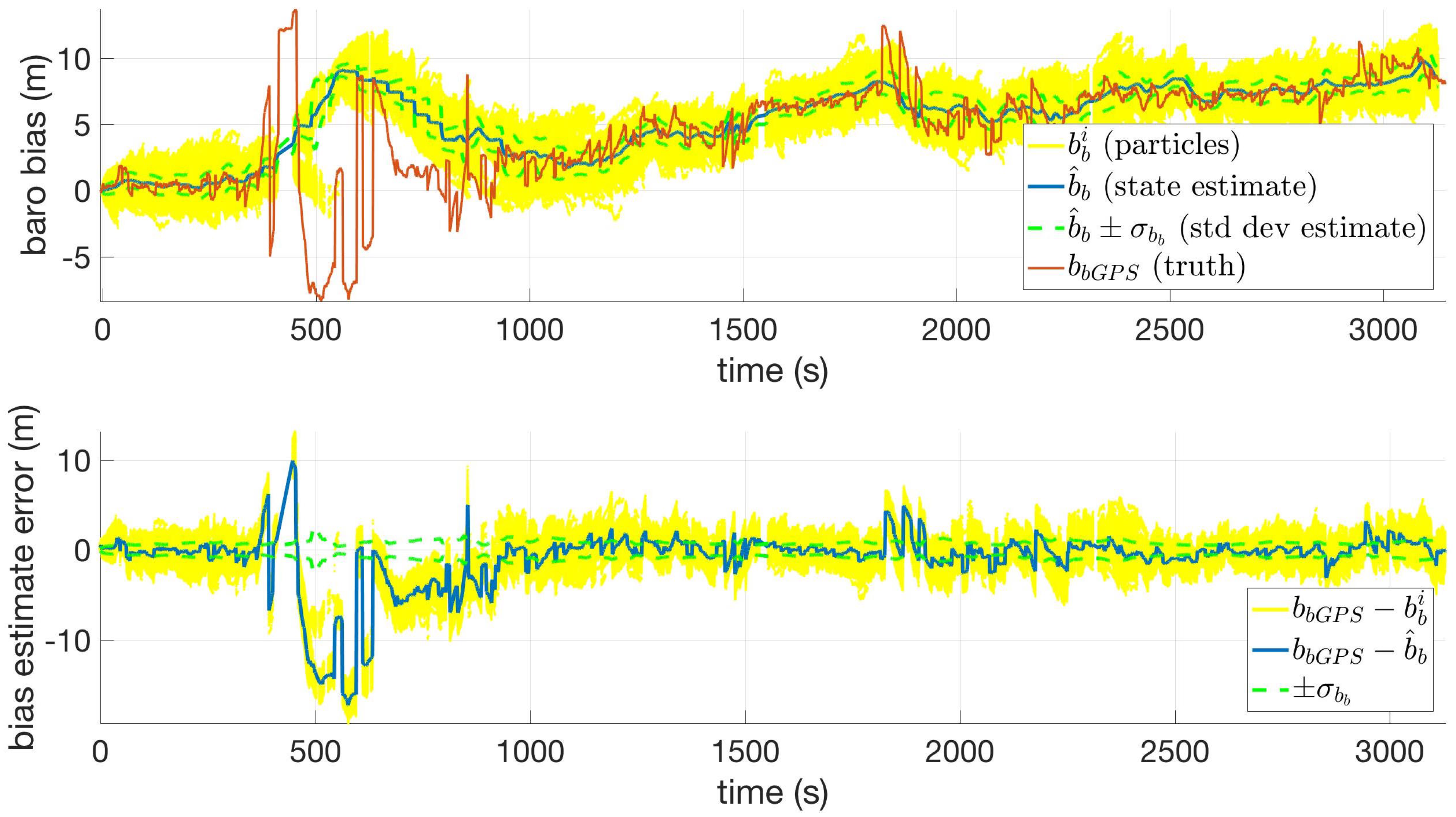
2.5.3. Barometric Elevation Bias and Measurement Noise
The barometric pressure sensors equipped in the smartphones used in this study are fairly sensitive with a data resolution of 0.16 Pa which equates to less than 10 cm of altitude [
19]. In order to tune the FOGM parameters associated with the barometric elevation bias state, barometric elevation measurements from the collected data were compared with the corresponding DEM elevations at the GPS positions reported during the collection. The difference between these values served as the reference bias, and the tuning parameters were chosen based on this reference. For the majority of DEM sources used, tuning the barometric elevation bias such that
= 5 m and
= 3600 s resulted in an adequate representation of the reference bias. For the Shuttle Radar Topography Mission (SRTM) DEM, an alternate tuning of
= 20 m and
= 1200 s was used to account for the inaccuracies present in the DEM and to avoid filter divergence issues (the accuracy and resolution specifications of the DEMs used in this research are covered in
Section 2.6.3).
The measurement noise variance, R, works in concert with the barometric elevation bias state to account for barometer sensor noise; however this parameter also accounts for errors in the underlying elevation data. Intuitively, R can be thought of as the level of confidence in how well the realized measurements will match the elevation data. Through trial and error, this value was tuned to R = 16 , which yielded reasonable performances for DEMs with 0.5, 2, and 10 m resolutions. For DEMs with 30 m resolution, an alternate tuning of R = 160 was needed to achieve a reliable performance.
2.6. Experiment Set Up
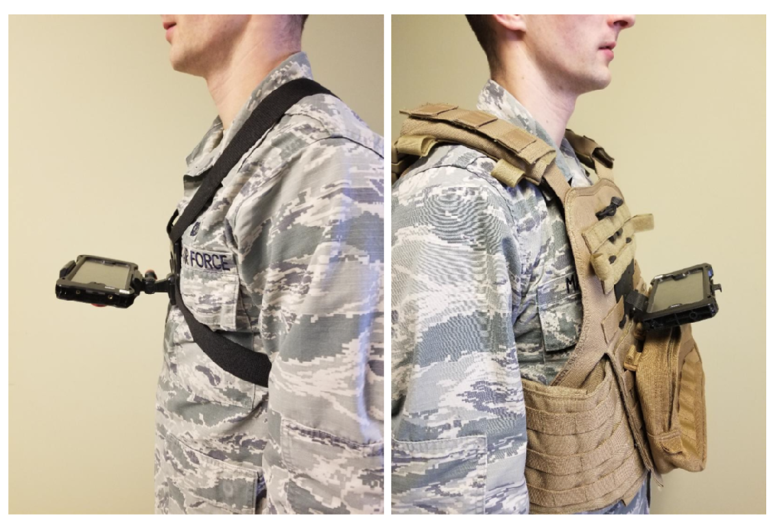
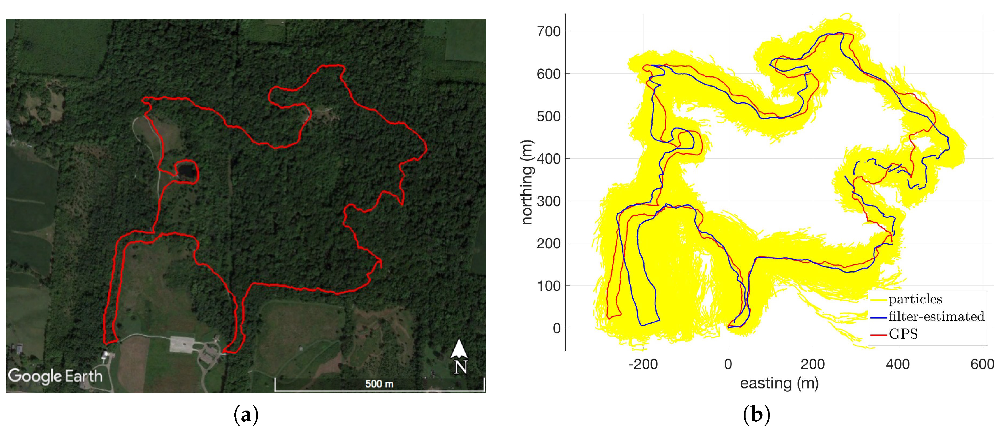
2.6.1. Data Collection
Data collection consisted of walking routes with chest-mounted smartphones running the application developed for this research. The chest mounts used are shown in
Figure 2. The smartphone models tested include the Samsung Galaxy S7, Motorola Nexus 6, and LG Nexus 5X. In addition to monitoring the real-time display during the experiments, the sensor data was recorded and replayed through an Android Studio-emulated smartphone configured with the same software but loaded with a different DEM. This was repeated for each DEM source acquired for this research, allowing for a comparison of the algorithm’s performance for a given route with respect to DEM accuracy and resolution.
While the emulator itself is a simulation, the results obtained via emulator were considered equivalent to real data for the following reasons. First, the code executed in the emulator was identical to that in the smartphone and was operating on the same sensor data obtained from the real-world experiments. Second, for a specific route/DEM combination, there was no discernible performance difference in the results obtained via emulator versus those obtained from a smartphone. Lastly, the number of particles used in the emulator was intentionally restricted to reflect the processing limitations of smartphones. The smartphone models tested for this research were able to handle up to 500 particles without any significant lag in the results. Therefore, all emulator-generated results supporting conclusions about the performance of the system were conducted with only 500 particles. This number only reflects the limitation of the system in its current implementation, since there are many ways to optimize the software that would allow for more particles to be carried.
2.6.2. Performance Metrics
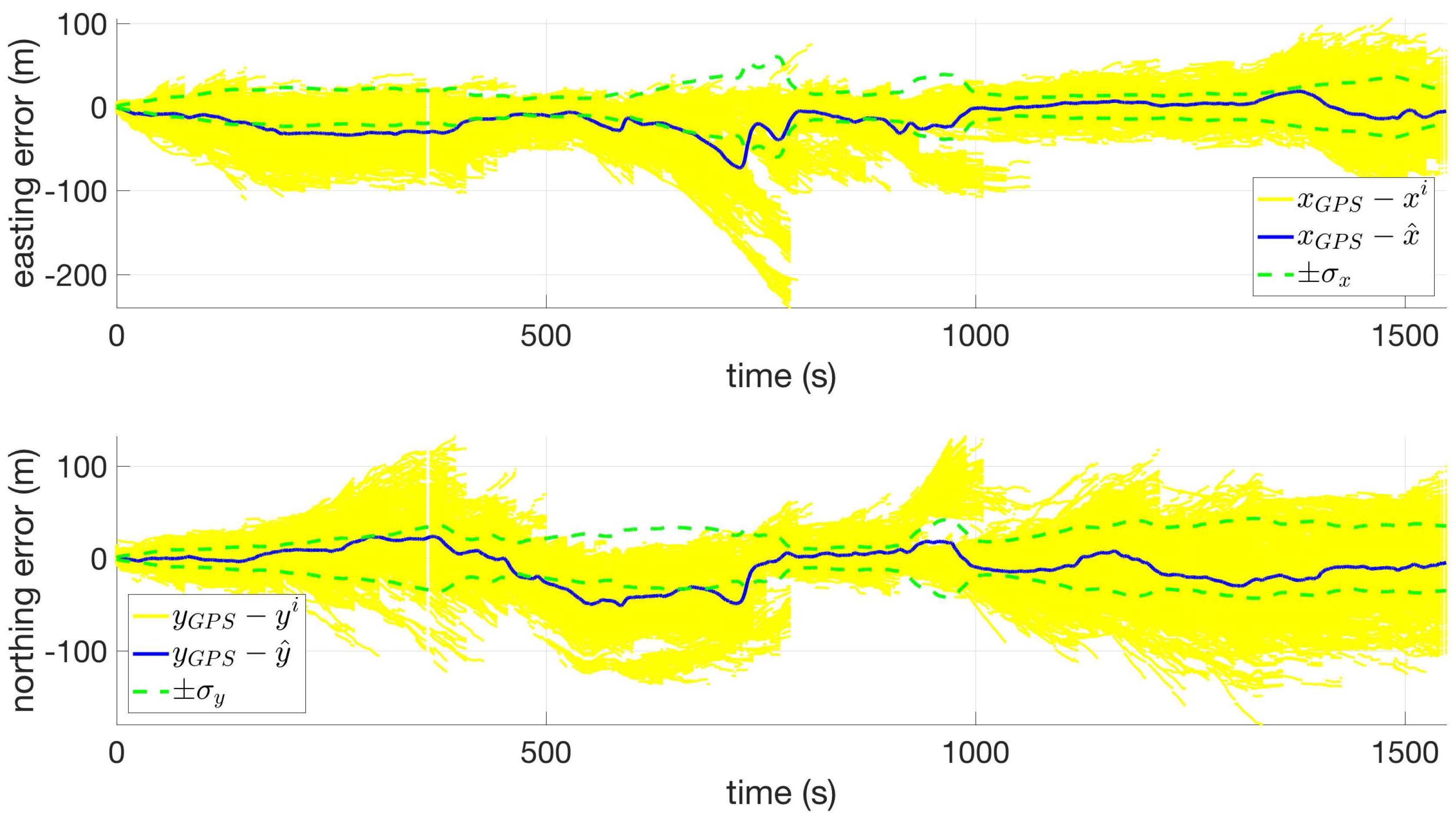
The performance of the system was quantified by the distance root mean square (DRMS) error with respect to GPS (recorded for comparison only, not used in the algorithm), given by
In Equation (
12),
n is the number of steps taken during the route, and
is the Euclidean horizontal distance measured from the interpolated GPS position to the filter-estimated position at the
kth step. In two cases, the smartphones were configured with airplane mode turned on and location services turned off for all or some of the route. This was to simulate a GNSS-denied environment. As a result, the DRMS values reported for those trials were only calculated at step epochs during which GPS was turned on.
2.6.3. Elevation Data Sources
The five DEMs acquired for this research are listed in
Table 1. The tags in the second column are used to differentiate results obtained using these DEMs throughout this article. All of the sources listed are freely available online, with the exception of the VDTM0.5 which was donated courtesy of Vricon. The availability of the DEMs are also listed in
Table 1, which was an important consideration for this research due to the algorithm’s dependency on elevation data. While only the SRTM and Vricon are globally available, many countries have agencies that provide products and services similar to the U.S. Geological Survey (USGS). Also, the popularity of lidar has grown in recent years, and efforts are underway to create an open-source global lidar database as these products become available [
20]. The last two columns of
Table 1 list the resolution and the accuracy specifications for the DEMs. The resolutions range from very coarse (30 m post spacing) to very fine (0.5 m post spacing). The Ohio Statewide Imagery Program (OSIP) DEM is significantly more accurate than the rest of the DEMs, whereas the USGS and Vricon DEMs have similar accuracy specifications, and the SRTM DEM is the least accurate by a wide margin.
2.6.4. Testing Locations
In order to better understand the effects of terrain on the system’s performance, testing locations were categorized based on their respective elevation profiles. Routes consisting of less than 10 m of elevation change throughout the route were categorized as flat terrain. Routes consisting of steadily changing elevation with more than 10 m of total elevation change were categorized as slanted terrain (i.e., steep hills). Routes consisting of high spatial-frequency changes in elevation were categorized as varied terrain. There were six distinct testing locations, two of each category (flat, slanted, and varied). Experiments were conducted outdoors under a variety of weather conditions, including sub-zero air temperatures, high wind speeds, snow, and rain.
4. Discussion
The results from testing indicate the system is capable of achieving positioning accuracies in the tens of meters, with positioning errors that do not grow as a function of time. The accuracy of the system depends on the elevation diversity of the terrain and the accuracy of the elevation map, and is therefore not directly related to the distance traveled. Positioning errors less than 48 m DRMS can be achieved using DEMs with 10 m post spacing or less, provided the DEM’s accuracy is 3 m (RMSE) or less. The system’s performance was adequate (less than 61 m DRMS error) when using the USGS’s 30 m post spacing DEM. Of the DEM sources tested, Vricon, OSIP, and USGS are all viable options. Marginal accuracy improvements were observed when using NASA’s 30 m SRTM DEM for most of the datasets; however, in some cases, filter tuning issues and particle starvation resulted in unsatisfactory performances.
One aspect of performance not captured by the tables presented in this article is the filter-predicted uncertainty associated with the position estimates. As discussed in
Section 2.5, alternate filter tunings were needed for the 30 m DEMs to account for the resolution and errors in these datasets. The effect of using the more pessimistic tuning was that filter-predicted standard deviations were much larger than when using the tuning for DEMs with finer resolution. This was mostly due to the increased value of R. For the SRTM datasets, the alternate barometric elevation bias tuning also contributed to this increased uncertainty. More work is needed to investigate alternative methods for improving the performance of the system when using SRTM30, such as increasing the number of particles or using another set of tuning parameters.
The system operates in near real-time, and there was no perceptible initialization time or time lag in the results observed during operation. There were some cases in which the filter became overconfident and falsely locked onto an incorrect positioning solution. This was often caused by a variety of factors, including modeling error (i.e., step lengths that were much shorter than the model allows), weather effects (high wind speeds inducing fluctuations in the barometer), and similarities in the elevation profiles of the correct and incorrect paths. While beyond the scope of this article, a residual monitoring subroutine was implemented to detect and cope with these situations which effectively aided the filter in recovering the correct position.
The primary advantage of the system presented in this article over other non-GNSS outdoor smartphone positioning systems is that it is self-contained, that is, since the system requires no external reference signals or additional equipment, it is lightweight and immune to jamming. However, environmental interference can negatively affect the system’s performance, specifically, through the presence of man-made sources of magnetic fields, such as buildings made of steel or power transmission lines which can induce magnetometer biases that are larger than the model allows (as was the case in short-duration heading disturbance from Route 8 discussed in
Section 3.2). Although the data presented in this article was not collected in dense urban canyons, it is reasonable to assume that the system’s performance could suffer in these environments. Future work should examine the system’s performance in areas densely populated with man-made structures.
Another area of improvement for the system presented in this article is the step length model, which is admittedly simplistic and could be a significant source of positioning error. Future work should consider more sophisticated techniques, such as that used in reference [
29], which proposed an empirical model based step frequency, user height, and acceleration amplitude, or reference [
30], which proposed using GPS measurements to estimate a set of gait parameters for a specific user (for our purposes, these parameters could be learned and stored prior to using the system in a GPS-degraded environment).


