Rectification of Images Distorted by Microlens Array Errors in Plenoptic Cameras


Abstract
:1. Introduction
2. Models
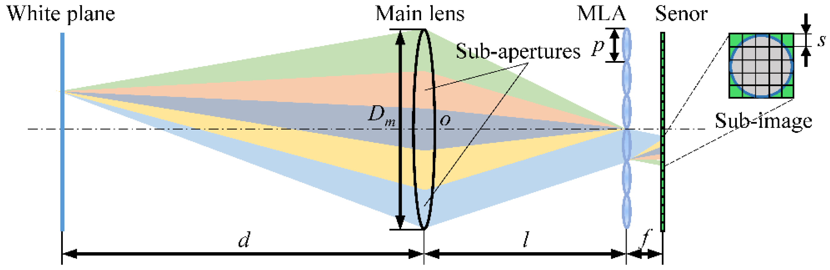
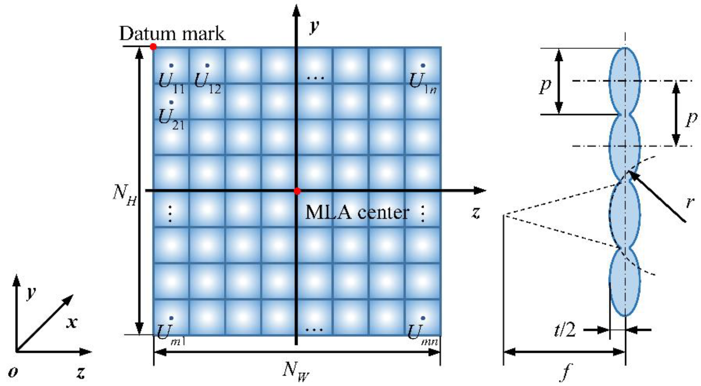
2.1. Light-Field Imaging Model
2.2. MLA Surface Error Model
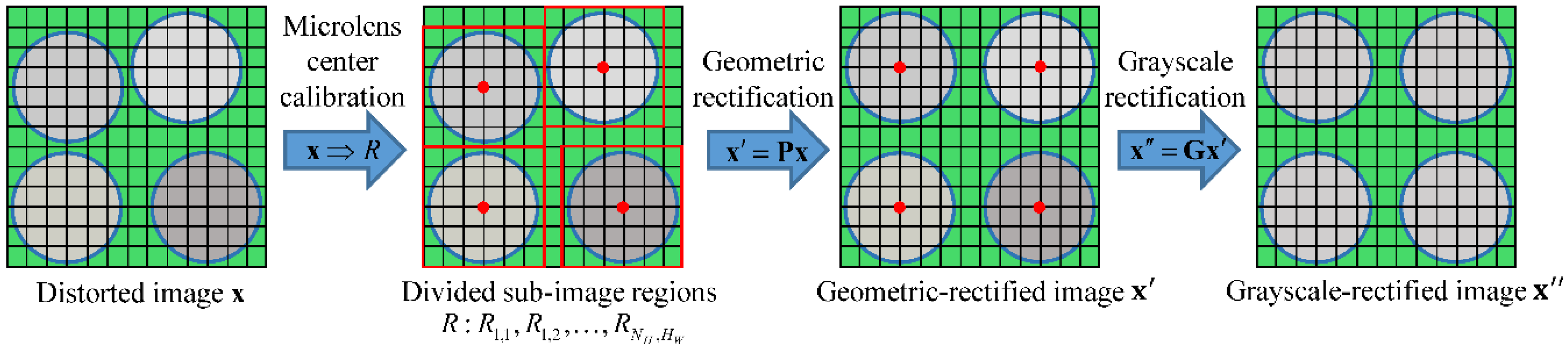
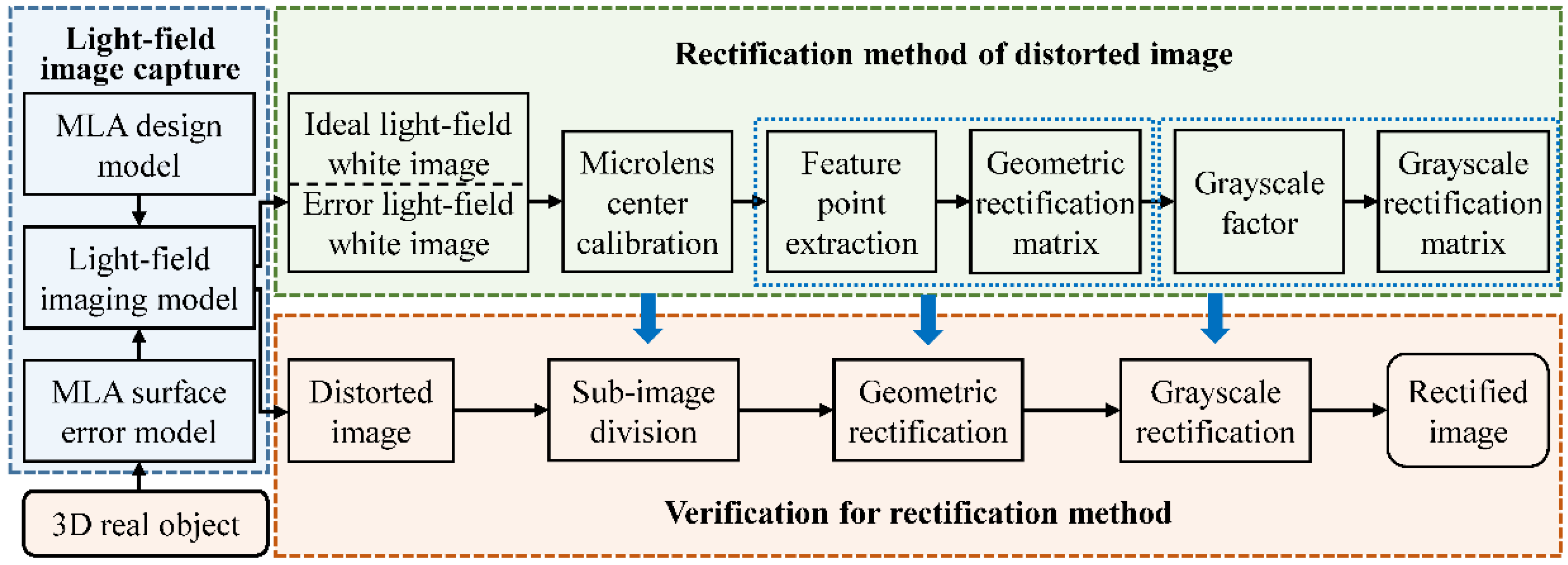
3. Rectification Method
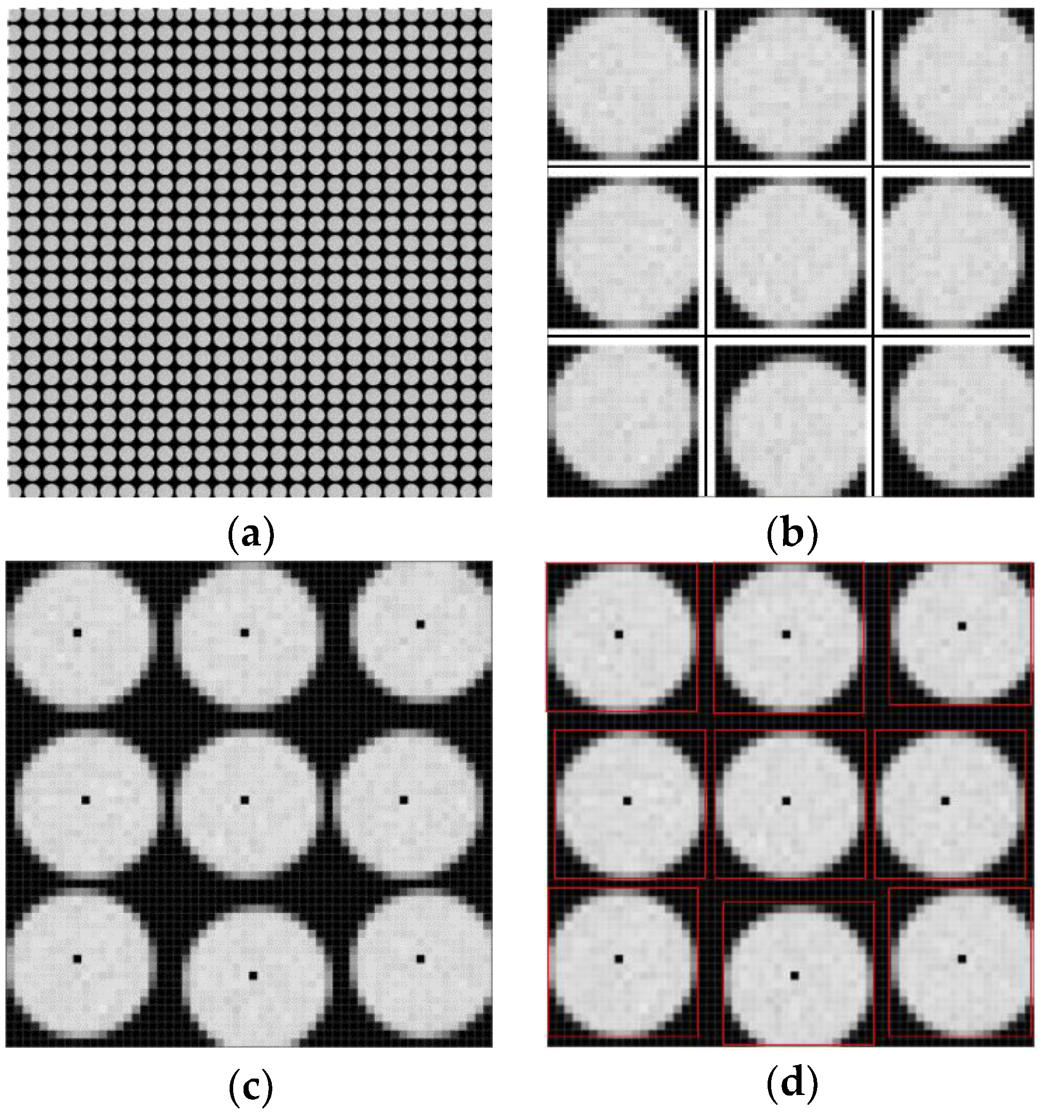
3.1. Microlens Center Calibration
3.2. Geometric Rectification
3.3. Grayscale Rectification
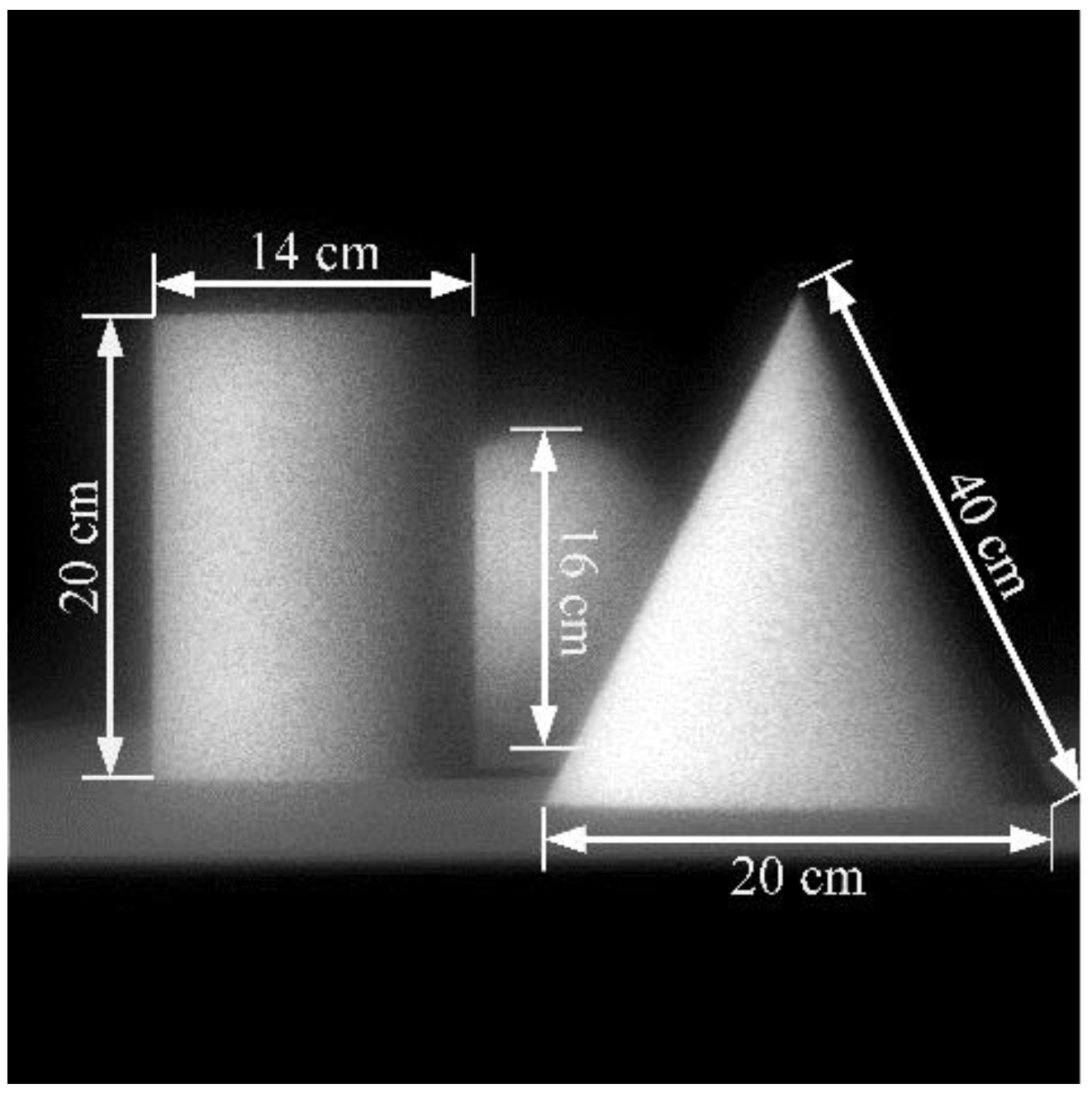
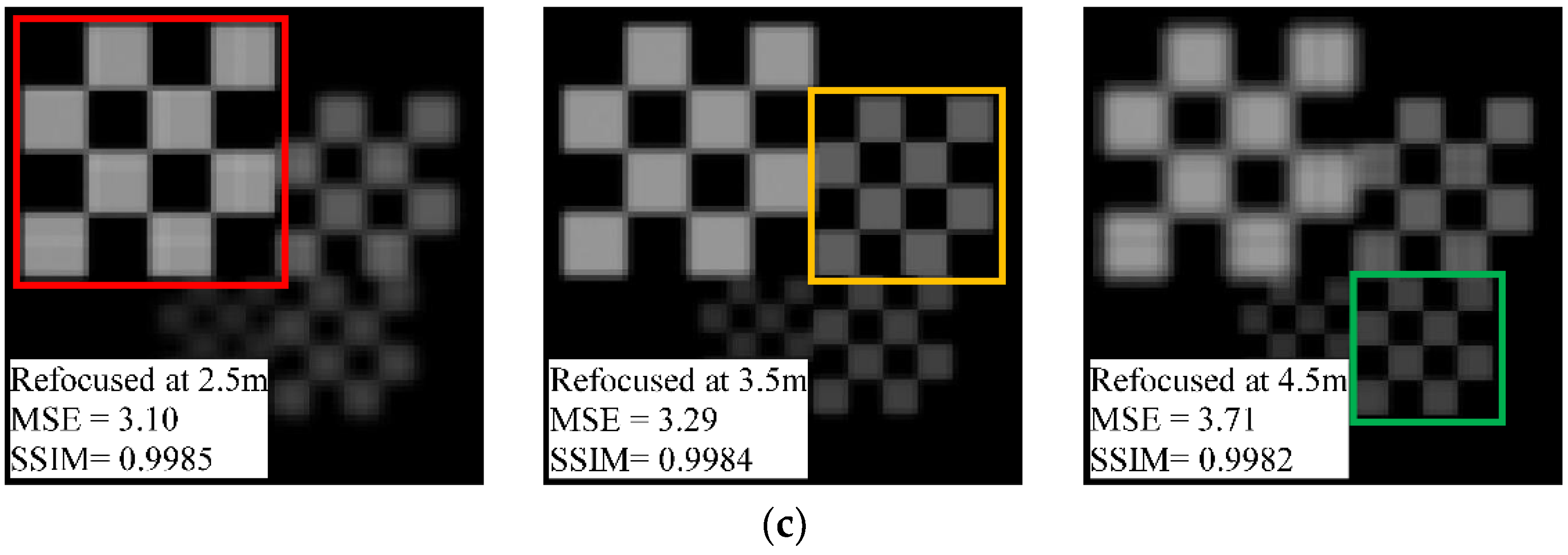
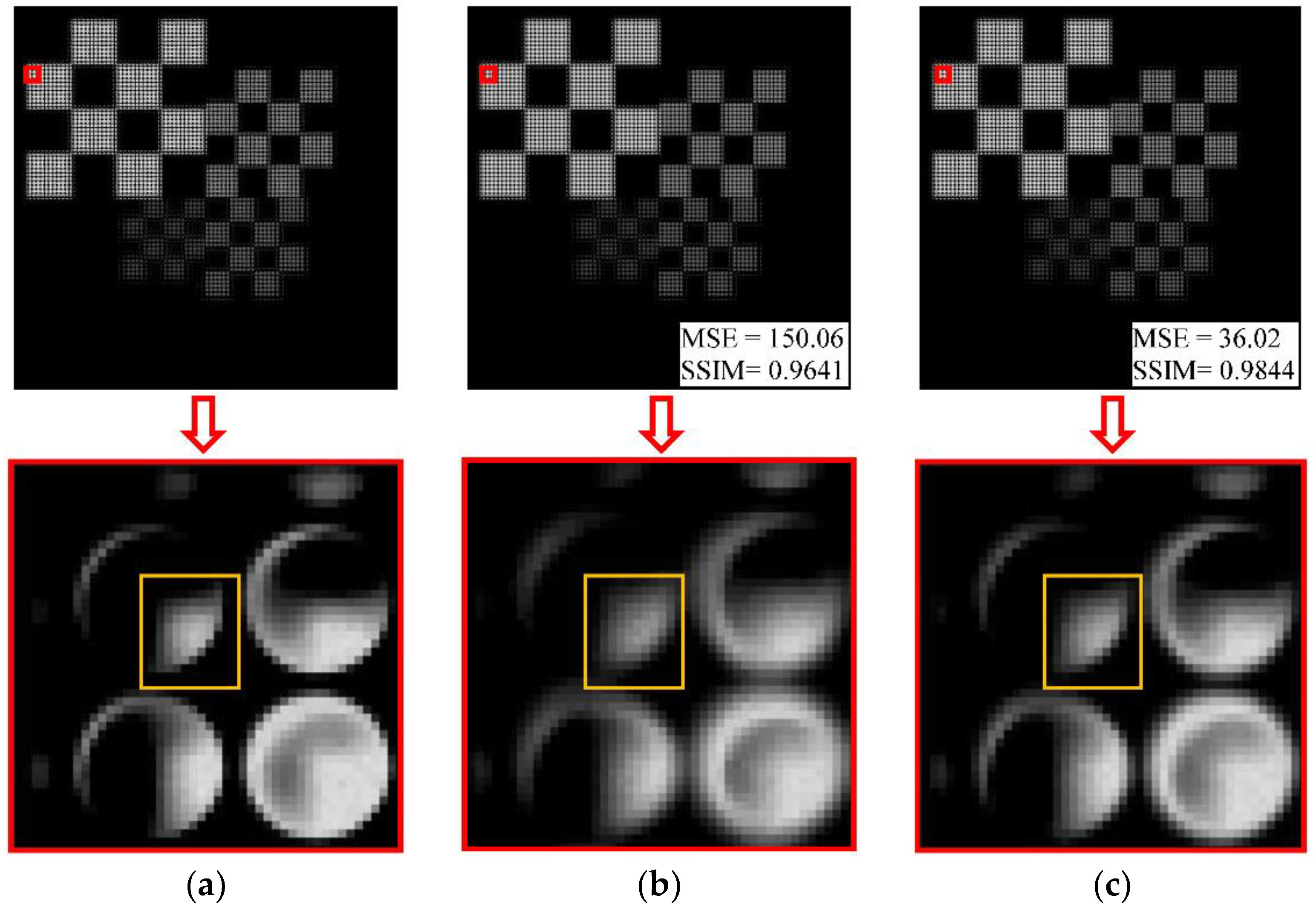
4. Results and Analysis
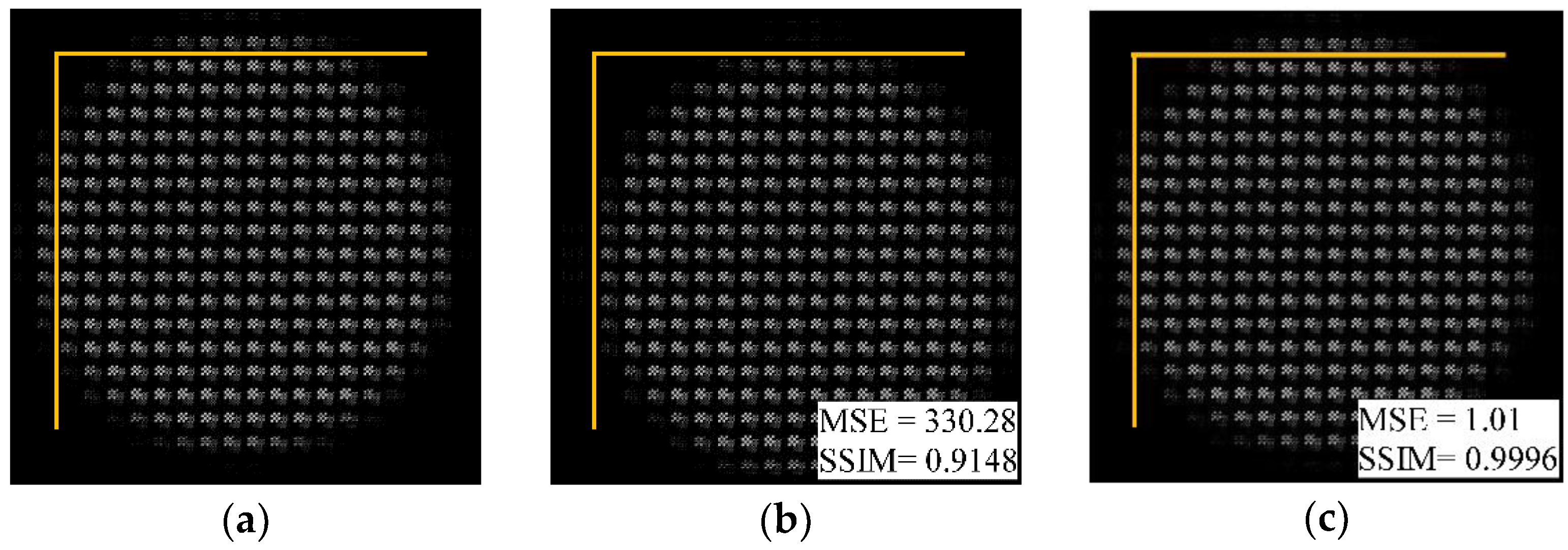
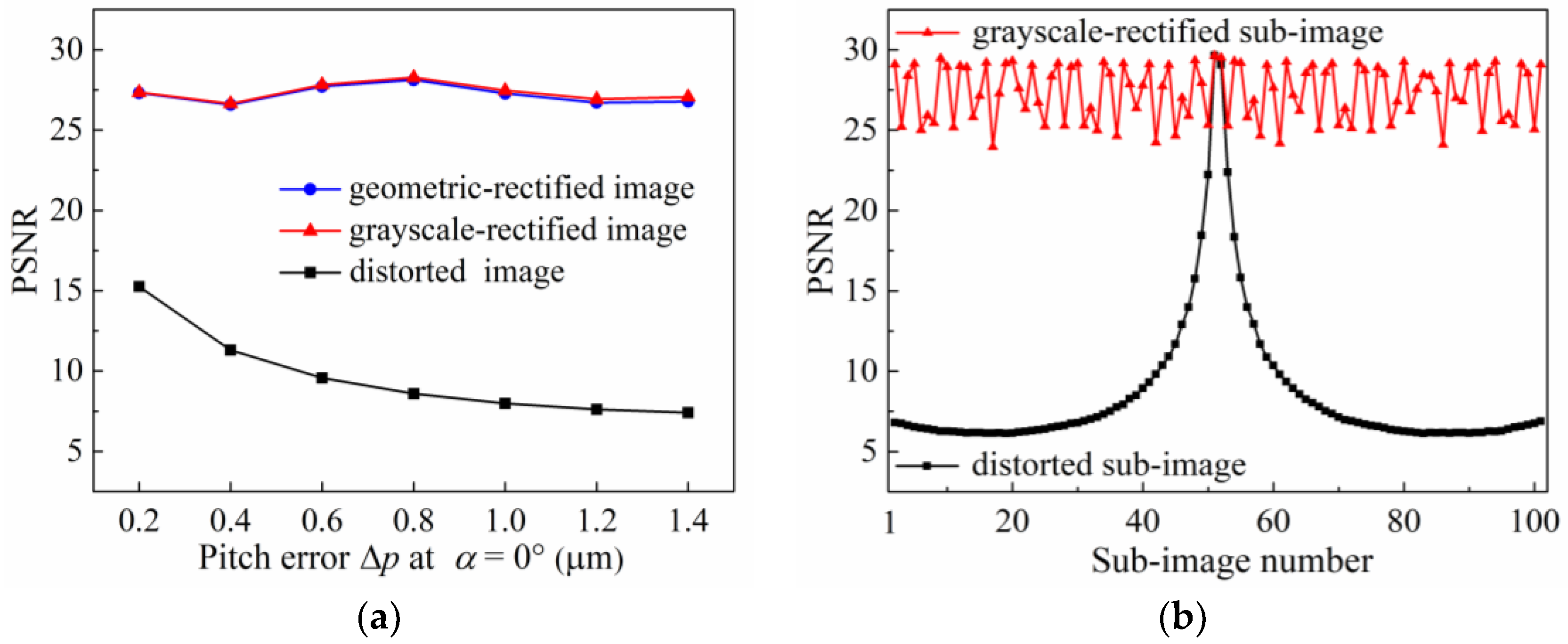
4.1. Pitch Error
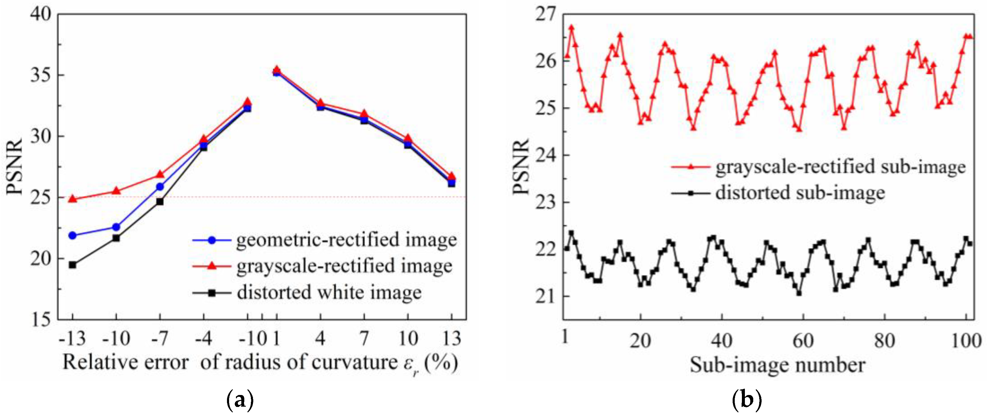
4.2. Radius-of-Curvature Error
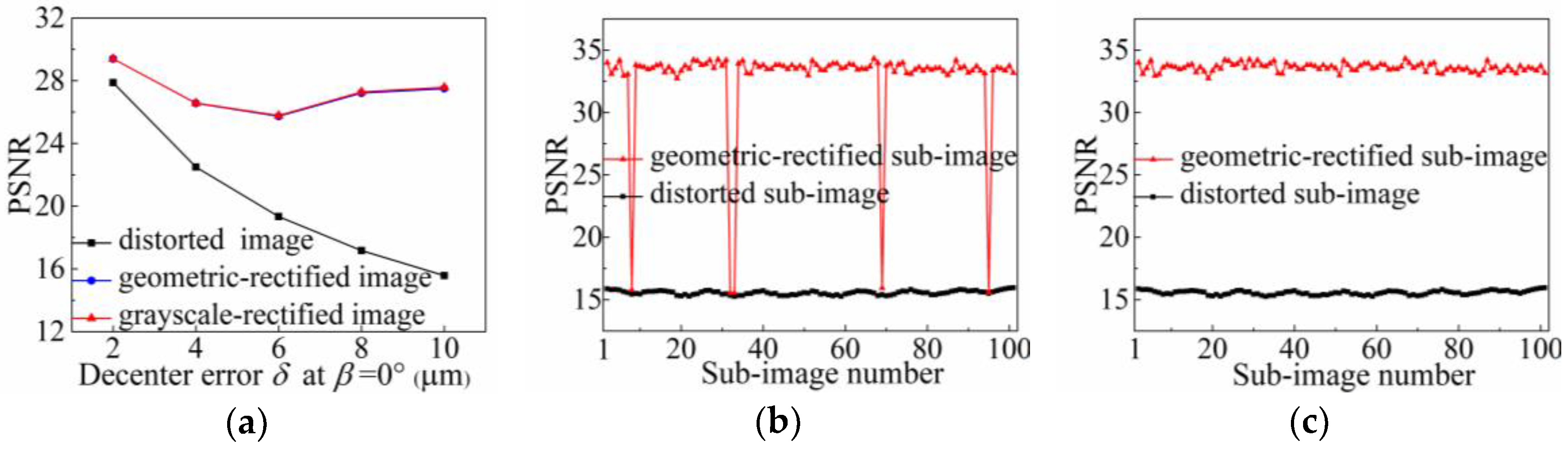
4.3. Decenter Error
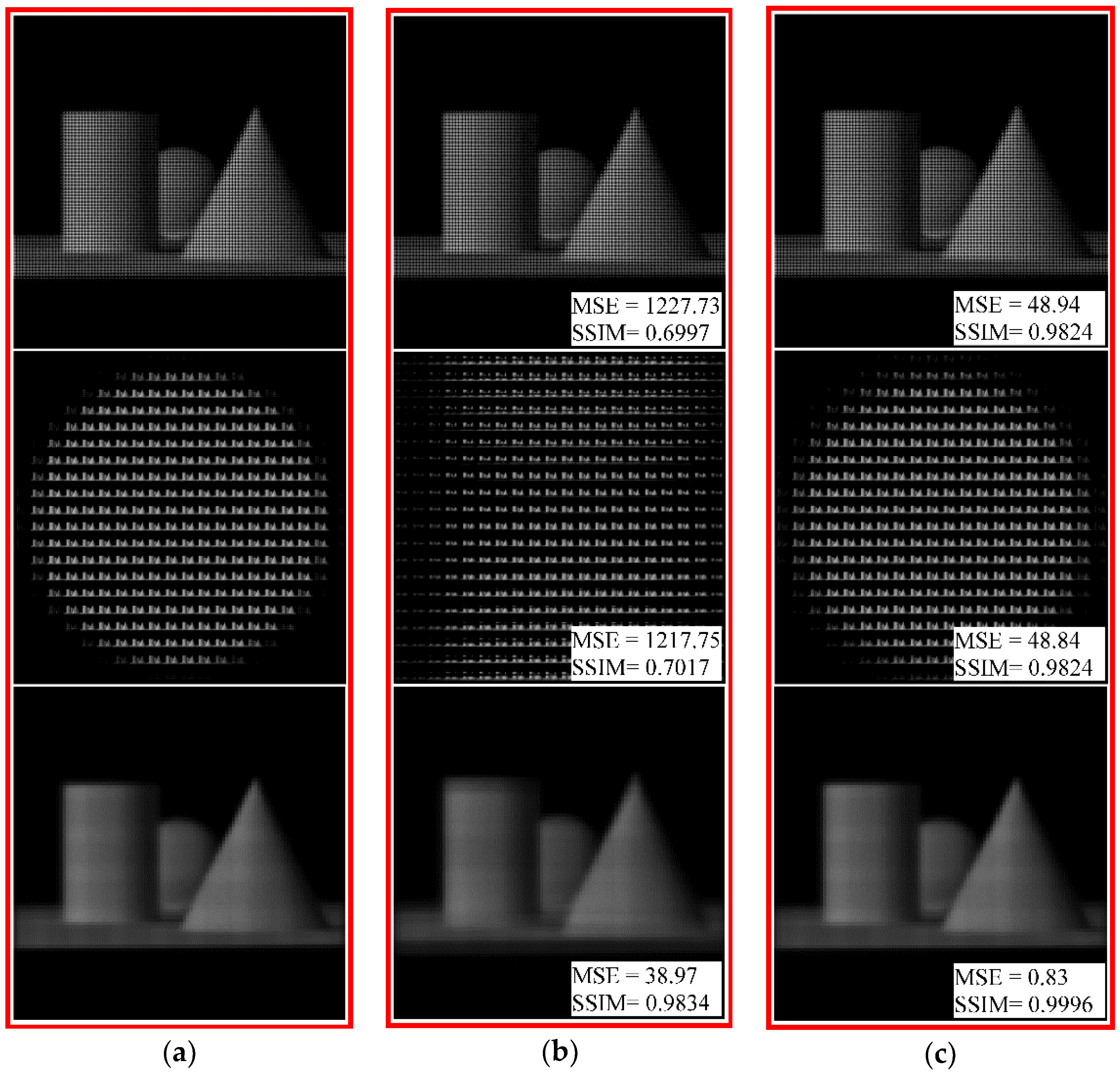
4.4. Combined Error
5. Disscussion
6. Conclusions
Author Contributions
Funding
Acknowledgments
Conflicts of Interest
References
- Levoy, M. Light fields and computational imaging. Computer 2006, 39, 46–55. [Google Scholar] [CrossRef]
- Ng, R.; Levoy, M.; Brédif, M.; Duval, G.; Horowitz, M.; Hanrahan, P. Light field photography with a hand-held plenoptic camera. Comput. Sci. Tech. Rep. 2005, 2, 1–11. [Google Scholar]
- Levoy, M.; Ng, R.; Adams, A.; Footer, M.; Horowitz, M. Light field microscopy. ACM Trans. Graph. 2006, 25, 924–934. [Google Scholar] [CrossRef]
- Georgiev, T.; Lumsdaine, A. Focused plenoptic camera and rendering. J. Electron. Imaging 2010, 19, 021106. [Google Scholar]
- Antensteiner, D.; Štolc, S.; Pock, T. A review of depth and normal fusion algorithms. Sensors 2018, 18, 431. [Google Scholar] [CrossRef] [PubMed]
- Rodríguez, M.; Magdaleno, E.; Pérez, F.; García, C. Automated software acceleration in programmable logic for an efficient NFFT algorithm implementation: A case study. Sensors 2017, 17, 694. [Google Scholar] [CrossRef] [PubMed]
- Pérez, J.; Magdaleno, E.; Pérez, F.; Rodríguez, M.; Hernández, D.; Corrales, J. Super-Resolution in plenoptic cameras using FPGAs. Sensors 2014, 14, 8669–8685. [Google Scholar] [CrossRef] [PubMed]
- Sun, J.; Xu, C.; Zhang, B.; Hossain, M.M.; Wang, S.; Qi, H.; Tan, H. Three-dimensional temperature field measurement of flame using a single light field camera. Opt. Express 2016, 24, 1118–1132. [Google Scholar] [CrossRef] [PubMed]
- Yuan, Y.; Liu, B.; Li, S.; Tan, H. Light-field-camera imaging simulation of participatory media using Monte Carlo method. Int. J. Heat Mass Transf. 2016, 102, 518–527. [Google Scholar] [CrossRef]
- Kim, S.; Ban, Y.; Lee, S. Face liveness detection using a light field camera. Sensors 2014, 14, 22471–22499. [Google Scholar] [CrossRef] [PubMed]
- Fahringer, T.W.; Lynch, K.P.; Thurow, B.S. Volumetric particle image velocimetry with a single plenoptic camera. Meas. Sci. Technol. 2015, 26, 115201. [Google Scholar] [CrossRef]
- Chen, H.; Sick, V. Three-dimensional three-component air flow visualization in a steady-state engine flow bench using a plenoptic camera. SAE Int. J. Engines 2017, 10, 625–635. [Google Scholar] [CrossRef]
- Skinner, K.A.; Johnson-Roberson, M. Towards real-time underwater 3D reconstruction with plenoptic cameras. In Proceedings of the 2016 IEEE/RSJ International Conference on in Intelligent Robots and Systems (IROS), Daejeon, Korea, 9–14 October 2016; pp. 2014–2021. [Google Scholar]
- Dong, F.; Ieng, S.H.; Savatier, X.; Etienne-Cummings, R.; Benosman, R. Plenoptic cameras in real-time robotics. Int. J. Robot. Res. 2013, 32, 206–217. [Google Scholar] [CrossRef]
- Liu, X.; Zhang, X.; Fang, F.; Zeng, Z.; Gao, H.; Hu, X. Influence of machining errors on form errors of microlens arrays in ultra-precision turning. Int. J. Mach. Tools Manuf. 2015, 96, 80–93. [Google Scholar] [CrossRef]
- Cao, A.; Pang, H.; Wang, J.; Zhang, M.; Chen, J.; Shi, L.; Deng, Q.; Hu, S. The Effects of Profile Errors of Microlens Surfaces on Laser Beam Homogenization. Micromachines 2017, 8, 50. [Google Scholar] [CrossRef]
- Thomason, C.M.; Fahringer, T.F.; Thurow, B.S. Calibration of a microlens array for a plenoptic camera. In Proceedings of the 52nd AIAA Aerospace Sciences Meeting, National Harbor, MD, USA, 13–17 January 2014; p. 0396. [Google Scholar]
- Li, S.; Yuan, Y.; Zhang, H.; Liu, B.; Tan, H. Microlens assembly error analysis for light field camera based on Monte Carlo method. Opt. Commun. 2016, 372, 22–36. [Google Scholar] [CrossRef]
- Li, S.; Yuan, Y.; Liu, B.; Wang, F.; Tan, H. Influence of microlens array manufacturing errors on light-field imaging. Opt. Commun. 2018, 410, 40–52. [Google Scholar] [CrossRef]
- Li, S.; Yuan, Y.; Liu, B.; Wang, F.; Tan, H. Local error and its identification for microlens array in plenoptic camera. Opt. Lasers Eng. 2018, 108, 41–53. [Google Scholar] [CrossRef]
- Shi, S.; Wang, J.; Ding, J.; Zhao, Z.; New, T.H. Parametric study on light field volumetric particle image velocimetry. Flow Meas. Instrum. 2016, 49, 70–88. [Google Scholar] [CrossRef]
- Fahringer, T.; Thurow, B. The effect of grid resolution on the accuracy of tomographic reconstruction using a plenoptic camera. In Proceedings of the 51st AIAA Aerospace Sciences Meeting Including the New Horizons Forum and Aerospace Exposition, Dallas, TX, USA, 7–10 January 2013; p. 0039. [Google Scholar]
- Kong, X.; Chen, Q.; Wang, J.; Gu, G.; Wang, P.; Qian, W.; Ren, K.; Miao, X. Inclinometer assembly error calibration and horizontal image correction in photoelectric measurement systems. Sensors 2018, 18, 248. [Google Scholar] [CrossRef] [PubMed]
- Lourenço, M.; Barreto, J.P.; Francisco, V. sRD-SIFT: Keypoint detection and matching in images with radial distortion. IEEE Trans Robot. 2012, 28, 752–760. [Google Scholar] [CrossRef]
- Furnari, A.; Farinella, G.M.; Bruna, A.R.; Battiato, S. Affine covariant features for fisheye distortion local modeling. IEEE Trans. Image Process. 2017, 26, 696–710. [Google Scholar] [CrossRef] [PubMed]
- Cruz-Mota, J.; Bogdanova, I.; Paquier, B.; Bierlaire, M.; Thiran, J.P. Scale invariant feature transform on the sphere: Theory and applications. Int. J. Comput. Vis. 2012, 98, 217–241. [Google Scholar] [CrossRef]
- Jin, J.; Cao, Y.; Cai, W.; Zheng, W.; Zhou, P. An effective rectification method for lenselet-based plenoptic cameras. In Proceedings of the SPIE/COS Photonics Asia on Optoelectronic Imaging and Multimedia Technology IV, Beijing, China, 12–14 October 2016; p. 100200F. [Google Scholar]
- Dansereau, D.G.; Pizarro, O.; Williams, S.B. Decoding, calibration and rectification for lenselet-based plenoptic cameras. In Proceedings of the 2013 IEEE Conference on Computer Vision and Pattern Recognition (CVPR), Portland, OR, USA, 23–28 June 2013; pp. 1027–1034. [Google Scholar]
- Cho, D.; Lee, M.; Kim, S.; Tai, Y.W. Modeling the calibration pipeline of the Lytro camera for high quality light-field image reconstruction. In Proceedings of the 2013 IEEE International Conference on Computer Vision (ICCV), Sydney, Australia, 1–8 December 2013; pp. 3280–3287. [Google Scholar]
- Li, T.; Li, S.; Li, S.; Yuan, Y.; Tan, H. Correction model for microlens array assembly error in light field camera. Opt. Express 2016, 24, 24524–24543. [Google Scholar] [CrossRef] [PubMed]
- Mukaida, M.; Yan, J. Ductile machining of single-crystal silicon for microlens arrays by ultraprecision diamond turning using a slow tool servo. Int. J. Mach. Tools Manuf. 2017, 115, 2–14. [Google Scholar] [CrossRef]
- Liu, B.; Yuan, Y.; Li, S.; Shuai, Y.; Tan, H. Simulation of light-field camera imaging based on ray splitting Monte Carlo method. Opt. Commun. 2015, 355, 15–26. [Google Scholar] [CrossRef]
- Shih, Y.M.; Kao, C.C.; Ke, K.C.; Yang, S.Y. Imprinting of double-sided microstructures with rapid induction heating and gas-assisted pressuring. J. Micromech. Microeng. 2017, 27, 095012. [Google Scholar] [CrossRef]
- Zhao, Z.; Hui, M.; Liu, M.; Dong, L.; Liu, X.; Zhao, Y. Centroid shift analysis of microlens array detector in interference imaging system. Opt. Commun. 2015, 354, 132–139. [Google Scholar] [CrossRef]
- Huang, C.Y.; Hsiao, W.T.; Huang, K.C.; Chang, K.S.; Chou, H.Y.; Chou, C.P. Fabrication of a double-sided micro-lens array by a glass molding technique. J. Micromech. Microeng. 2011, 21, 085020. [Google Scholar] [CrossRef]
- Xie, D.; Chang, X.; Shu, X.; Wang, Y.; Ding, H.; Liu, Y. Rapid fabrication of thermoplastic polymer refractive microlens array using contactless hot embossing technology. Opt. Express 2015, 23, 5154–5166. [Google Scholar] [CrossRef] [PubMed]
- Furnari, A.; Farinella, G.M.; Bruna, A.R.; Battiato, S. Generalized Sobel filters for gradient estimation of distorted images. In Proceedings of the 2015 IEEE Conference on Image Processing (ICIP), Quebec City, QC, Canada, 27–30 September 2015; pp. 3250–3254. [Google Scholar]
- Furnari, A.; Farinella, G.M.; Bruna, A.R.; Battiato, S. Distortion adaptive Sobel filters for the gradient estimation of wide angle images. J. Vis. Commun. Image Represent. 2017, 46, 165–175. [Google Scholar] [CrossRef]
- Wang, Z.; Bovik, A.C.; Sheikh, H.R.; Simoncelli, E.P. Image quality assessment: From error visibility to structural similarity. IEEE Trans. Image Process. 2004, 13, 600–612. [Google Scholar] [CrossRef] [PubMed]


| Parameters | Value |
|---|---|
| Number of microlenses NW × NH | 102 × 102 |
| Pitch (Side length) p | 100 μm |
| Radius of curvature r | 469 μm |
| Thickness at the vertex t | 10 μm |
| Focal length f | 420 μm |
| Refractive index n (λ = 632.8 nm) | 1.56 |
| Errors | Surface Description Equations |
|---|---|
| Pitch error Δp | |
| Radius-of-curva-ture error Δr | |
| Decenter error δ |
© 2018 by the authors. Licensee MDPI, Basel, Switzerland. This article is an open access article distributed under the terms and conditions of the Creative Commons Attribution (CC BY) license (http://creativecommons.org/licenses/by/4.0/).
Share and Cite
Li, S.; Zhu, Y.; Zhang, C.; Yuan, Y.; Tan, H. Rectification of Images Distorted by Microlens Array Errors in Plenoptic Cameras. Sensors 2018, 18, 2019. https://doi.org/10.3390/s18072019
Li S, Zhu Y, Zhang C, Yuan Y, Tan H. Rectification of Images Distorted by Microlens Array Errors in Plenoptic Cameras. Sensors. 2018; 18(7):2019. https://doi.org/10.3390/s18072019
Chicago/Turabian StyleLi, Suning, Yanlong Zhu, Chuanxin Zhang, Yuan Yuan, and Heping Tan. 2018. "Rectification of Images Distorted by Microlens Array Errors in Plenoptic Cameras" Sensors 18, no. 7: 2019. https://doi.org/10.3390/s18072019
APA StyleLi, S., Zhu, Y., Zhang, C., Yuan, Y., & Tan, H. (2018). Rectification of Images Distorted by Microlens Array Errors in Plenoptic Cameras. Sensors, 18(7), 2019. https://doi.org/10.3390/s18072019