Non-Contact Smartphone-Based Monitoring of Thermally Stressed Structures

 , , and
Abstract
1. Introduction
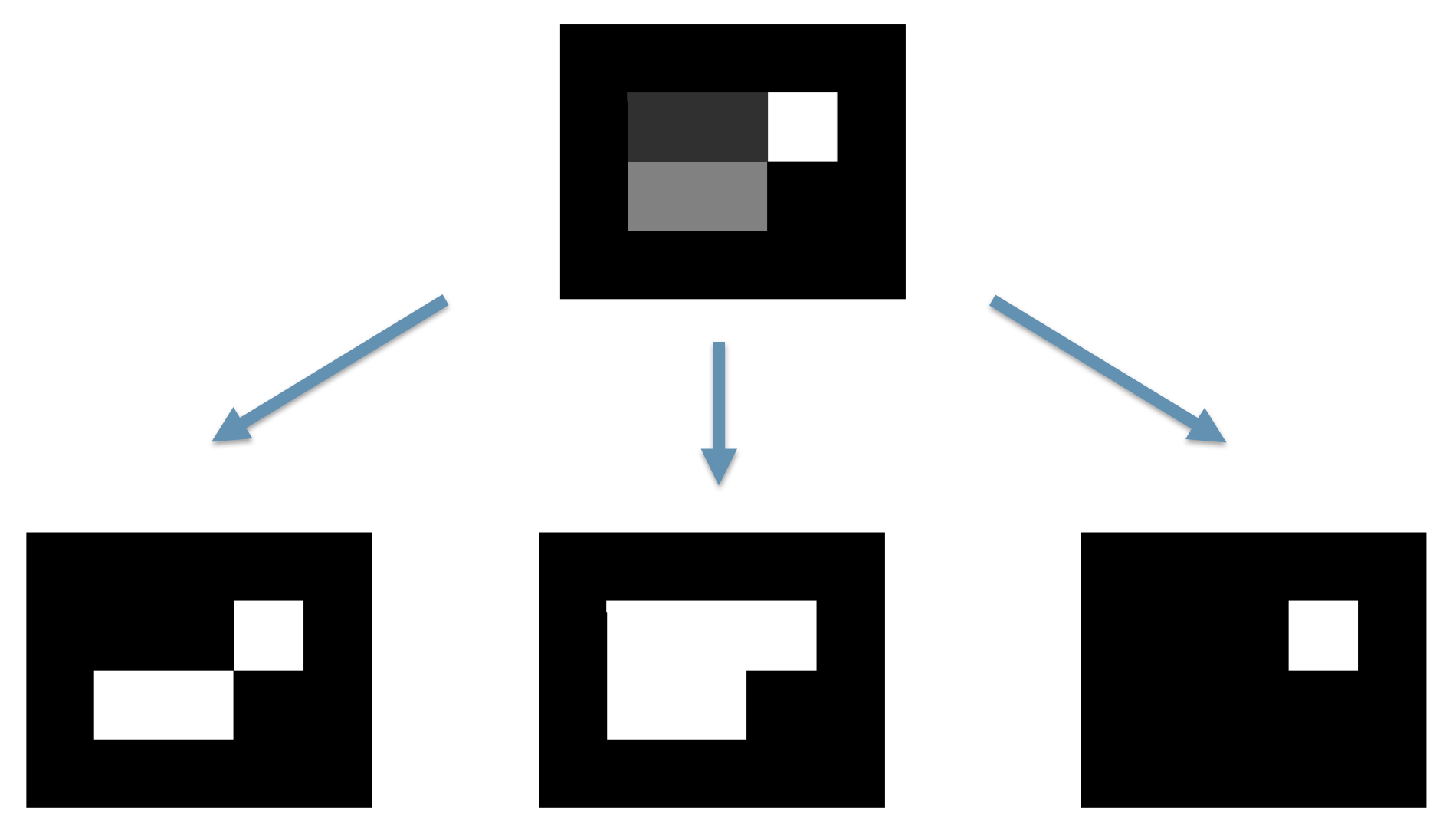
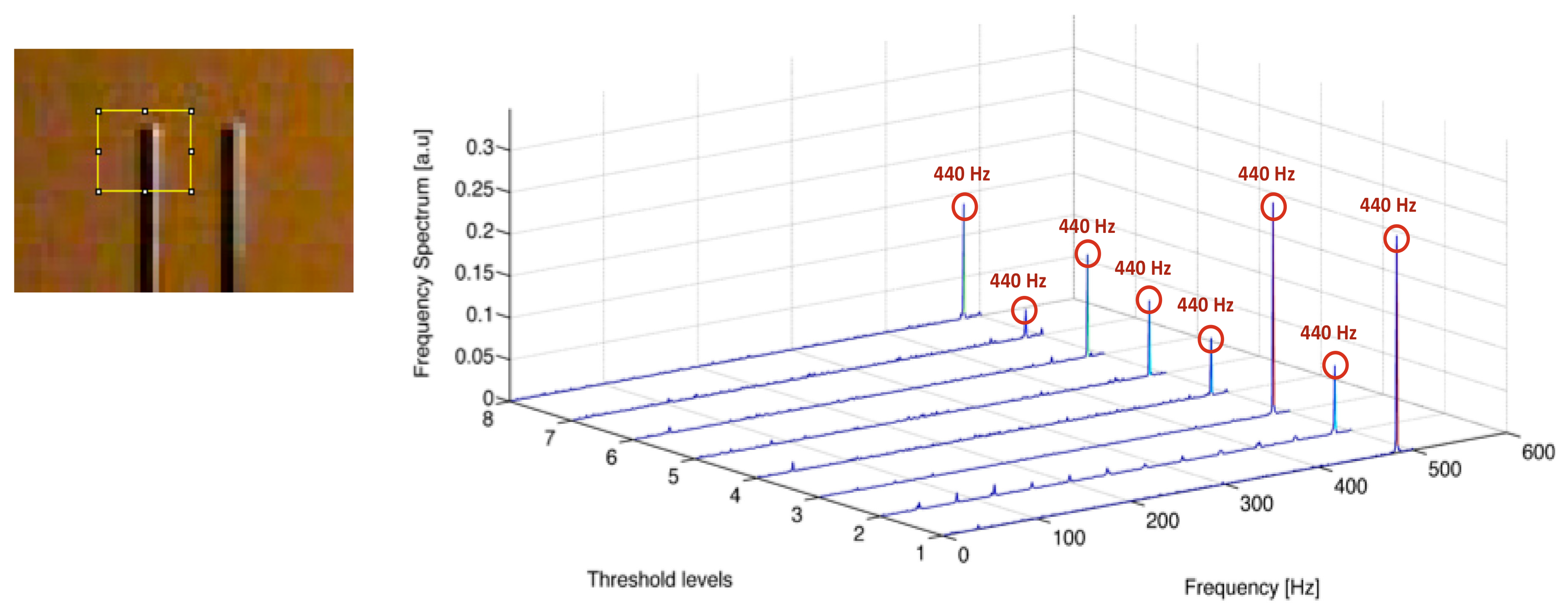
2. Image Processing Algorithm
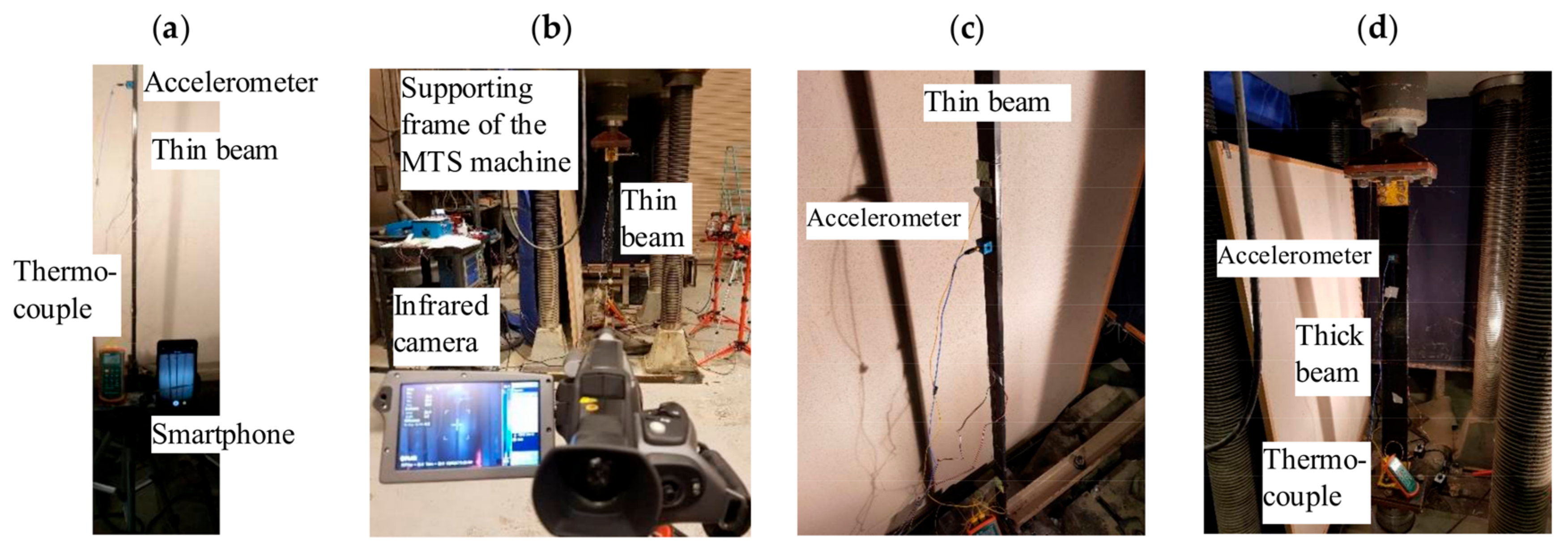
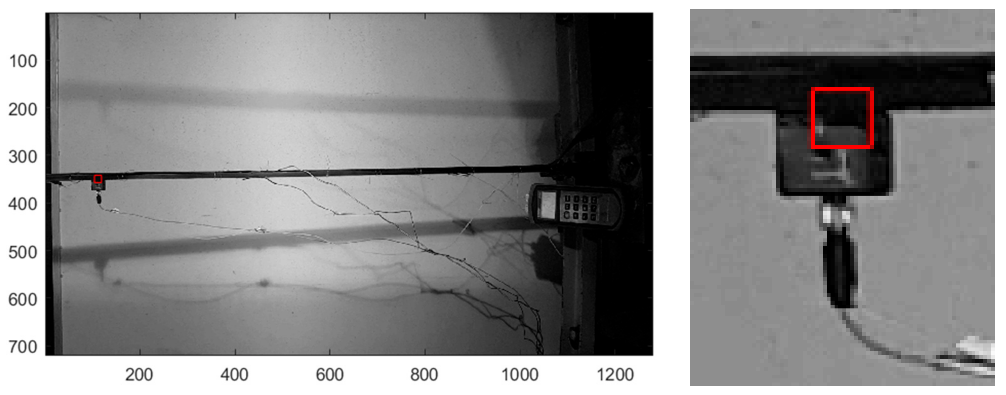
3. Experimental Setup
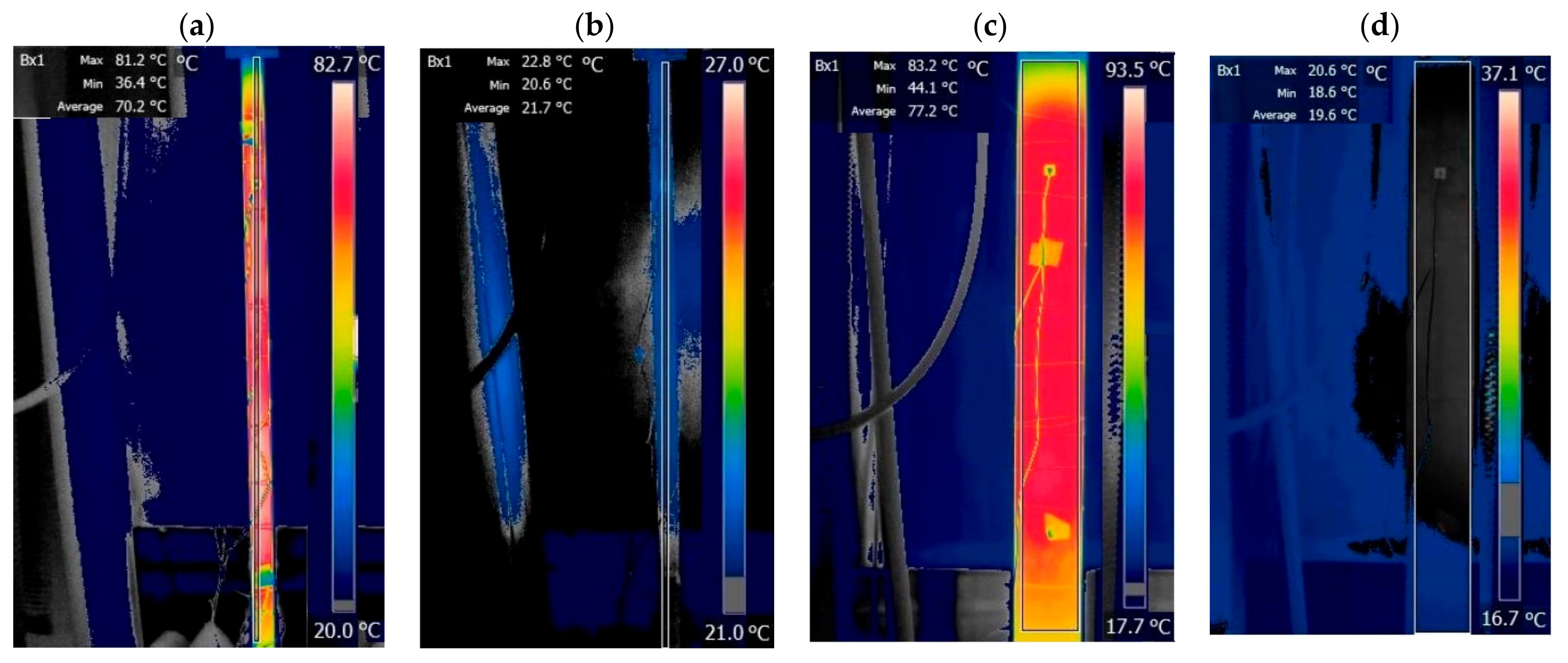
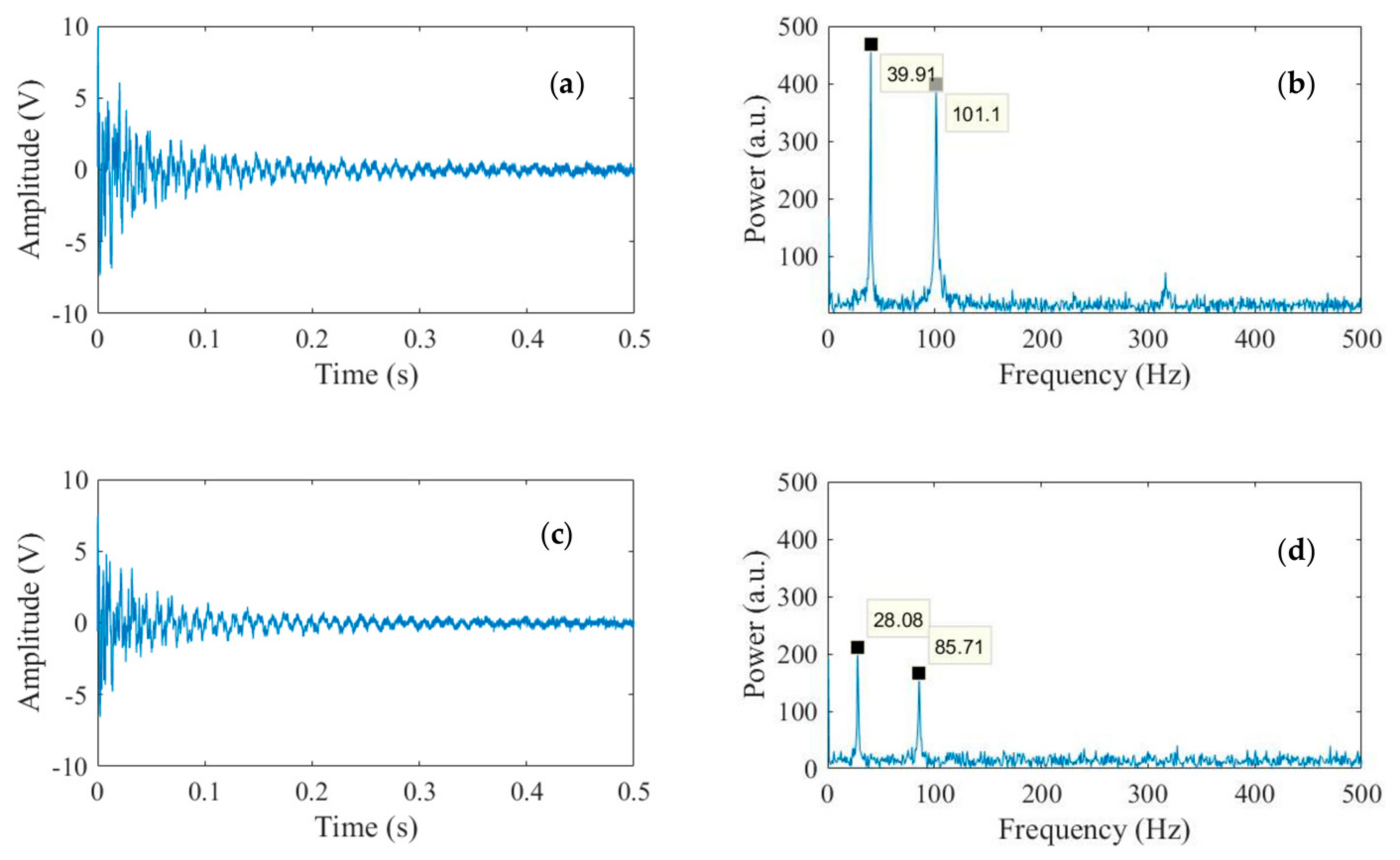
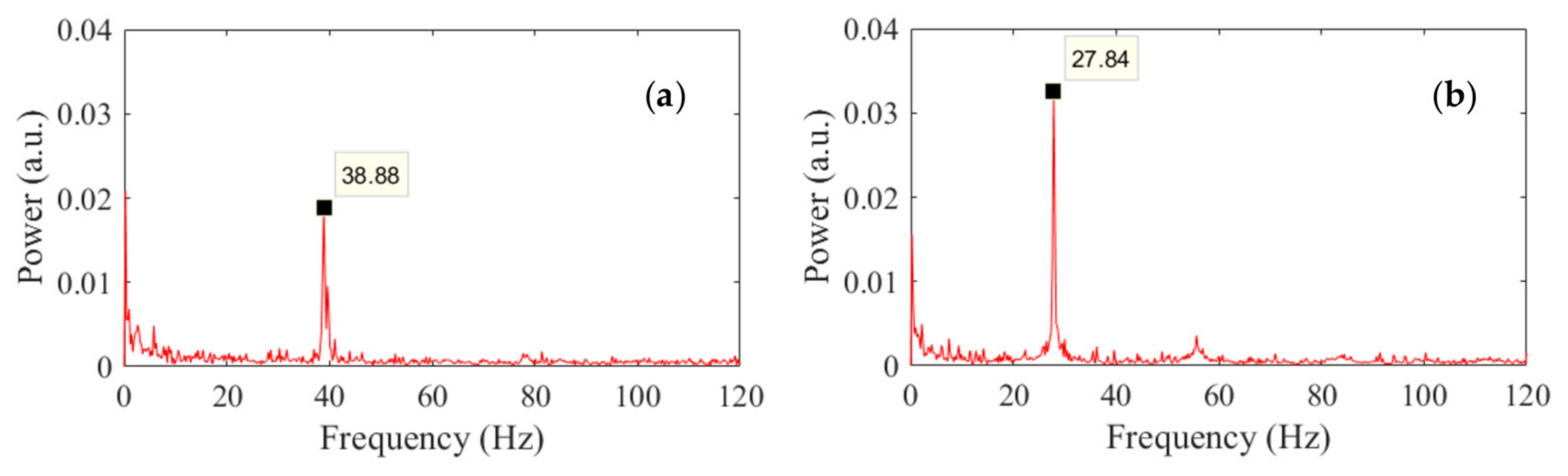
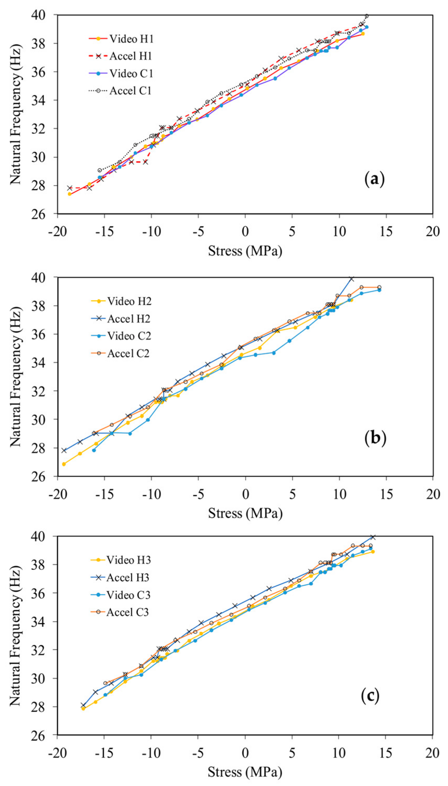
4. Results
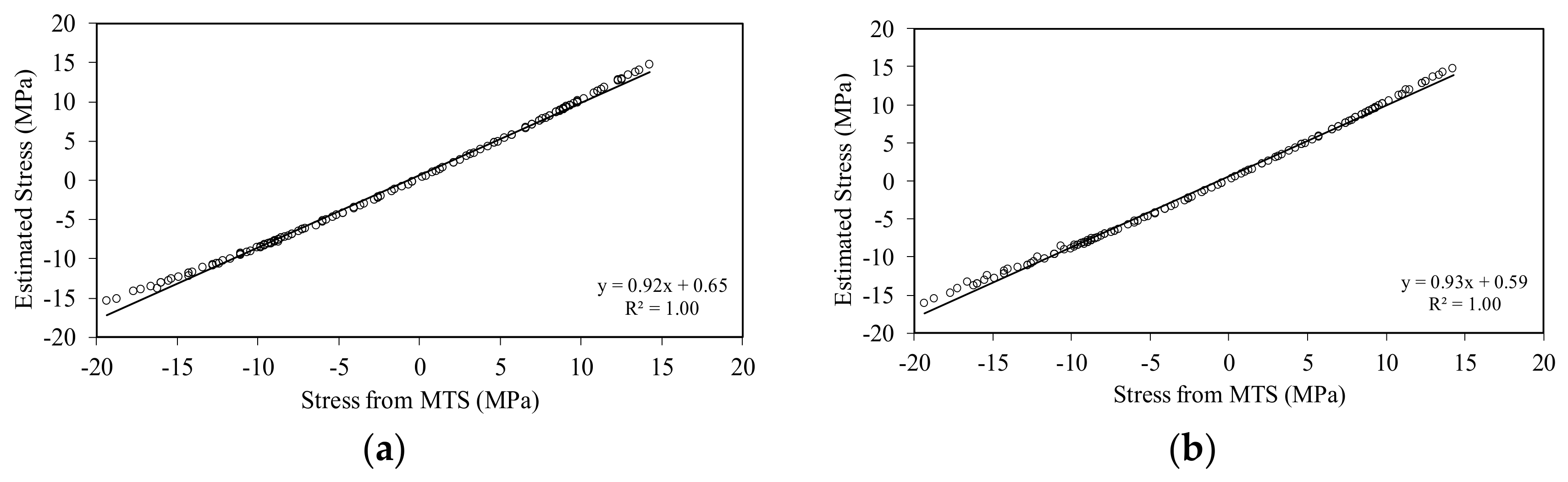
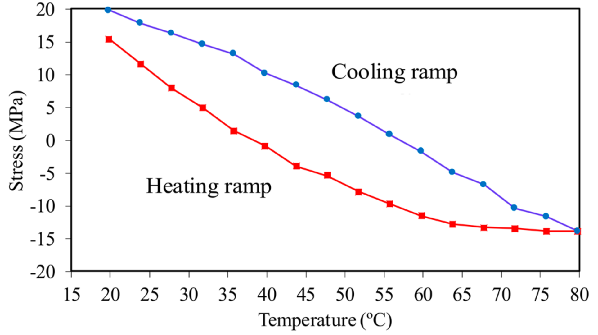
4.1. Thin Beam
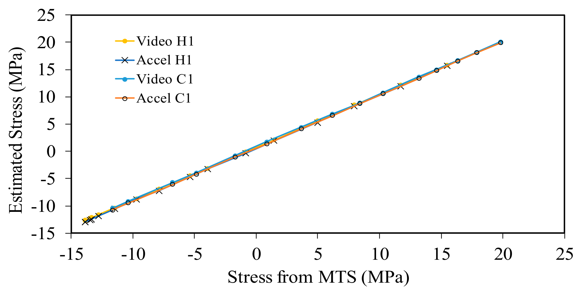
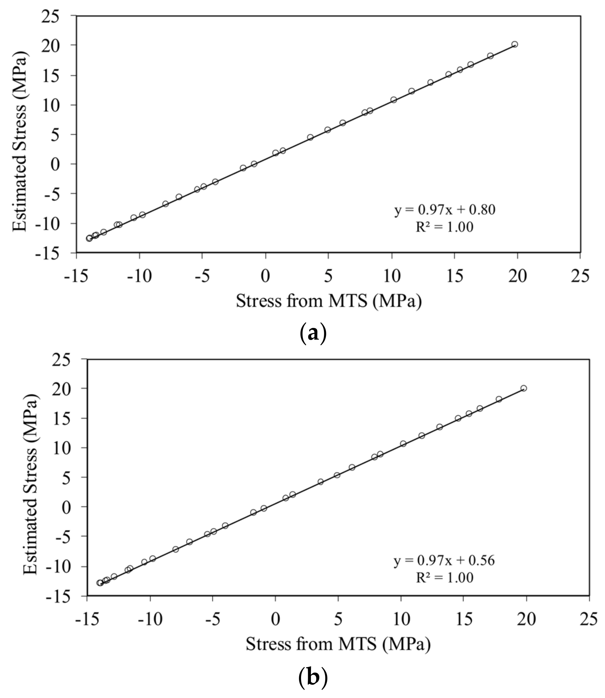
4.2. Thick Beam
5. Conclusions
Acknowledgments
Author Contributions
Conflicts of Interest
References
- Vortok International and AEA Technology. Available online: http://www.vortok.com/uploads/catalogerfiles/verse/Verse_Technical_Pack_11.07.pdf (accessed on 17 April 2018).
- Kish, A.; Samavedam, G. Longitudinal Force Measurement in Continuous Welded Rail from Beam Column Deflection Response. Am. Railw. Eng. Assoc. 1987, 88, 280–301. [Google Scholar]
- QINETIQ North America. Available online: http://www.webcitation.org/6xPqWZFdS (accessed on 22 February 2018).
- Phillips, R.; Zhu, X.; Lanza di Scalea, F. The influence of stress on Electro-mechanical impedance measurements in rail steel. Mater. Eval. 2012, 70, 1213–1218. [Google Scholar]
- Zhu, X.; Lanza di Scalea, F. Sensitivity to Axial Stress of Electro-Mechanical Impedance Measurements. Experimental Mechanics. Exp. Mech. 2016, 56, 1599–1610. [Google Scholar]
- Nucera, C.; Scalea, L.D. Nonlinear wave propagation in constrained solids subjected to thermal loads. J. Sound Vib. 2014, 333, 541–554. [Google Scholar] [CrossRef]
- Nucera, C.; Lanza di Scalea, F. Nondestructive measurement of neutral temperature in continuous welded rails by nonlinear ultrasonic guided waves. J. Acoust. Soc. Am. 2014, 136, 2561–2574. [Google Scholar] [CrossRef] [PubMed]
- Bagheri, A.; La Malfa Ribolla, E.; Rizzo, P.; Al-Nazer, L.; Giambanco, G. On the Use of L-shaped Granular Chains for the Assessment of Thermal Stress in Slender Structures. Exp. Mech. 2014, 55, 543–558. [Google Scholar] [CrossRef]
- Bagheri, A.; Ribolla, E.L.M.; Rizzo, P.; Al-Nazer, L. On the coupling dynamics between thermally stressed beams and granular chains. Arch. Appl. Mech. 2015, 86, 541–556. [Google Scholar] [CrossRef]
- Bagheri, A.; Rizzo, P.; Al-Nazer, L. Determination of the Neutral Temperature of Slender Beams by Using Nonlinear Solitary Waves. J. Eng. Mech. ASCE 2015, 141, 04014163. [Google Scholar]
- Cai, L.; Rizzo, P.; Al-Nazer, L. On the coupling mechanism between nonlinear solitary waves and slender beams. Int. J. Solids Struct. 2013, 50, 4173–4183. [Google Scholar] [CrossRef]
- Di Maio, D.; Ewins, D.J. Continuous Scan, a method for performing modal testing using meaningful measurement parameters; Part I. Mech. Syst. Signal Process. 2011, 25, 3027–3042. [Google Scholar] [CrossRef]
- Stanbridge, A.B.; Ewins, D.J. Modal testing using a scanning laser doppler vibrometer. Mech. Syst. Signal Process. 1999, 13, 255–270. [Google Scholar] [CrossRef]
- Feng, D.; Feng, M.Q. Vision-based multipoint displacement measurement for structural health monitoring. Struct. Control Health 2016, 23, 876–890. [Google Scholar] [CrossRef]
- Feng, D.; Feng, M.Q. Identification of structural stiffness and excitation forces in time domain using noncontact vision-based displacement measurement. J. Sound Vib. 2017, 406, 15–28. [Google Scholar] [CrossRef]
- Feng, M.Q.; Fukuda, Y.; Feng, D.; Mizuta, M. Nontarget vision sensor for remote measurement of bridge dynamic response. J. Bridge Eng. 2015, 20, 04015023. [Google Scholar] [CrossRef]
- Ribeiro, D.; Calçada, R.; Ferreira, J.; Martins, T. Non-contact measurement of the dynamic displacement of railway bridges using an advanced video-based system. Eng. Struct. 2014, 75, 164–180. [Google Scholar] [CrossRef]
- Cigada, A.; Mazzoleni, P.; Zappa, E. Vibration monitoring of multiple bridge points by means of a unique vision-based measuring system. Exp. Mech. 2014, 54, 255–271. [Google Scholar]
- Feng, D.; Scarangello, T.; Feng, M.Q.; Ye, Q. Cable tension force estimate using novel noncontact vision-based sensor. Measurement 2017, 99, 44–52. [Google Scholar] [CrossRef]
- Yoon, H.; Elanwar, H.; Choi, H.; Golparvar-Fard, M.; Spencer, B.F. Target-free approach for vision-based structural system identification using consumer-grade cameras. Struct. Control Health 2016, 23, 1405–1416. [Google Scholar] [CrossRef]
- Chen, J.G.; Wadhwa, N.; Cha, Y.-J.; Durand, F.; Freeman, W.T.; Buyukozturk, O. Modal identification of simple structures with high-speed video using motion magnification. J. Sound Vib. 2015, 345, 58–71. [Google Scholar] [CrossRef]
- Wadhwa, N.; Freeman, W.T.; Durand, F.; Wu, H.-Y.; Davis, A.; Rubinstein, M.; Shih, E.; Mysore, G.J.; Chen, J.G.; Buyukozturk, O.; et al. Eulerian video magnification and analysis. Commun. ACM 2016, 60, 87–95. [Google Scholar] [CrossRef]
- Cha, Y.-J.; Chen, J.; Buyukozturk, O. Motion Magnification Based Damage Detection Using High Speed Video. In Proceedings of the 10th International Workshop on Structural Health Monitoring (IWSHM), Stanford, CA, USA, 1 September 2015. [Google Scholar]
- Davis, A.; Bouman, K.L.; Chen, J.G.; Rubinstein, M.; Buyukozturk, O.; Durand, F.; Freeman, W.T. Visual Vibrometry: Estimating Material Properties from Small Motions in Video. IEEE Trans. Pattern Anal. Mach. Intell. 2017, 39, 732–745. [Google Scholar] [CrossRef] [PubMed]
- Davis, A.; Rubinstein, M.; Wadhwa, N.; Mysore, G.J.; Durand, F.; Freeman, W.T. The visual microphone: Passive recovery of sound from video. ACM Trans. Graph. 2014, 33, 1–10. [Google Scholar] [CrossRef]
- Feng, D.; Feng, M.Q. Computer vision for SHM of civil infrastructure: From dynamic response measurement to damage detection—A review. Eng. Struct. 2018, 156, 105–117. [Google Scholar] [CrossRef]
- Poozesh, P.; Sarrafi, A.; Mao, Z.; Avitabile, P.; Niezrecki, C. Feasibility of extracting operating shapes using phase-based motion magnification technique and stereo-photogrammetry. J. Sound Vib. 2017, 407 (Suppl. C), 350–366. [Google Scholar] [CrossRef]
- Chen, J.G.; Wadhwa, N.; Durand, F.; Freeman, W.T.; Buyukozturk, O. Developments with Motion Magnification for Structural Modal Identification through Camera Video. In Dynamics of Civil Structures, Proceedings of the 33rd IMAC, A Conference and Exposition on Structural Dynamics, Orlando, FL, USA, 2–5 February 2015; Caicedo, J., Pakzad, S., Eds.; Springer International Publishing: Cham, Switzerland, 2015; Volume 2, pp. 49–57. [Google Scholar]
- Gautama, T.; Hulle, M.A.V. A phase-based approach to the estimation of the optical flow field using spatial filtering. IEEE Trans. Neural Netw. 2002, 13, 1127–1136. [Google Scholar] [CrossRef] [PubMed]
- Fleet, D.J.; Jepson, A.D. Computation of component image velocity from local phase information. Int. J. Comput. Vis. 1990, 5, 77–104. [Google Scholar] [CrossRef]
- Wadhwa, N.; Rubinstein, M.; Durand, F.; Freeman, W.T. Phase-based video motion processing. ACM Trans. Graph. 2013, 32, 1–10. [Google Scholar] [CrossRef]
- Yang, Y.; Dorn, C.; Mancini, T.; Talken, Z.; Kenyon, G.; Farrar, C.; Mascareñas, D. Blind identification of full-field vibration modes from video measurements with phase-based video motion magnification. Mech. Syst. Signal Process. 2017, 85, 567–590. [Google Scholar] [CrossRef]
- Molina-Viedma, A.J.; Felipe-Sesé, L.; López-Alba, E.; Díaz, F. High frequency mode shapes characterisation using Digital Image Correlation and phase-based motion magnification. Mech. Syst. Signal Process. 2018, 102 (Suppl. C), 245–261. [Google Scholar] [CrossRef]
- Yang, Y.; Li, S.; Nagarajaiah, S.; Li, H.; Zhou, P. Real-Time Output-Only Identification of Time-Varying Cable Tension from Accelerations via Complexity Pursuit. J. Struct. Eng. 2016, 142, 04015083. [Google Scholar] [CrossRef]
- Yang, Y.; Dorn, C.; Farrar, C.; Mascarenas, D. Full-field imaging and modeling of structural dynamics with digital video cameras. In Structural Health Monitoring: Real-Time Material State Awareness and Data-Driven Safety Assurance, Proceedings of the 11th International Workshop on Structural Health Monitoring, IWSHM, Stanford, CA, USA, 2–14 September 2017; DEStech Publications, Inc.: Lancaster, PA, USA, 2017. [Google Scholar]
- Ferrer, B.; Espinosa, J.; Roig, A.B.; Perez, J.; Mas, D. Vibration frequency measurement using a local multithreshold technique. Opt. Express 2013, 21, 26198–26208. [Google Scholar] [CrossRef] [PubMed]
- Mas, D.; Ferrer, B.; Acevedo, P.; Espinosa, J. Methods and algorithms for video-based multi-point frequency measuring and mapping. Measurement 2016, 85, 164–174. [Google Scholar] [CrossRef]
- MATLAB. R2017a; The MathWorks, Inc.: Natick, MA, USA, 2017. [Google Scholar]
- Test Software and a Video Example. Available online: http://rua.ua.es/dspace/handle/10045/53429 (accessed on 17 April 2018).
- Tedesco, J.W.; McDougal, W.G.; Ross, C.A. Structural Dynamics: Theory and Applications; Addison Wesley Longman: Boston, MA, USA, 1999. [Google Scholar]
- Amba-Rao, C.L. Effect of End Conditions on the Lateral Frequencies of Uniform Straight Columns. J. Acoust. Soc. Am. 1967, 42, 900–901. [Google Scholar] [CrossRef]
- Fässler, S. Axial Load Determination Using Modal Analysis. Master’s Thesis, Lunds Tekniska Högskola, Lund, Skåne, Sweden, 2014. [Google Scholar]


| Geometric/Mechanical Properties | Thin Beam | Thick Beam |
|---|---|---|
| Steel type | 416 steel | A36 steel |
| Length (mm) | 1402 | 1395 |
| Free length L (mm) | 1207 | 1200 |
| Cross-section (mm2) | 10.12 × 41.34 | 15.88 × 127 |
| Young’s Modulus E (GPa) | 200 | 200 |
| Density ρ (kg/m3) | 7750 | 7850 |
| Poisson’s ratio v | 0.28 | 0.28 |
| Yield stress σY (MPa) | 276 | 250 |
| Coefficient of thermal expansion α (m/m°C) | 9.9 × 10⁻⁶ | 9.9 × 10⁻⁶ |
| Critical (Euler) load (kN) | 19.35 | 238.0 |
| Critical (Euler) stress (MPa) | 46.25 | 118.0 |
© 2018 by the authors. Licensee MDPI, Basel, Switzerland. This article is an open access article distributed under the terms and conditions of the Creative Commons Attribution (CC BY) license (http://creativecommons.org/licenses/by/4.0/).
Share and Cite
Sefa Orak, M.; Nasrollahi, A.; Ozturk, T.; Mas, D.; Ferrer, B.; Rizzo, P. Non-Contact Smartphone-Based Monitoring of Thermally Stressed Structures. Sensors 2018, 18, 1250. https://doi.org/10.3390/s18041250
Sefa Orak M, Nasrollahi A, Ozturk T, Mas D, Ferrer B, Rizzo P. Non-Contact Smartphone-Based Monitoring of Thermally Stressed Structures. Sensors. 2018; 18(4):1250. https://doi.org/10.3390/s18041250
Chicago/Turabian StyleSefa Orak, Mehmet, Amir Nasrollahi, Turgut Ozturk, David Mas, Belen Ferrer, and Piervincenzo Rizzo. 2018. "Non-Contact Smartphone-Based Monitoring of Thermally Stressed Structures" Sensors 18, no. 4: 1250. https://doi.org/10.3390/s18041250
APA StyleSefa Orak, M., Nasrollahi, A., Ozturk, T., Mas, D., Ferrer, B., & Rizzo, P. (2018). Non-Contact Smartphone-Based Monitoring of Thermally Stressed Structures. Sensors, 18(4), 1250. https://doi.org/10.3390/s18041250