1. Introduction
The multi-target tracking (MTT) [
1,
2] is an important capability for modern radar data processing. Taking the pulsed radar as an example, the pulse compression and clutter suppression are first used to remove clutter and jamming signals from received echoes. Then we can extract target information via integration and detection. A threshold is usually set in detection algorithms according to the Newman-Pearson discipline, and the echo signal beyond the threshold is extracted as plots. Due to the limitations of clutter suppression or detection, these plots may originate from not only targets but also clutter. Moreover, the missed detection of targets can also occur. The plots are then put into the data preprocessing (such as plots centroid, etc.) for the preparation of target tracking. The objective of MTT is to estimate the unknown and time-varying number of targets as well as their individual states from the observation sequence. It improves the radar sensing of moving targets in current search area.
The traditional multi-target tracking paradigms, such as Joint Probabilistic Data Association (JPDA) [
3] and Multiple Hypotheses Tracking (MHT) [
4], implement data association followed by the Kalman filter for single target. When targets are spatially close or a large number of false alarms are present, the data association becomes very complex. Therefore, Mahler proposes the multi-target filtering theory based on Random Finite Sets (RFS) [
5]. In the framework of this theory, multi-target states and sensor measurements are modeled as random finite sets, and the recursive estimation of multi-target posterior density is achieved by Bayesian multi-target filtering. The early implementations of RFS paradigm, such as probability hypothesis density (PHD) [
6], cardinalized probability hypothesis density (CPHD) [
7] and Multi-Bernoulli [
8] filters, ignore the data association in order to reduce the computational complexity. Hence they cannot produce target tracks. On the basis, δ-generalized labeled Multi-Bernoulli (δ-GLMB) [
9,
10] and labeled Multi-Bernoulli (LMB) [
11] filters incorporate track labels into target state and take data association as part of multi-target state estimation to realize the output of target tracks.
The traditional radar signal processing procedure is first detection and then tracking. Nevertheless, when the detection performance is unsatisfactory, the tracking accuracy will decline. In this case, the track-before-detect (TBD) strategy [
12,
13,
14,
15,
16] is proposed. It gets rid of the detection in any single frame, but accumulates the likelihood ratio of continuous multiple frames. This strategy provides an effective way for detecting low observable targets. It should be noted that the tracking also carries out likelihood ratio accumulation, and the difference between them is: (1) the likelihood ratio accumulated by TBD approaches contains both dynamic states and amplitude information (AI) of the target, while the tracking approaches only contains the dynamic states; (2) TBD deals with the original echoes, and traverses all range-Doppler-azimuth cells over the observation area, while the tracking only needs to process the data after thresholding. Thus, more information amount and computational burden are involved in the TBD. This disadvantage leads to the fact that TBD is currently difficult to replace the traditional detection-and-tracking procedure in real-time radar data processing. However, it outperforms the traditional procedure in low signal-to-clutter-ratio (SCR) conditions due to the full use of amplitude difference between target and clutter. Therefore, we can see that the tracking performance in low SCR conditions could be improved by using AI.
Many works in the literature have introduced AI into tracking algorithms. In [
17], the detection process of echoed signals with slow Rayleigh fluctuation in narrowband Gaussian background is analyzed. It incorporates the likelihood ratio of amplitude into the calculation of measurement-track association weights for improving performance of the tracking filter. Based on the AI aided measurement-track association (AIA-MTA) approach in [
17], more studies have further been carried out. In [
18], Lerro combines the AIA-MTA with the interactive multiple model (IMM), and improves the performance of track formation and maintenance in clutter environment. To solve the track initiation problem of low observable target, Cai introduces AI into the adaptive sliding window expectation-maximization algorithm combined with maximum likelihood [
19]. By analytically assessing the benefits of AIA-MTA in several simple cases, Ehrman points out that the method is unsuitable for multiple targets although it is good at tracking single target in dense clutter environment. The reason is that AIA-MTA always favors the measurement with high amplitude, but ignores the measurement states [
20]. Then he proposes that the normalized target amplitude likelihood function instead of the likelihood ratio should be introduced into AIA-MTA. In [
21], the error probabilities of measurement-track association for Rayleigh target, fixed amplitude and Rician target are calculated. In [
22,
23], Ehrman further presents that the blind use of AI in the measurement-track assignment may actually reduce the association performance, because no method can be applied to all scenarios. In [
24], the performance loss in heavy-tailed clutter environment is analyzed quantitatively by simulation. In [
25], a modified Riccati equation is used to predict the performance of probabilistic data association filter with AI in heavy-tailed K distributed clutter. In [
26,
27], the amplitude likelihood ratio proposed in [
17] is introduced to the PHD filter (simplified as PHD-AI). For situations of high resolution and low grazing angle, an AI assisted PHD filter in Weibull clutter background is proposed by Li [
28]. In [
29], Liu proposes to improve the association performance with AI in complex ground target tracking. In [
30], Yuan gives an improved multi-Bernoulli filter with AI.
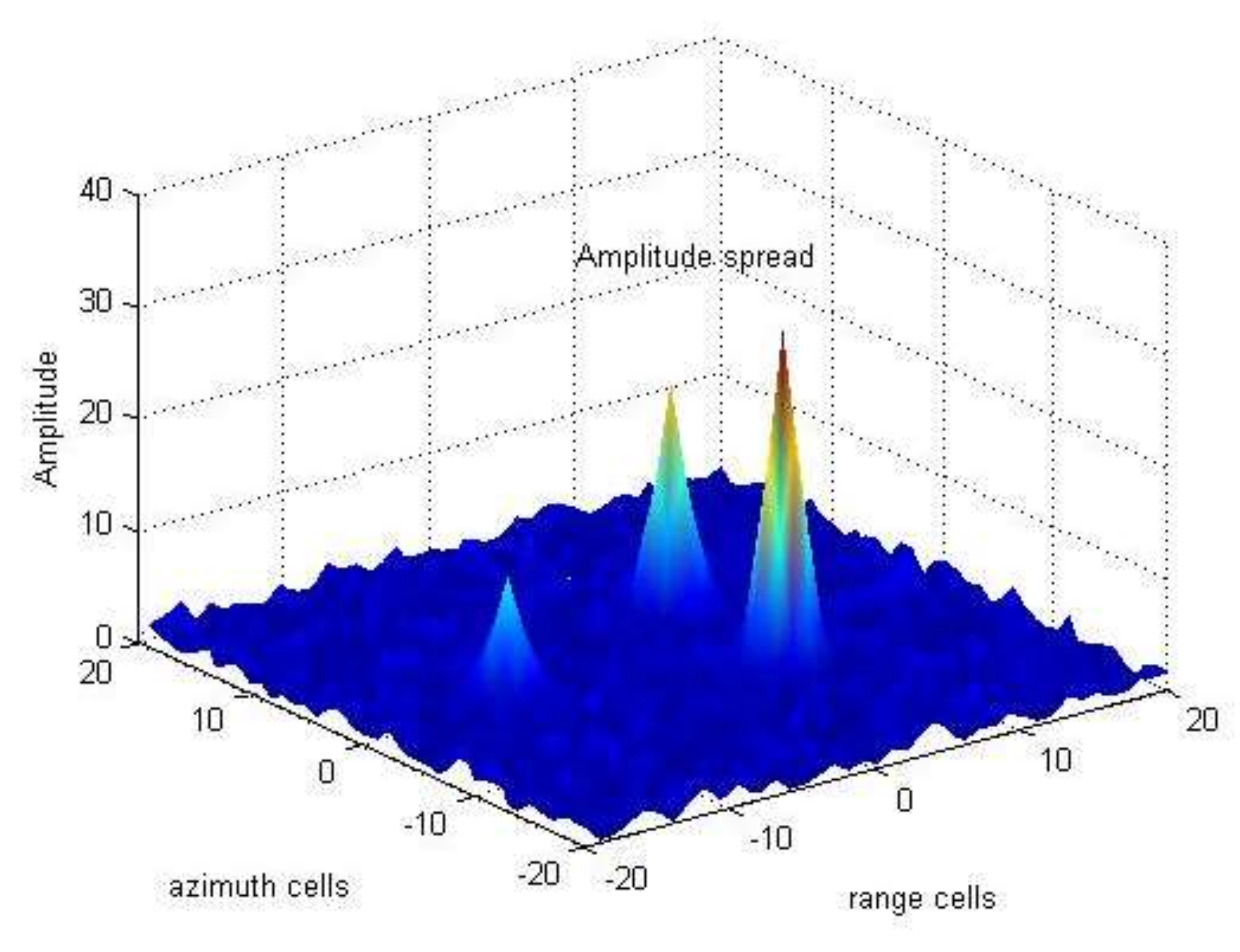
However, one obvious disadvantage of these existing researches is that when constructing, only the AI of the measurement cell is used for constructing the amplitude likelihood function, while that of surrounding cells is ignored. In some cases, for example, when the size of the target is large or the sampling interval of range and azimuth is small, the target echoes may occupy multiple adjacent cells. After detection process, the plots are likely to be distributed in multiple adjacent cells. This phenomenon is called spread [
12] or spillover [
16] of target energy. In order to reduce complexity, most of target tracking approaches require that one measurement is generated for a target in each frame [
5]. Therefore, the plots centroid technology is usually applied to handle the neighboring plots, and a central measurement is obtained according to certain principles. The central measurement would be used as the only target measurement for tracking, while the other neighboring plots are discarded. If AI of surrounding cells is preserved at the step of plots centroid, the amount of available information for filtering will be greatly increased. It could help improve the tracking performance. By now, this idea has been used in some TBD approaches [
12,
13,
16].
Based on the above analysis, this paper proposes a new δ-GLMB filter with united likelihood ratio of AI in neighboring cells in the complex Gaussian distributed clutter (simplified as GLMB-AI-UL). First, using PHD-AI [
27], a δ-GLMB filter with single cell AI (simplified as GLMB-AI) is derived. Then the amplitude measurement is modeled with the point spread function employed in TBD approaches. However, different from traversing all cells in TBD to calculate the amplitude likelihood ratio, the method only considers cells around each measurement after plots centroid to obtain the likelihood ratio. Thus, its calculation cost is significantly lower than that of TBD. Finally, the likelihood ratio is introduced into δ-GLMB update process and measurement-track assignment cost matrix to improve its filtering performance.
The remainder of this paper is organized as follows. A brief overview of RFS and the δ-GLMB filter are provided in
Section 2. PHD-AI is introduced in
Section 3. On this basis the GLMB with united likelihood ratio of AI in neighboring resolution cells is proposed in
Section 4.
Section 5 presents simulation results. Conclusions are made in
Section 6.
5. Simulations
In this paper, the performance of GLMB-AI-UL is compared with that of other two algorithms, i.e., GLMB-AI and δ-GLMB (simplified as GLMB), by simulation data in three SCR scenarios.
Table 2 shows the specific parameter settings.
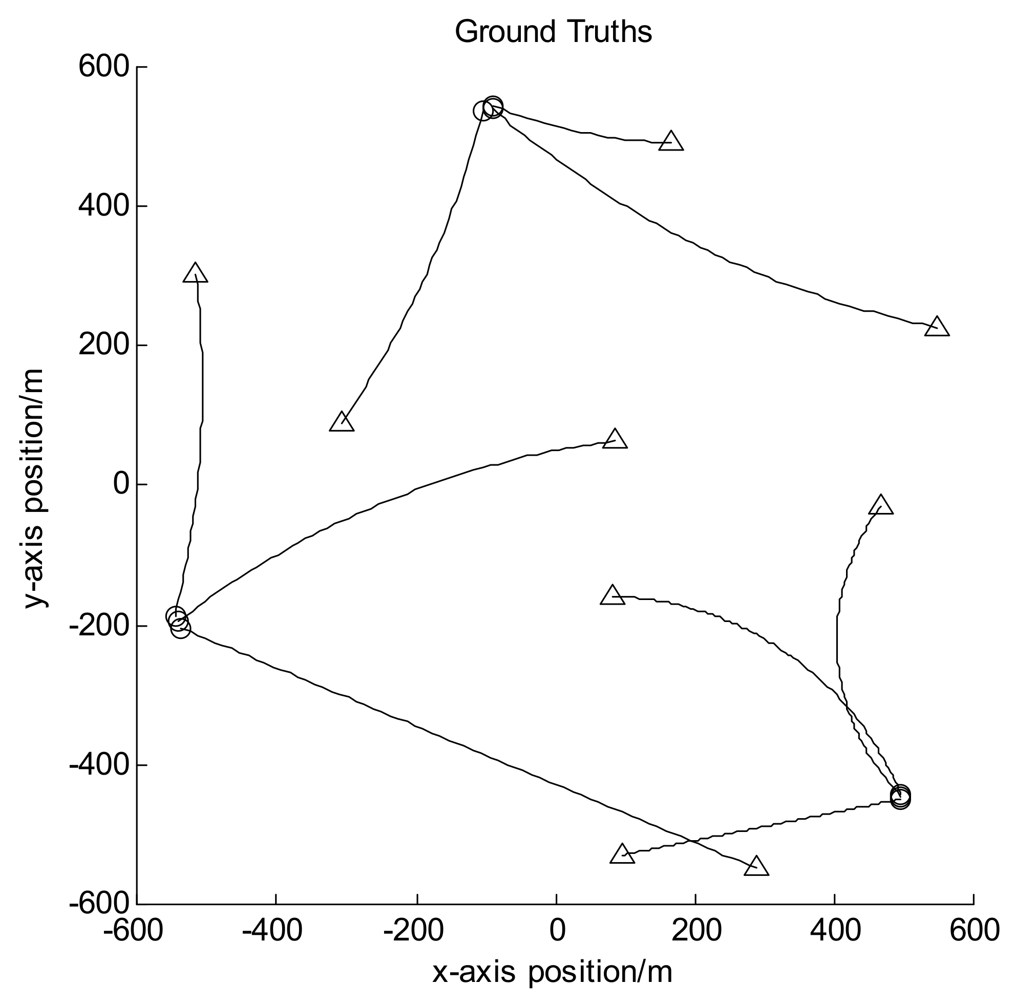
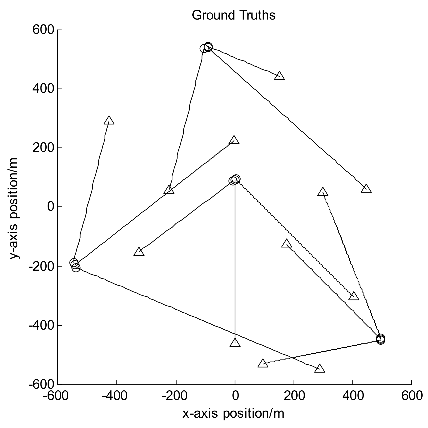
Let the size of observation area be [−600, 600] m × [−600, 600] m, and the observation period be 100 frames in all. In scenarios 1 and 2, there are 12 moving targets following the nearly-constant-velocity (NCV) model, and their trajectories are shown in
Figure 2; while in scenario 3, there are 9 targets with some of them following the coordinated turn (CT) model, and their trajectories are shown in
Figure 3. In both figures the circles denote the starting points of the target trajectories while the triangles denote corresponding endpoints, and each target has different appearance and disappearance time. Hence the target number is varying in each frame. Set the clutter number before detection to be Poisson distributed with the mean value of 800. It can be seen that after detection it is also Poisson distributed with the mean value of about 80. For GLMB without AI, the survival probability is set to be 0.9 and the detection probability to be 0.95. For GLMB-AI-UL and GLMB-AI, the survival probability is set to be 0.9, and the detection probability can be calculated by Equations (16) and (17) according to the SCR and false alarm probability.
To evaluate the performance of GLMB-AI-UL, all the targets are simulated to spread their amplitude to neighboring cells. Due to the Rayleigh amplitude distribution, each target has different amplitude, and accordingly its spread scope is distinct as well. For the convenience of calculation, parameters of the point spread function in Equation (33) is set to be
. When calculating AI-UL with Equations (50) and (51), only the neighbor cells next to any central measurement are considered. The OSPA metric [
31] is used to evaluate the performance of three multi-target tracking algorithms mentioned above, which is defined as follows
where we set
and
in simulations. In each scenario, we make 20 Monte Carlo runs for the three algorithms, and their performance are compared and analyzed by calculating the mean error.
5.1. Results of Scenario 1
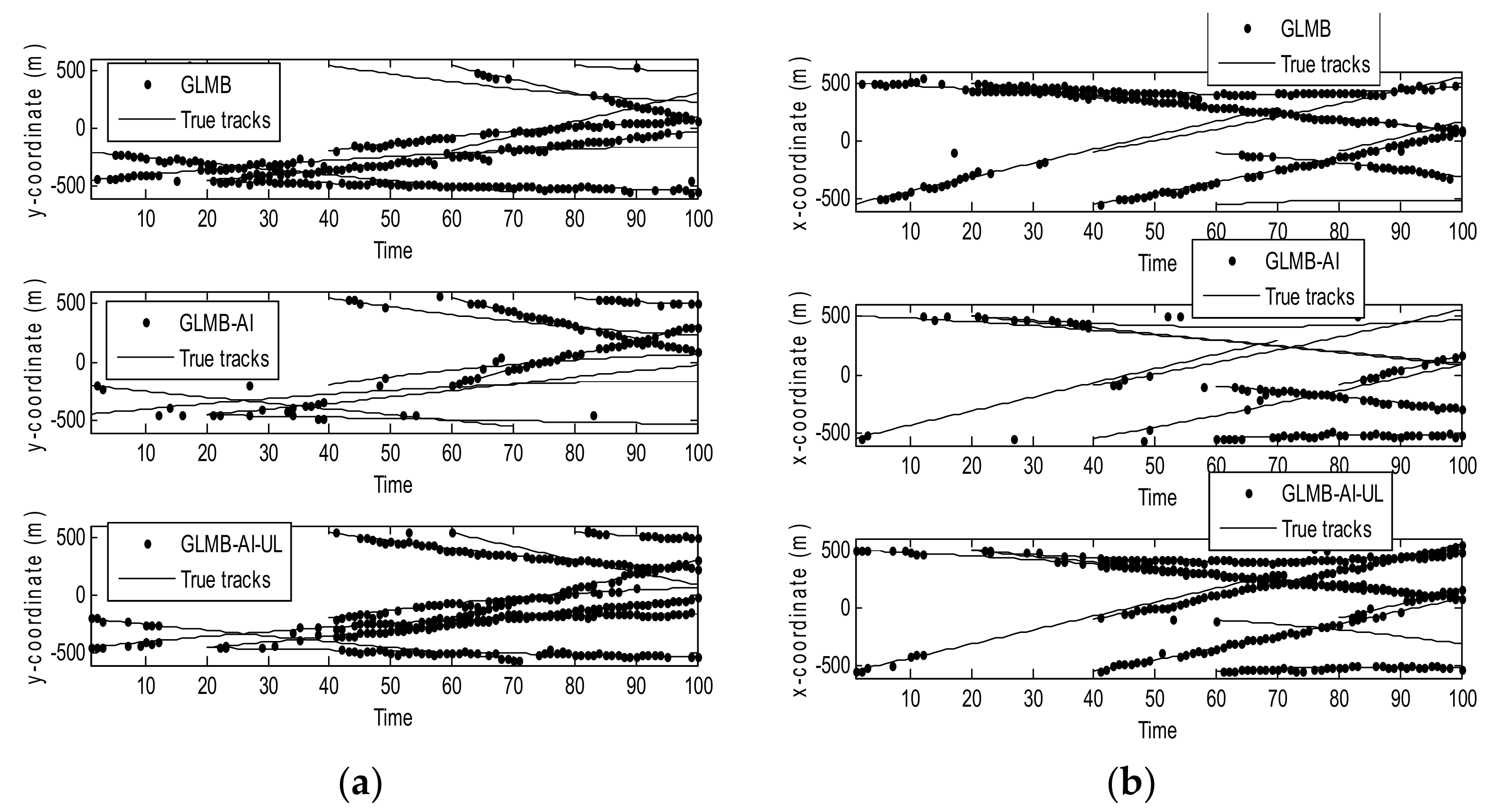
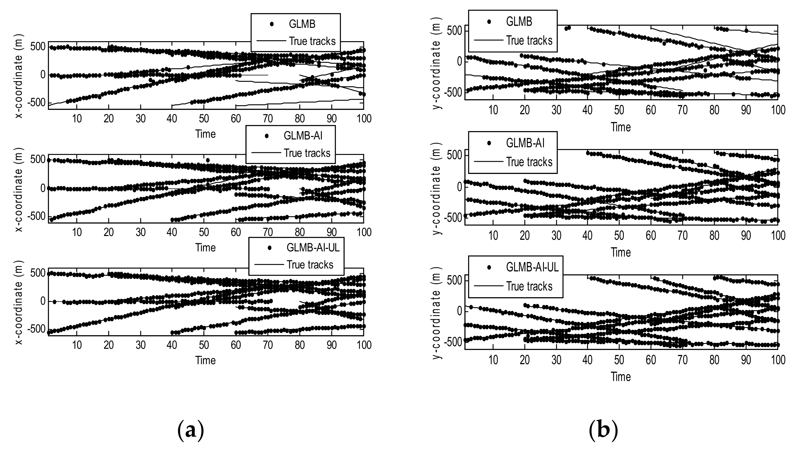
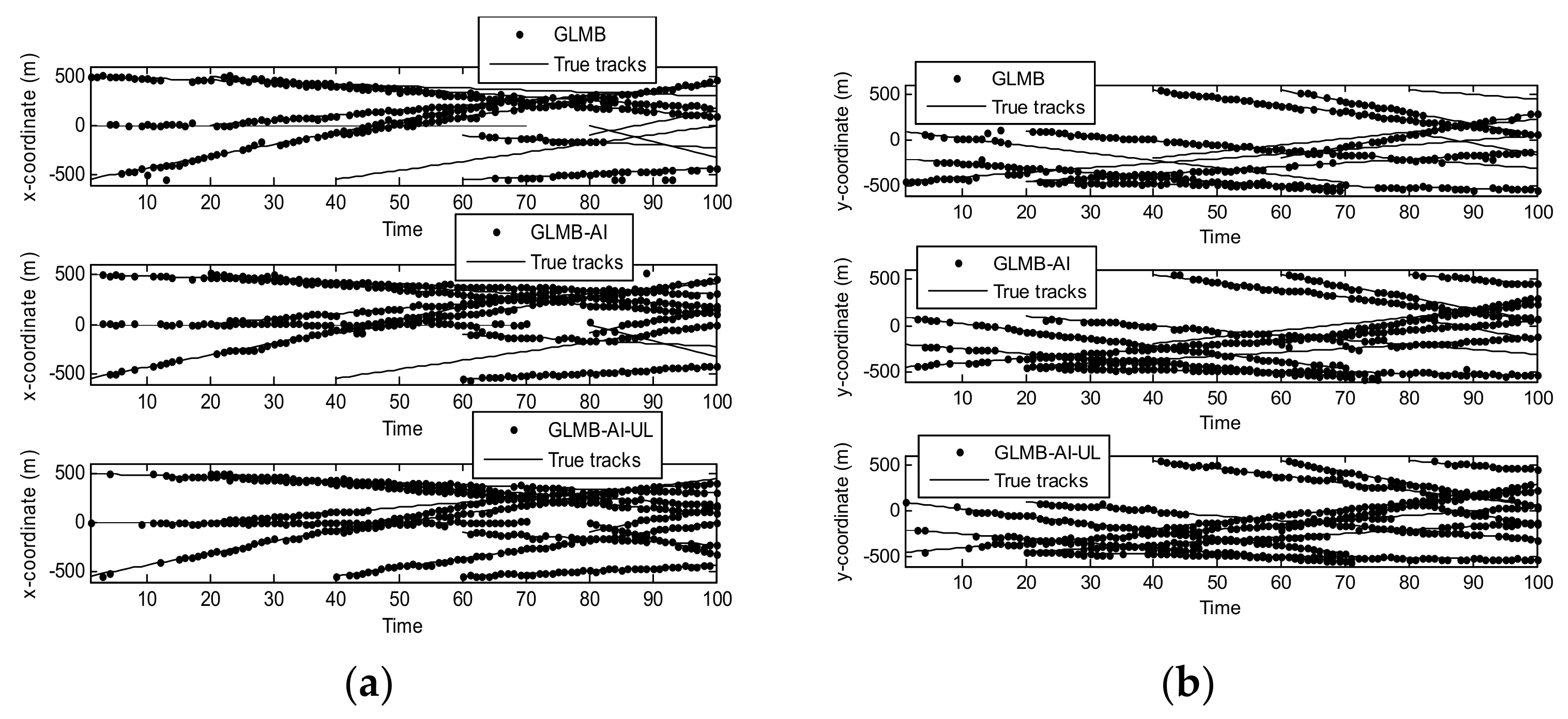
Figure 4 shows the filtering output of the three algorithms in a single operation, where
Figure 4a shows the true and estimated positions in x coordinate, while
Figure 4b shows the true and estimated positions in y coordinate. As can be seen that the GLMB produces some missed tracks and false tracks, while the two filters using amplitude information, i.e., the GLMB-AI and GLMB-AI-UL give much more accurate estimates.
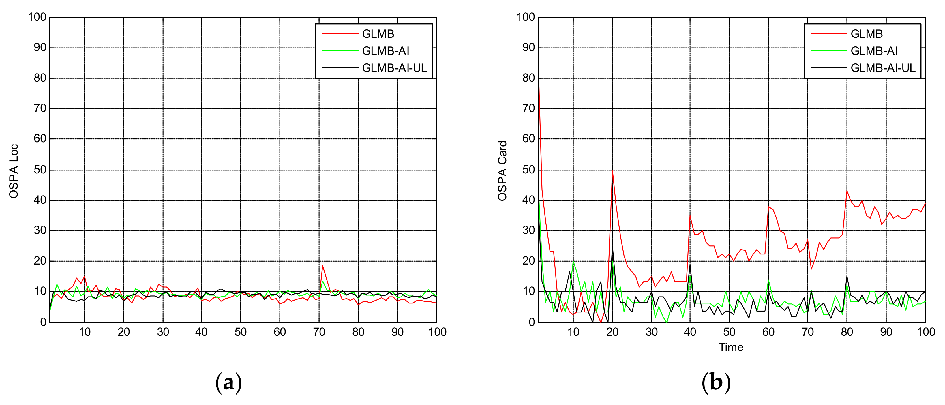
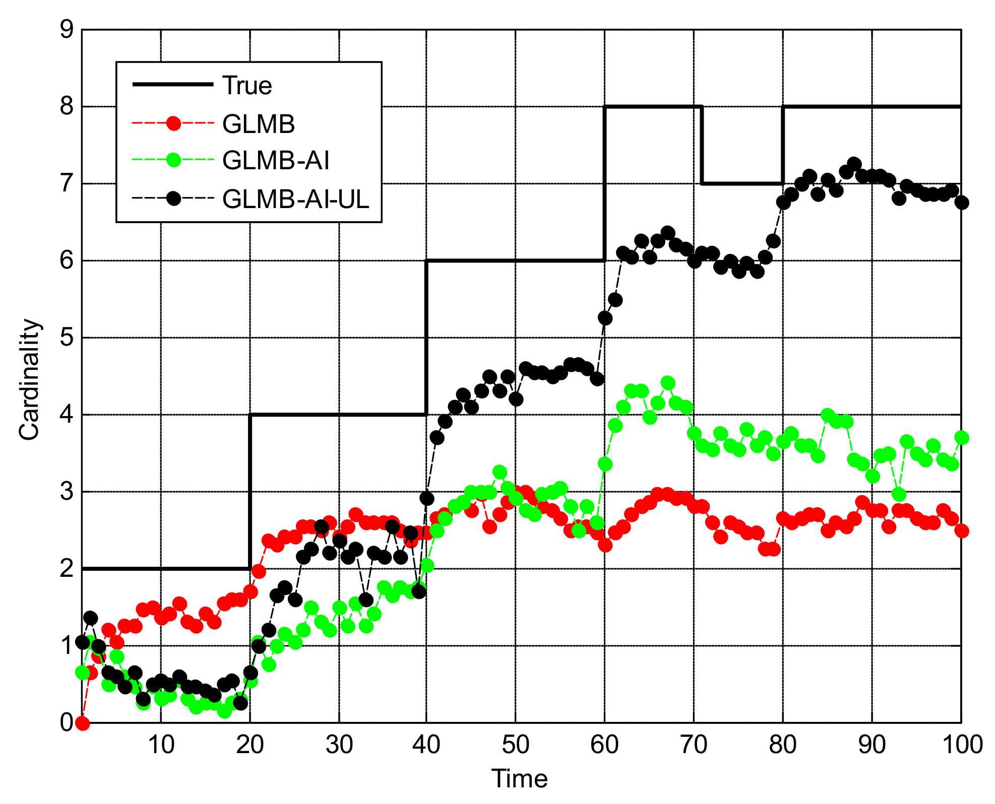
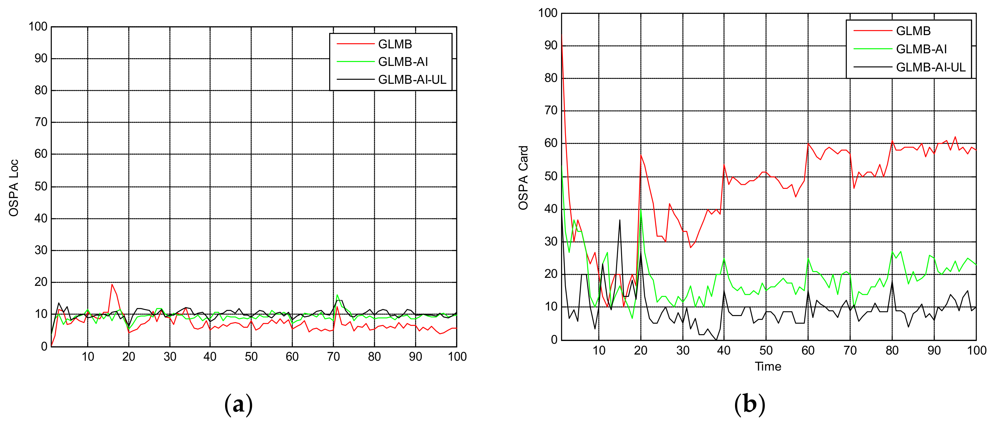
Figure 5 shows the OSPA miss distance and
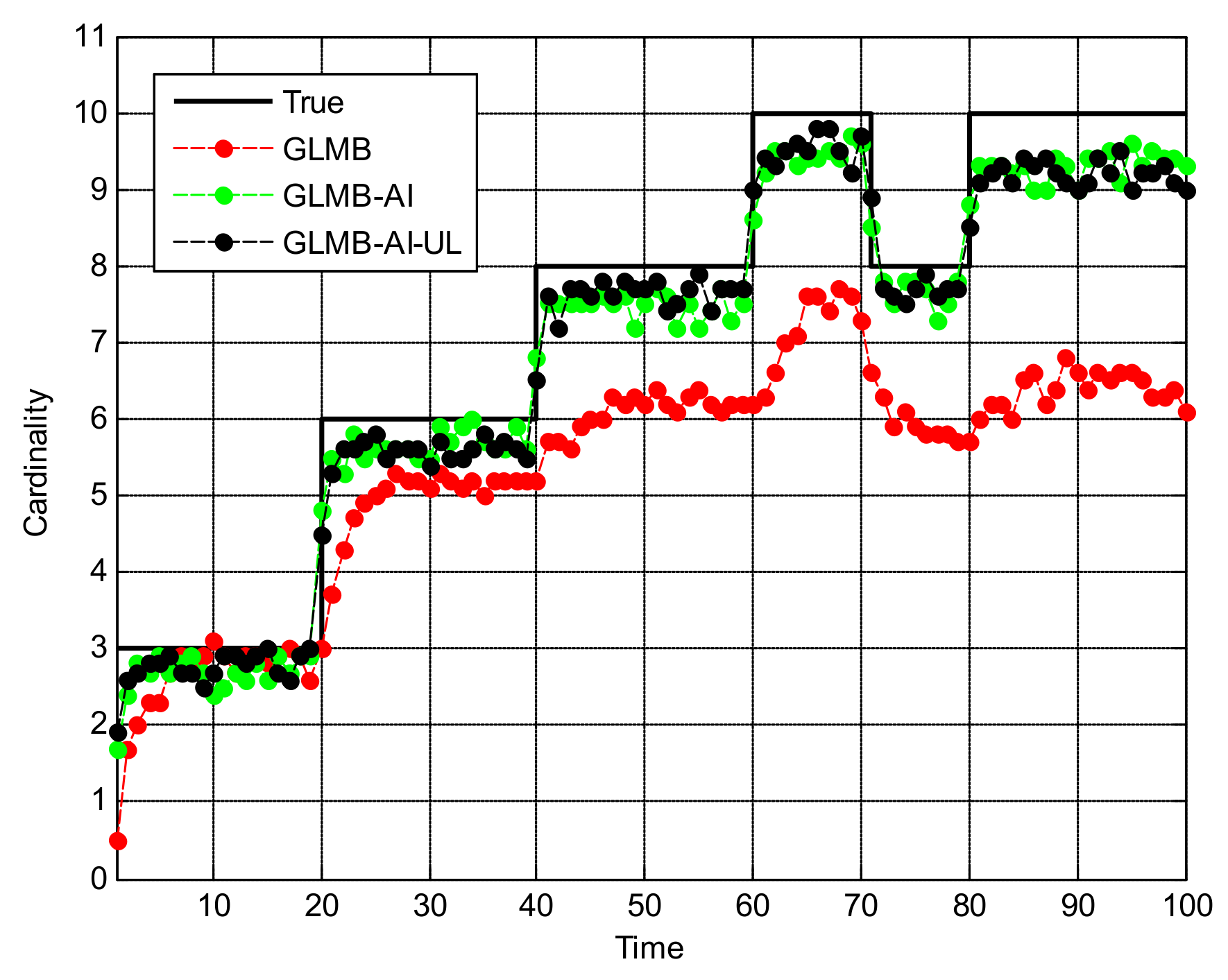
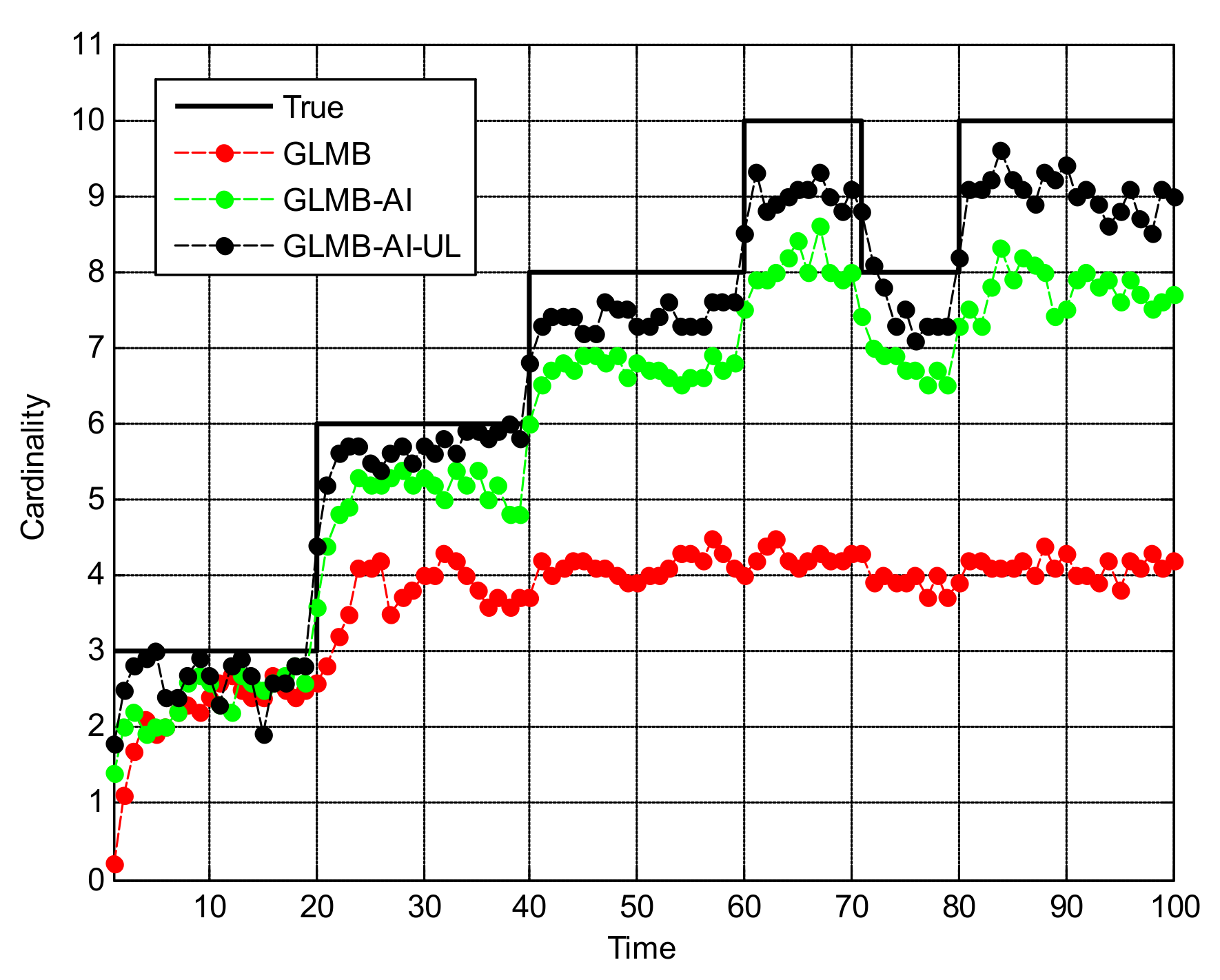
Figure 6 shows the comparison of cardinality estimates, and both are averaged over 20 trials. We can see from
Figure 5a that the state estimation performance of GLMB-AI-UL and GLMB-AI are similar to that of the standard GLMB which only uses target dynamic information, and even at some times the GLMB performs slightly better than the GLMB-AI-UL and GLMB-AI. A possible reason for this result is that the cardinality error is ignored when calculating the location error of OSPA, which has been further discussed in [
27]. GLMB may generate some false tracks due to a poorer association performance, and these tracks may be close to the actual ones of targets in space, which results in a smaller estimation error. However, in terms of the cardinality estimation performance shown in
Figure 5b and
Figure 6, GLMB-AI-UL and GLMB-AI are significantly better than GLMB. This is due to the exploitation of amplitude information for calculating the measurement to track association weight in the first two algorithms. In this scenario, the cardinality estimation performance of GLMB-AI-UL is almost same as that of GLMB-AI. The most possible reason for the similarity is that the SCR is high enough for GLMB-AI to distinguish target from clutter.
5.2. Results of Scenario 2
Figure 7 shows the filtering output of the three algorithms in a single run in x coordinate and y coordinate respectively. Compared with
Figure 3, it can be seen that with the decrease of SCR, the state estimation performance of the three algorithms is significantly reduced. In particular, the GLMB generates more missed tracks and false tracks, and the GLMB-AI also produces some missed tracks and false tracks. Although the GLMB-AI-UL lost some plots, it still gives the most accurate state estimation, because by taking advantage of the energy of the surrounding units, a more efficient likelihood accumulation is realized.
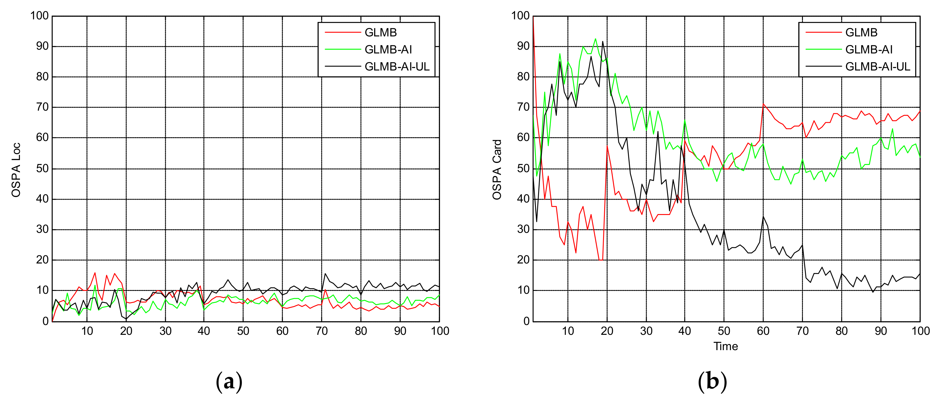
Figure 8 and
Figure 9 are the comparison of averaged tracking results in scenario 2. As can be seen from
Figure 8a, the state estimation performance of the three algorithms is quite similar to that of scenario 1, and the superiority of GLMB is more obvious. This is because when the SCR is lower, GLMB may produce more false tracks, which can be closer to the target.
Figure 6 and
Figure 8b show that the performance of cardinality estimation of GLMB-AI-UL and GLMB-AI is still significantly better than that of GLMB. However, different from scenario 1, the performance of GLMB-AI-UL is obviously better than that of GLMB-AI. The potential reason is that it is difficult to distinguish the target from clutter only by the amplitude characteristics of a single unit when the SCR is low. Nevertheless, it is possible to improve the differentiation ability by using the combined likelihood ratio of multiple resolution cells. In scenarios 1 and 2, we can also see that when the SCR is low, the deterioration degree of GLMB is the largest, and followed by GLMB-AI, which uses only single unit amplitude information, whereas GLMB-AI-UL with AI of multiple units is the most robust to strong clutter.
5.3. Results of Scenario 3
Figure 10,
Figure 11 and
Figure 12 are the comparison of tracking results in scenario 3. Unlike the previous two scenarios, the motion of targets in this scenario is no longer linear, but rather maneuvering, and the SCR is set with a very low value of 8 dB.
From
Figure 10 we can see that in this scenario, the tracking performance of the three algorithms is significantly reduced, and many missed tracks and false tracks are generated, but the GLMB-AI-UL still outperforms the other two algorithms, which proves the validity of the proposed method once again. From
Figure 11b and
Figure 12 we can see that except for the initial 40 frames, the cardinality estimation performance of the GLMB-AI-UL is always the best in the rest of the filtering time.
Table 3 is the average running time of each algorithm in the three scenarios. As can be seen from this table, in scenario 1, when the SCR is relatively high, the filtering performance of GLMB is good, and its calculation speed is the highest. This is because the calculation of amplitude information results in an increase in computational cost. However, when the SCR was reduced, in scenario 2, the GLMB’s running time is only slightly reduced, but the elapsed time of the latter two algorithms with amplitude information is greatly reduced. This is because as the SCR decreases, the number of target-generated measurements decreases, and the utilization of amplitude information enhances the computational efficiency of the measurement-track assignment matrix. When the SCR is further reduced, the running time of the proposed GLMB-AI-UL continues decreasing, but that of the GLMB and GLMB-AI increase a lot, and the GLMB-AI-UL outperforms the other two algorithms in terms of computational cost. A reasonable explanation for this phenomenon is that, in this scenario, the SCR is such low that only few target-generated measurements exceed the threshold. This will reduce the computational cost on one hand, but on the other hand, the low SCR leads to a poorer computational efficiency of the measurement-track assignment matrix for the GLMB and GLMB-AI. Especially, the exploitation of amplitude information only of a single unit is less effective, which results in a poor performance for GLMB-AI, even worse than that of GLMB without using amplitude information. However, using the amplitude information of multiple adjacent units can evidently improve the performance. Thus, the proposed method is of great value in practical radar applications, especially when the SCR is very low.
The simulations of this paper are carried out with Matlab, and the proposed algorithm seems time consuming. However, if the procedure is written in C language, the running time will be greatly reduced. Therefore, this algorithm is suitable for real-time radar applications, particularly for low SCR environments.


