3D Laser Scanner for Underwater Manipulation

 , , , , and
Abstract
:1. Introduction
2. Related Work
3. Mechatronics
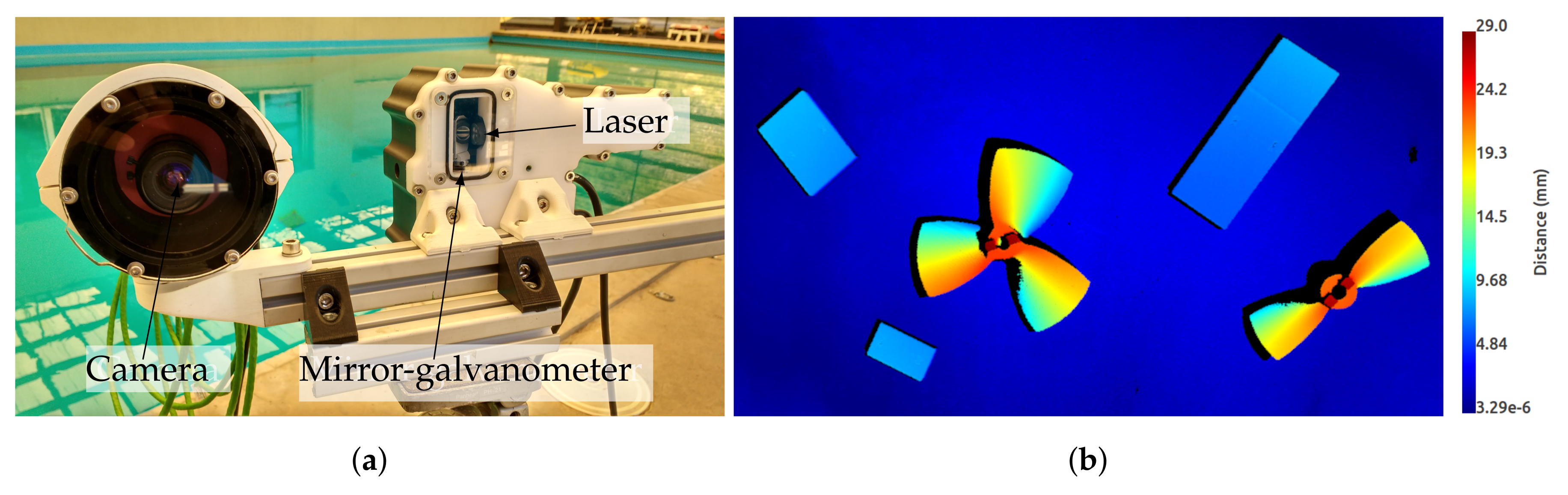
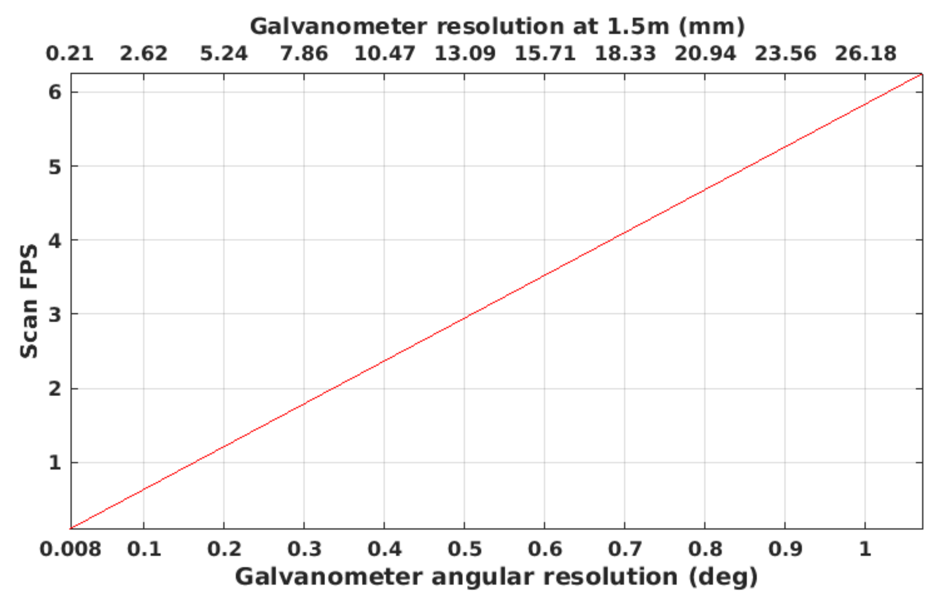
3.1. Laser Scanner
3.2. Fixed-Based Underwater Manipulator System
3.2.1. Cartesian Manipulator
3.2.2. 6 DoF Robotic Arm
3.3. Underwater Vehicle Manipulator System
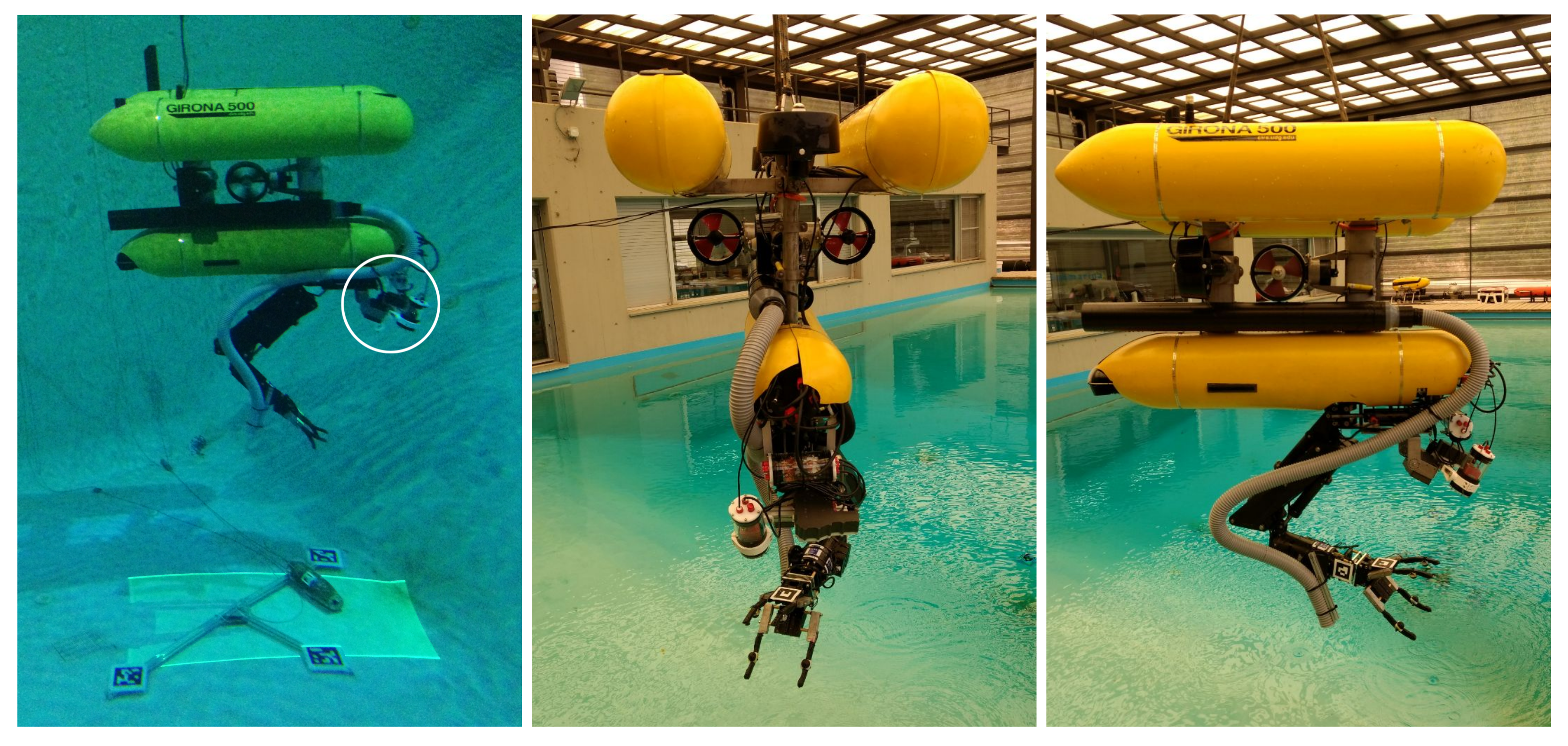
3.3.1. Girona 500 AUV
3.3.2. Four DoF Robotic Arm
4. Calibration
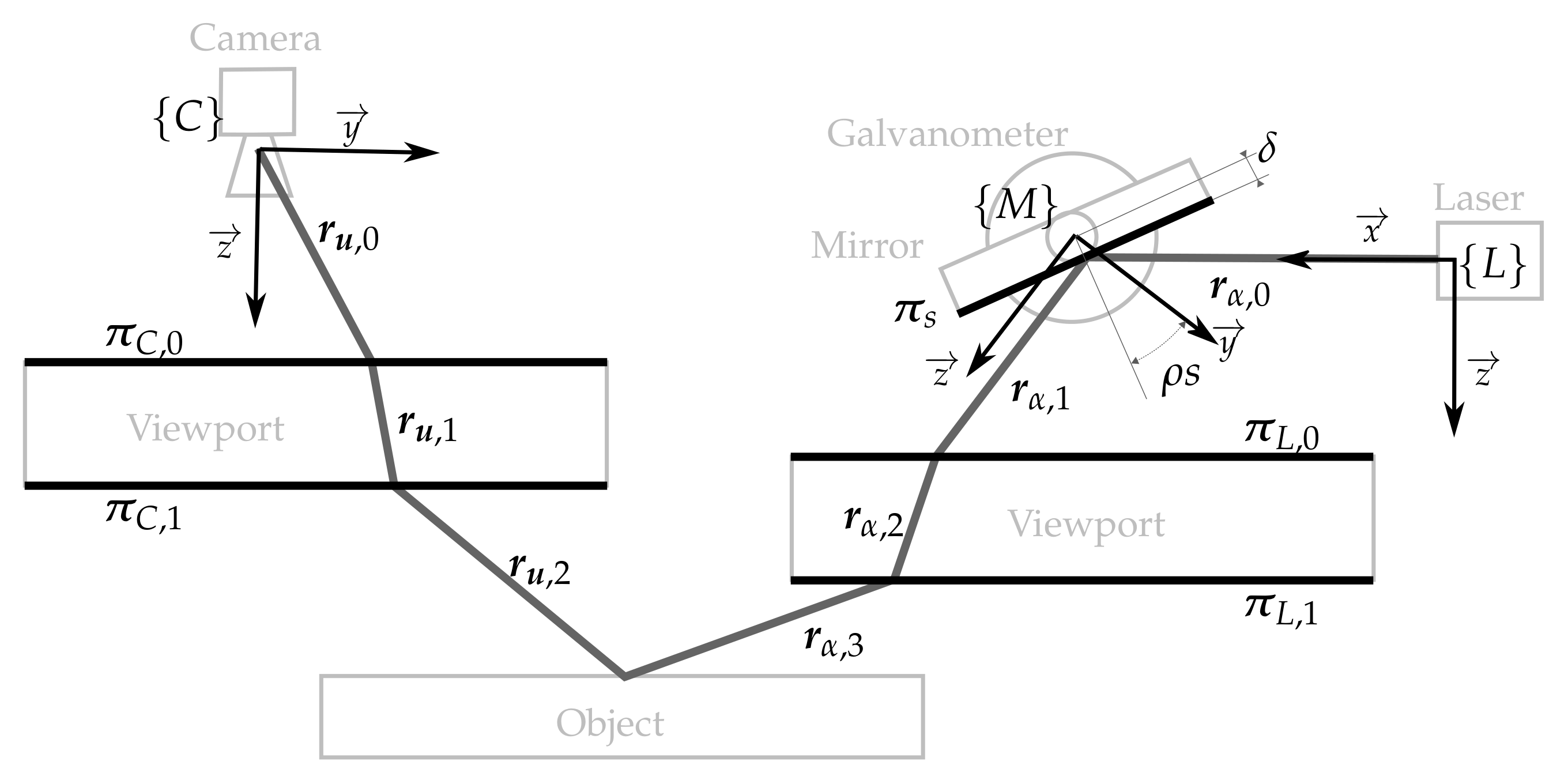
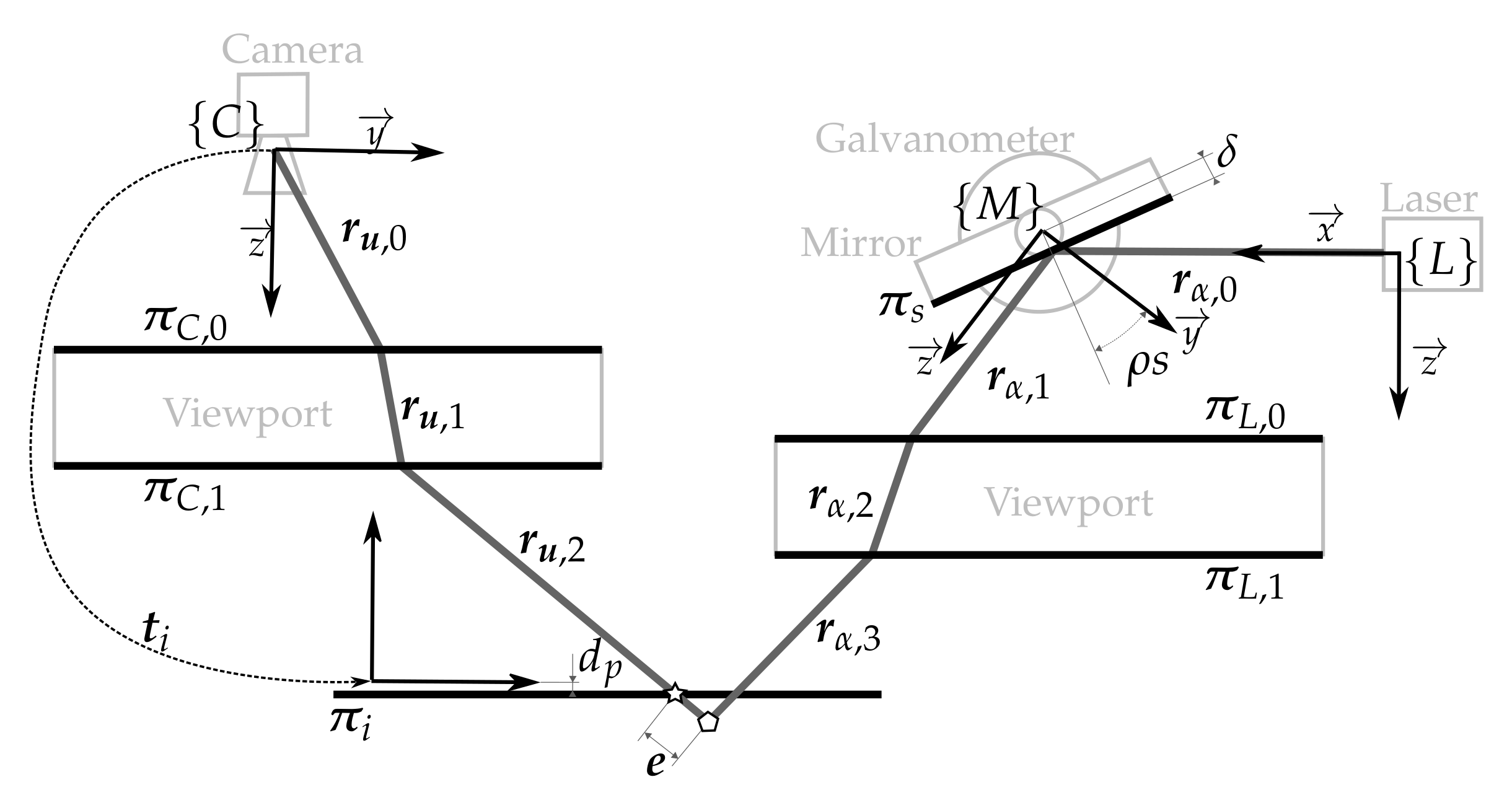
4.1. Laser Scanner Calibration
4.1.1. In-Air Camera Calibration
4.1.2. In-Air Laser Calibration
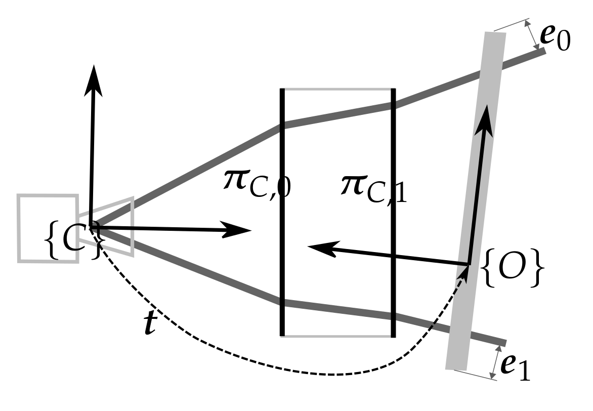
4.1.3. Camera Viewport
4.1.4. Laser Viewport
4.1.5. Elliptical Cone Fitting
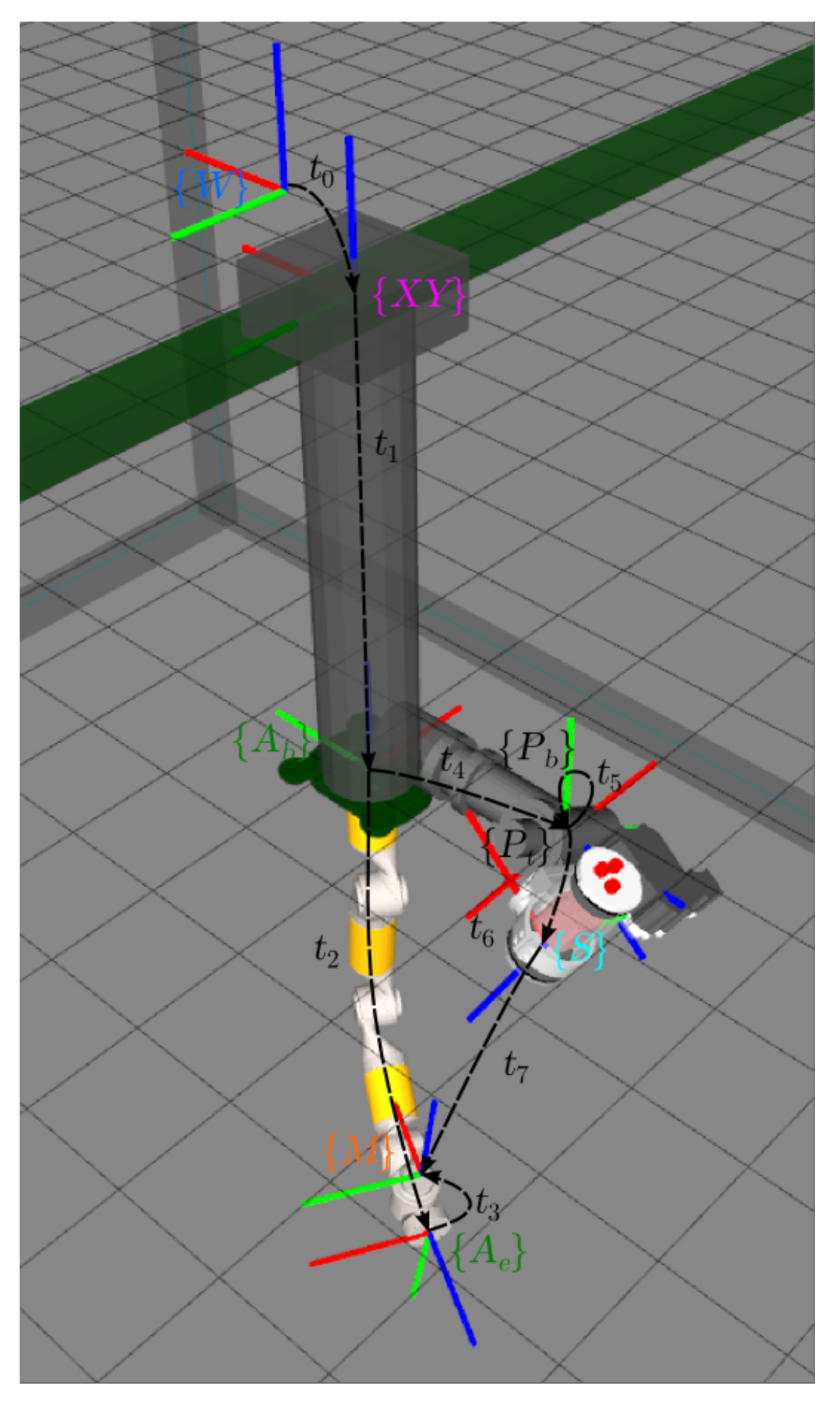
4.2. Laser Scanner-Arm Calibration
5. Experiments and Results
5.1. Sensor Accuracy
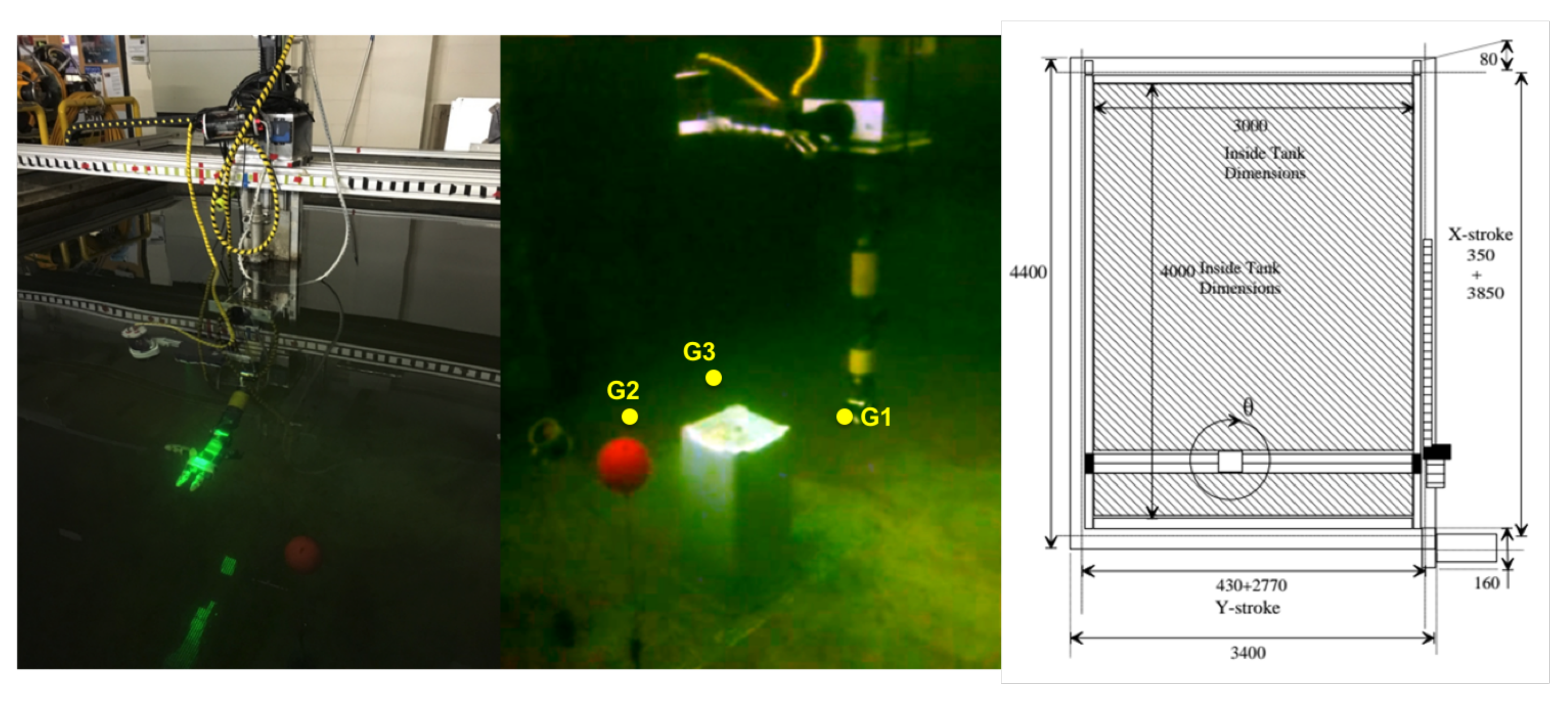
5.2. Motion Planning of a Fixed-Base Manipulator in the Presence of Unknown Fixed Obstacles
5.3. Object Grasping with a UVMS
6. Conclusions and Future Work
Supplementary Materials
Acknowledgments
Author Contributions
Conflicts of Interest
References
- Hinterstoisser, S.; Cagniart, C.; Ilic, S.; Sturm, P.; Navab, N.; Fua, P.; Lepetit, V. Gradient response maps for real-time detection of textureless objects. IEEE Trans. Pattern Anal. Mach. Intell. 2012, 34, 876–888. [Google Scholar] [CrossRef] [PubMed]
- Willow Garage, R.C. ORK: Object Recognition Kitchen. Available online: https://github.com/wg-perception/object_recognition_core (accessed on 3 April 2018).
- Wang, H.H.; Rock, S.M.; Lees, M.J. Experiments in automatic retrieval of underwater objects with an AUV. In Proceedings of the Conference MTS/IEEE Challenges of Our Changing Global Environment (OCEANS’95), San Diego, CA, USA, 9–12 October 1995; Volume 1, pp. 366–373. [Google Scholar]
- Choi, S.; Takashige, G.; Yuh, J. Experimental study on an underwater robotic vehicle: ODIN. In Proceedings of the 1994 Symposium Autonomous Underwater Vehicle Technology (AUV’94), Cambridge, MA, USA, 19–20 July 1994; pp. 79–84. [Google Scholar]
- Rigaud, V.; Coste-Maniere, E.; Aldon, M.; Probert, P.; Perrier, M.; Rives, P.; Simon, D.; Lang, D.; Kiener, J.; Casal, A.; et al. UNION: Underwater intelligent operation and navigation. IEEE Robot. Autom. Mag. 1998, 5, 25–35. [Google Scholar] [CrossRef]
- Lane, D.; O’Brien, D.J.; Pickett, M.; Davies, J.; Robinson, G.; Jones, D.; Scott, E.; Casalino, G.; Bartolini, G.; Cannata, G.; et al. AMADEUS-Advanced Manipulation for Deep Underwater Sampling. IEEE Robot. Autom. Mag. 1997, 4, 34–45. [Google Scholar] [CrossRef]
- Evans, J.; Redmond, P.; Plakas, C.; Hamilton, K.; Lane, D. Autonomous docking for Intervention-AUVs using sonar and video-based real-time 3D pose estimation. In Proceedings of the OCEANS 2003, San Diego, CA, USA, 22–26 September 2003; Volume 4, pp. 2201–2210. [Google Scholar]
- Marani, G.; Choi, S.; Yuh, J. Underwater Autonomous Manipulation for Intervention Missions AUVs. Ocean Eng. Spec. Issue AUV 2009, 36, 15–23. [Google Scholar] [CrossRef]
- Prats, M.; García, J.; Fernandez, J.; Marín, R.; Sanz, P. Advances in the specification and execution of underwater autonomous manipulation tasks. In Proceedings of the IEEE Oceans 2011, Santander, Spain, 6–9 June 2011; pp. 10361–10366. [Google Scholar]
- Prats, M.; García, J.; Wirth, S.; Ribas, D.; Sanz, P.; Ridao, P.; Gracias, N.; Oliver, G. Multipurpose autonomous underwater intervention: A systems integration perspective. In Proceedings of the 2012 20th Mediterranean Conference on Control & Automation (MED), Barcelona, Spain, 3–6 July 2012; pp. 1379–1384. [Google Scholar]
- Sanz, P.; Marín, R.; Sales, J.; Oliver, G.; Ridao, P. Recent Advances in Underwater Robotics for Intervention Missions. Soller Harbor Experiments; Low Cost Books; Psylicom Ediciones: València, Spain, 2012. [Google Scholar]
- Palomeras, N.; Penalver, A.; Massot-Campos, M.; Vallicrosa, G.; Negre, P.; Fernandez, J.; Ridao, P.; Sanz, P.; Oliver-Codina, G.; Palomer, A. I-AUV docking and intervention in a subsea panel. In Proceedings of the 2014 IEEE/RSJ International Conference on Intelligent Robots and Systems (IROS 2014), Chicago, IL, USA, 14–18 September 2014; pp. 2279–2285. [Google Scholar]
- Vallicrosa, G.; Ridao, P.; Ribas, D.; Palomer, A. Active Range-Only beacon localization for AUV homing. In Proceedings of the 2014 IEEE/RSJ International Conference on Intelligent Robots and Systems (IROS 2014), Chicago, IL, USA, 14–18 September 2014; pp. 2286–2291. [Google Scholar]
- Carrera, A.; Palomeras, N.; Ribas, D.; Kormushev, P.; Carreras, M. An Intervention-AUV learns how to perform an underwater valve turning. In Proceedings of the OCEANS 2014-TAIPEI, Taipei, Taiwan, 7–10 April 2014; pp. 1–7. [Google Scholar]
- Cieslak, P.; Ridao, P.; Giergiel, M. Autonomous underwater panel operation by GIRONA500 UVMS: A practical approach to autonomous underwater manipulation. In Proceedings of the 2015 IEEE International Conference on Robotics and Automation (ICRA), Seattle, WA, USA, 26–30 May 2015; pp. 529–536. [Google Scholar]
- Digumarti, S.T.; Chaurasia, G.; Taneja, A.; Siegwart, R.; Thomas, A.; Beardsley, P. Underwater 3D capture using a low-cost commercial depth camera. In Proceedings of the 2016 IEEE Winter Conference on Applications of Computer Vision (WACV), Lake Placid, NY, USA, 7–10 March 2016; Volume 1. [Google Scholar]
- Palomer, A.; Ridao, P.; Ribas, D.; Forest, J. Underwater 3D laser scanners: The deformation of the plane. In Lecture Notes in Control and Information Sciences; Fossen, T.I., Pettersen, K.Y., Nijmeijer, H., Eds.; Springer: Berlin, Germany, 2017; Volume 474, pp. 73–88. [Google Scholar]
- Ribas, D.; Palomeras, N.; Ridao, P.; Carreras, M.; Mallios, A. Girona 500 AUV: From Survey to Intervention. IEEE/ASME Trans. Mech. 2012, 17, 46–53. [Google Scholar] [CrossRef]
- Palomer, A.; Ridao, P.; Forest, J.; Ribas, D. Underwater Laser Scanner: Ray-based Model and Calibration. IEEE/ASME Trans. Mech. 2018. under review. [Google Scholar]
- Heikkila, J.; Silven, O. A four-step camera calibration procedure with implicit image correction. In Proceedings of the IEEE Computer Society Conference on Computer Vision and Pattern Recognition, Washington, DC, USA, 17–19 June 1997; pp. 1106–1112. [Google Scholar]
- Bradski, G. The OpenCV Library. Dobbs J. Softw. Tools 2000, 25, 120–125. [Google Scholar]
- Garrido-Jurado, S.; Muñoz-Salinas, R.; Madrid-Cuevas, F.; Marín-Jiménez, M. Automatic generation and detection of highly reliable fiducial markers under occlusion. Pattern Recognit. 2014, 47, 2280–2292. [Google Scholar] [CrossRef]
- Sucan, I.A.; Sachin, C. MoveIt! 2013. Available online: http://moveit.ros.org (accessed on 3 April 2018).
- Şucan, I.A.; Moll, M.; Kavraki, L.; Sucan, I.; Moll, M.; Kavraki, E. The open motion planning library. IEEE Robot. Autom. Mag. 2012, 19, 72–82. [Google Scholar] [CrossRef]
- Pan, J.; Chitta, S.; Manocha, D. FCL: A general purpose library for collision and proximity queries. In Proceedings of the IEEE International Conference on Robotics and Automation, Saint Paul, MN, USA, 14–18 May 2012; pp. 3859–3866. [Google Scholar]
- Hornung, A.; Wurm, K.M.; Bennewitz, M.; Stachniss, C.; Burgard, W. OctoMap: An Efficient Probabilistic 3D Mapping Framework Based on Octrees. Auton. Robots 2013, 34, 189–206. [Google Scholar] [CrossRef]
- Kuffner, J.; LaValle, S. RRT-connect: An efficient approach to single-query path planning. In Proceedings of the 2000 Millennium Conference IEEE International Conference on Robotics and Automation (ICRA), San Francisco, CA, USA, 24–28 April 2000; Volume 2, pp. 995–1001. [Google Scholar]
- Youakim, D.; Ridao, P.; Palomeras, N.; Spadafora, F.; Ribas, D.; Muzzupappa, M. MoveIt!: Autonomous Underwater Free-Floating Manipulation. IEEE Robot. Autom. Mag. 2017, 24, 41–51. [Google Scholar] [CrossRef]
- Peñalver, A.; Fernández, J.J.; Sanz, P.J. Autonomous Underwater Grasping using Multi-View Laser Reconstruction. In Proceedings of the IEEE OCEANS, Aberdeen, UK, 19–22 June 2017. [Google Scholar]
- Sanz, P.J.; Peñalver, A.; Sales, J.; Fernández, J.J.; Pérez, J.; Fornas, D.; García, J.C.; Marín, R. Multipurpose Underwater Manipulation for Archaeological Intervention. In Proceedings of the Sixth International Workshop on Marine Technology MARTECH, Cartagena, Spain, 15–17 September 2015; pp. 96–99. [Google Scholar]


© 2018 by the authors. Licensee MDPI, Basel, Switzerland. This article is an open access article distributed under the terms and conditions of the Creative Commons Attribution (CC BY) license (http://creativecommons.org/licenses/by/4.0/).
Share and Cite
Palomer, A.; Ridao, P.; Youakim, D.; Ribas, D.; Forest, J.; Petillot, Y. 3D Laser Scanner for Underwater Manipulation. Sensors 2018, 18, 1086. https://doi.org/10.3390/s18041086
Palomer A, Ridao P, Youakim D, Ribas D, Forest J, Petillot Y. 3D Laser Scanner for Underwater Manipulation. Sensors. 2018; 18(4):1086. https://doi.org/10.3390/s18041086
Chicago/Turabian StylePalomer, Albert, Pere Ridao, Dina Youakim, David Ribas, Josep Forest, and Yvan Petillot. 2018. "3D Laser Scanner for Underwater Manipulation" Sensors 18, no. 4: 1086. https://doi.org/10.3390/s18041086
APA StylePalomer, A., Ridao, P., Youakim, D., Ribas, D., Forest, J., & Petillot, Y. (2018). 3D Laser Scanner for Underwater Manipulation. Sensors, 18(4), 1086. https://doi.org/10.3390/s18041086