Sensor-Based Optimized Control of the Full Load Instability in Large Hydraulic Turbines


Abstract
1. Introduction
2. Full Load Instability in the Francis Turbine and Experimental Set-Up
2.1. General Description of the Unit and the Phenomena
2.2. Sensors Installed and Acquisition Strategy
3. Signal Analysis
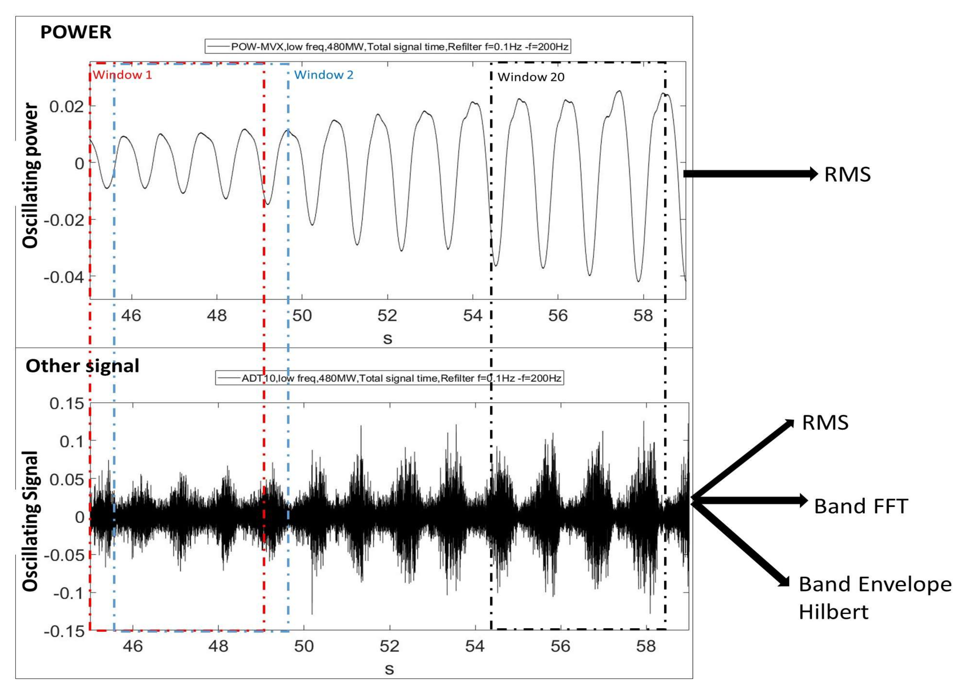
3.1. RMS Values
3.2. FFT Analysis
3.3. Envelope Characteristic Frequencies with Hilbert Transform
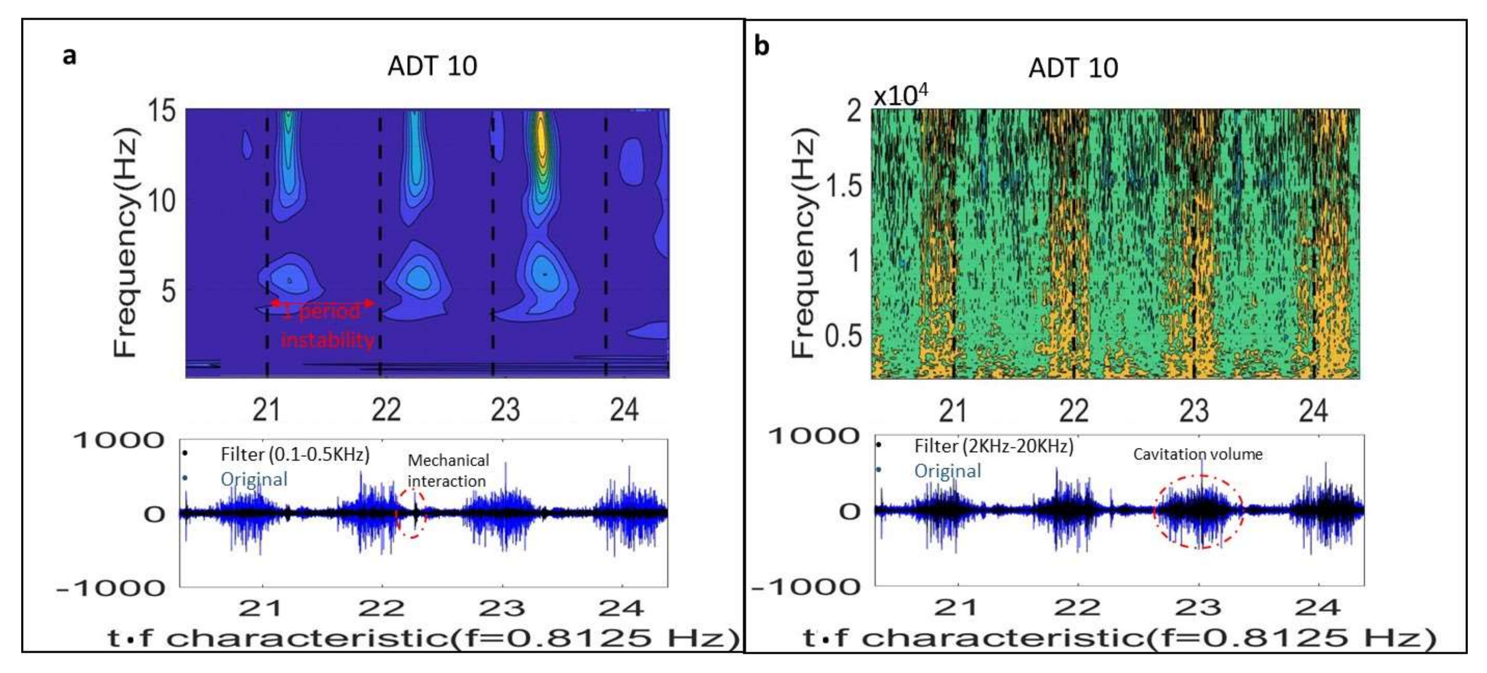
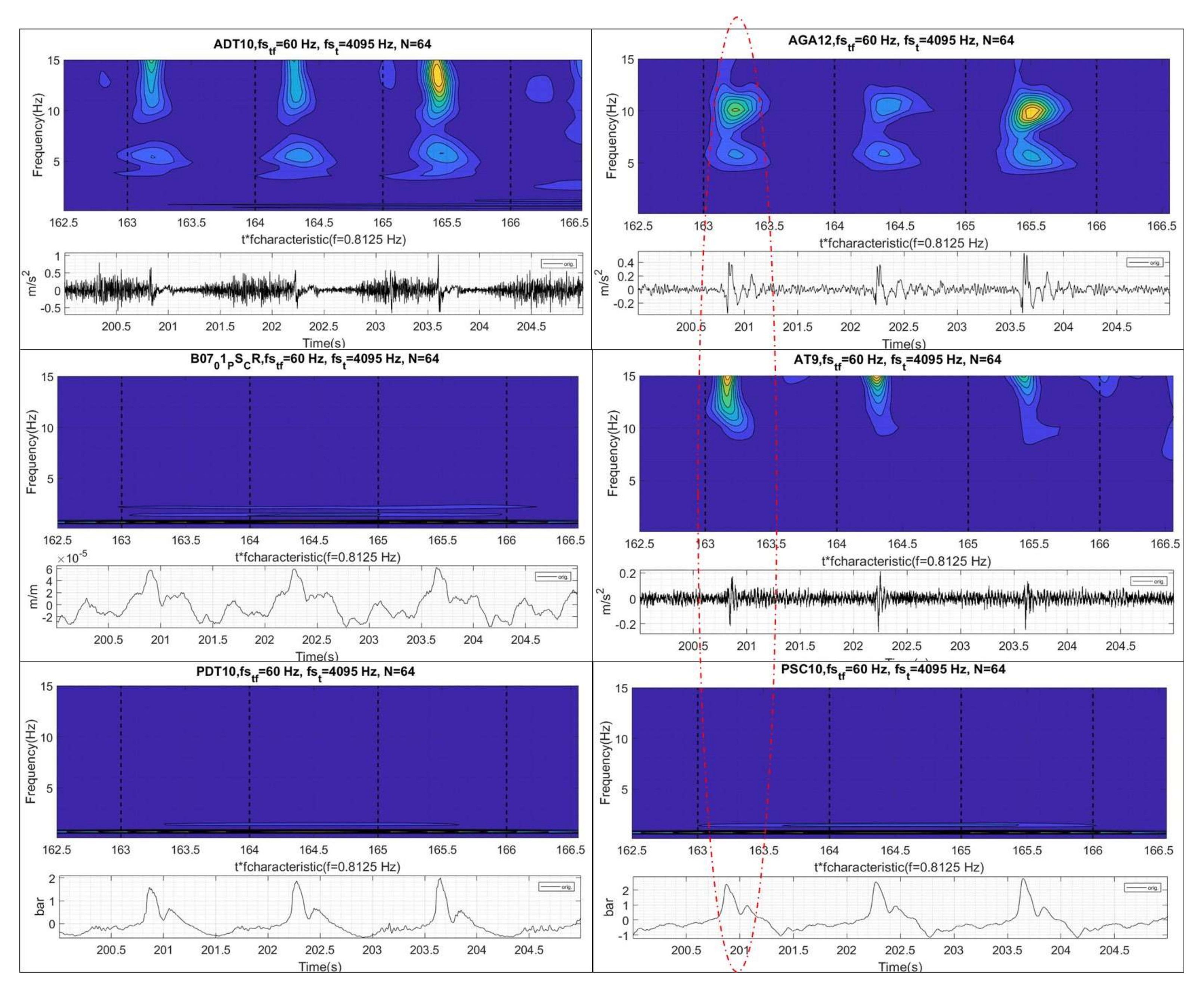
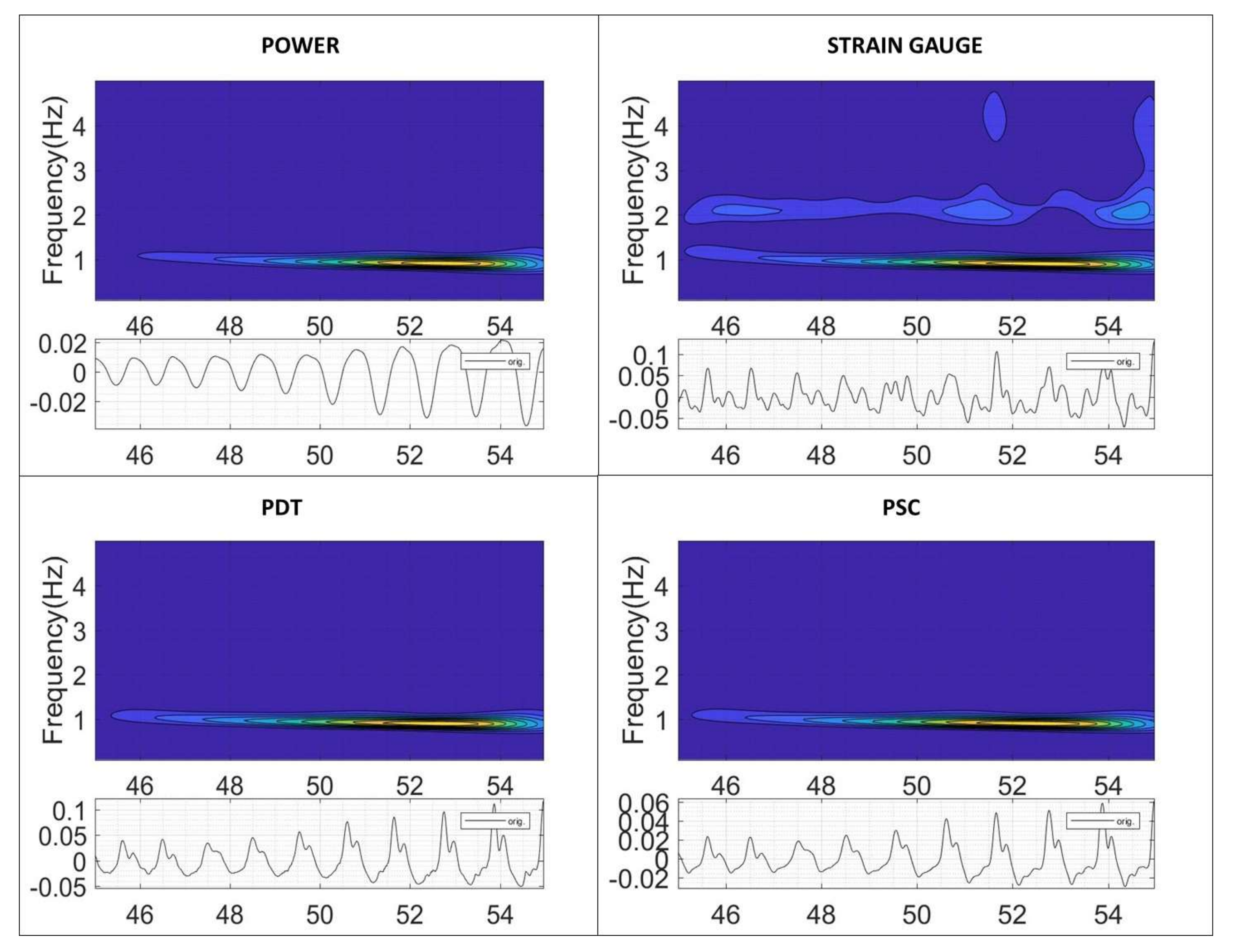
3.4. Time-Frequency Analysis with Wavelet
4. Results and Analysis of an Optimized Acquisition Strategy
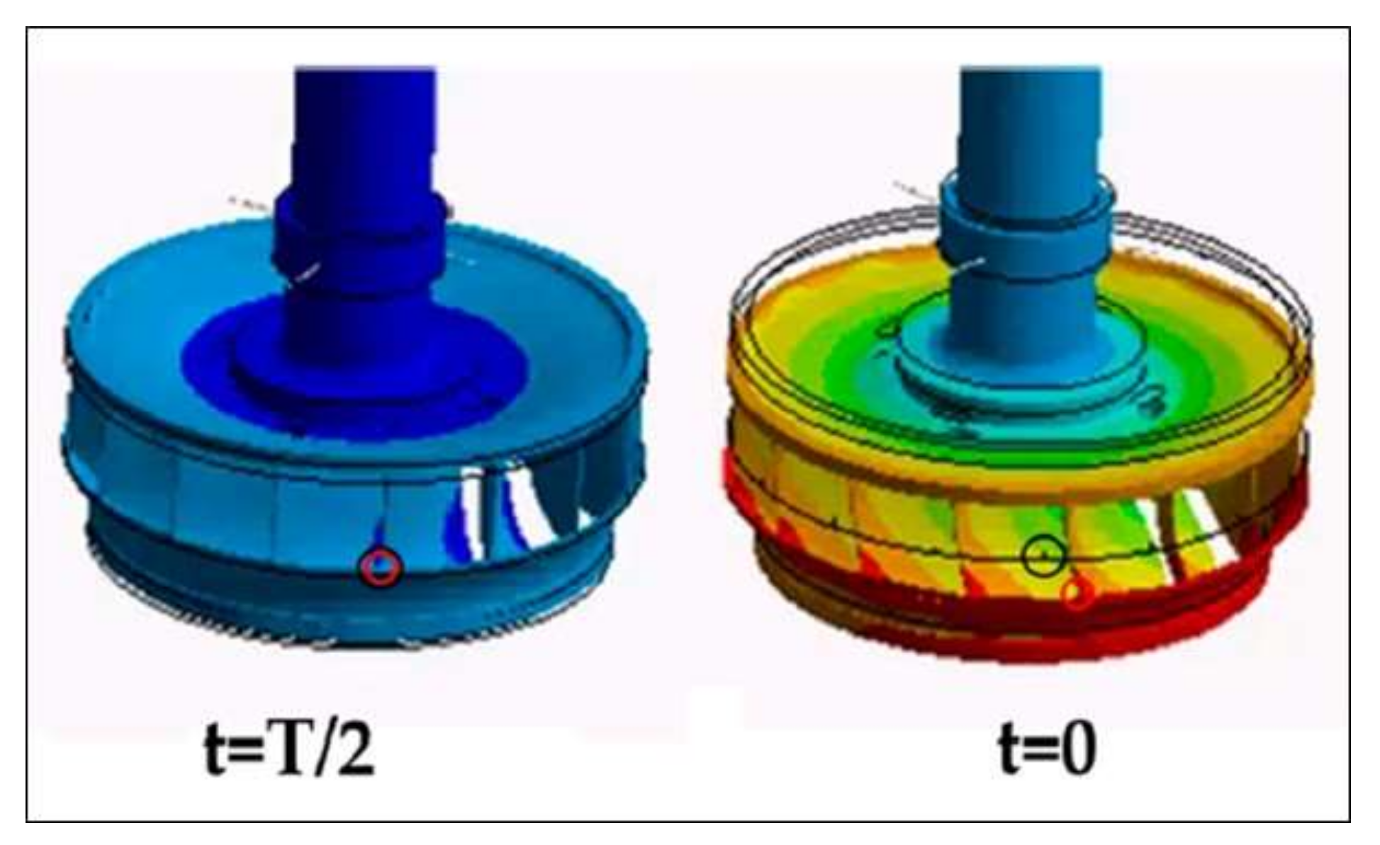
4.1. Analysis of the Instability: Comparison with the Reduced Scale Model
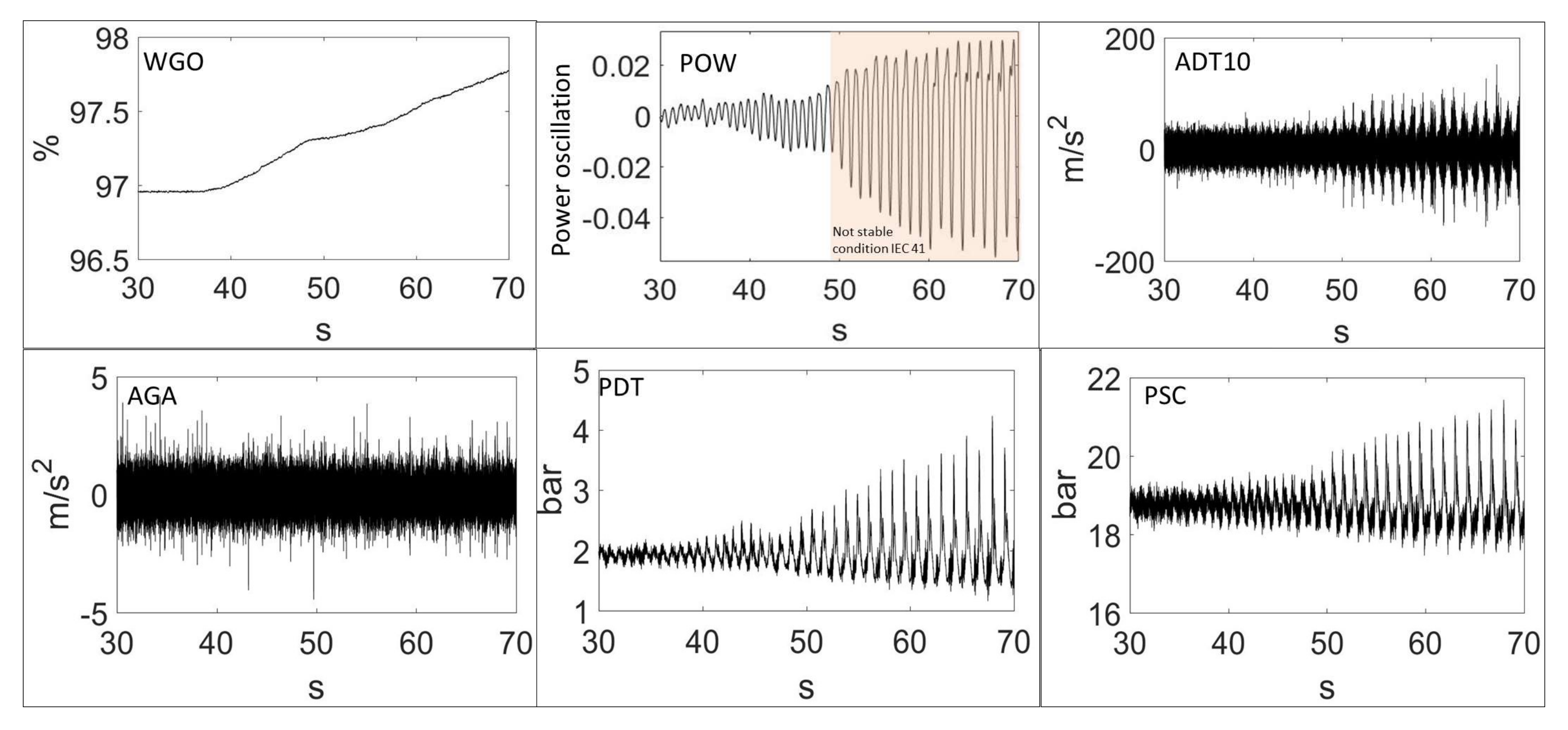
4.2. Time and Time-Frequency Characteristic of the Instability Onset
4.3. Sensitivity to the Detect the Instability Onset
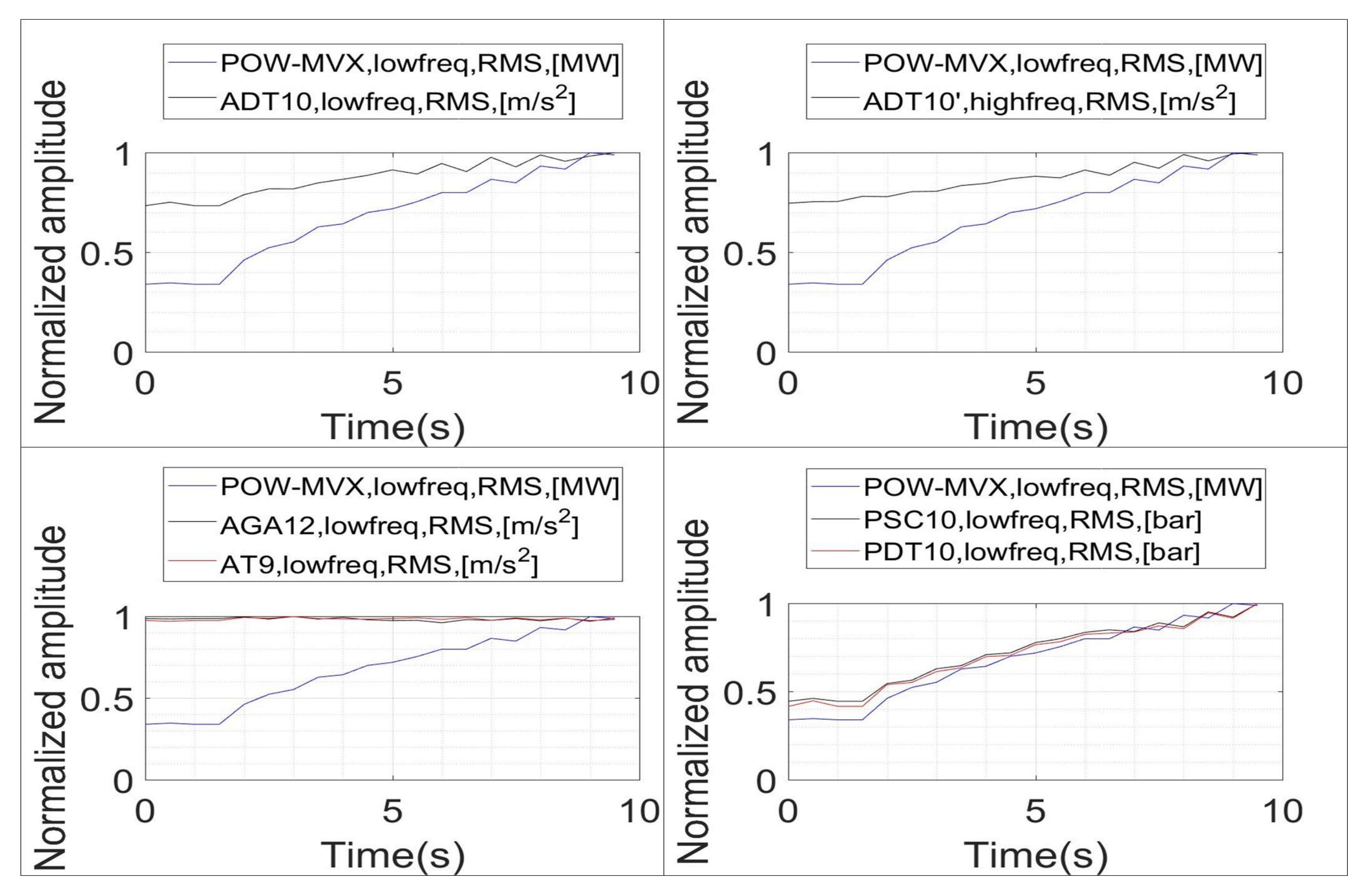
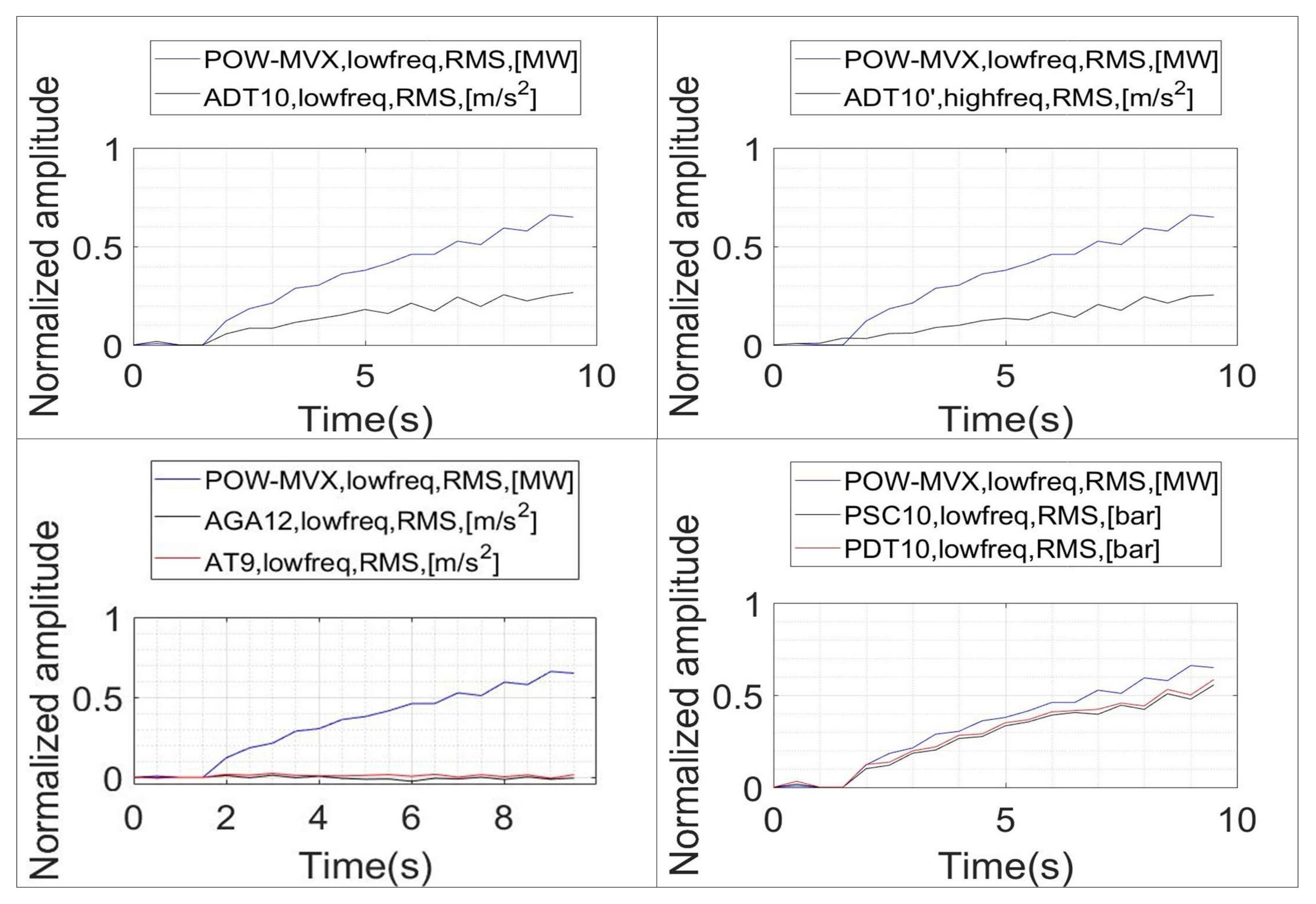
4.3.1. RMS Indicators
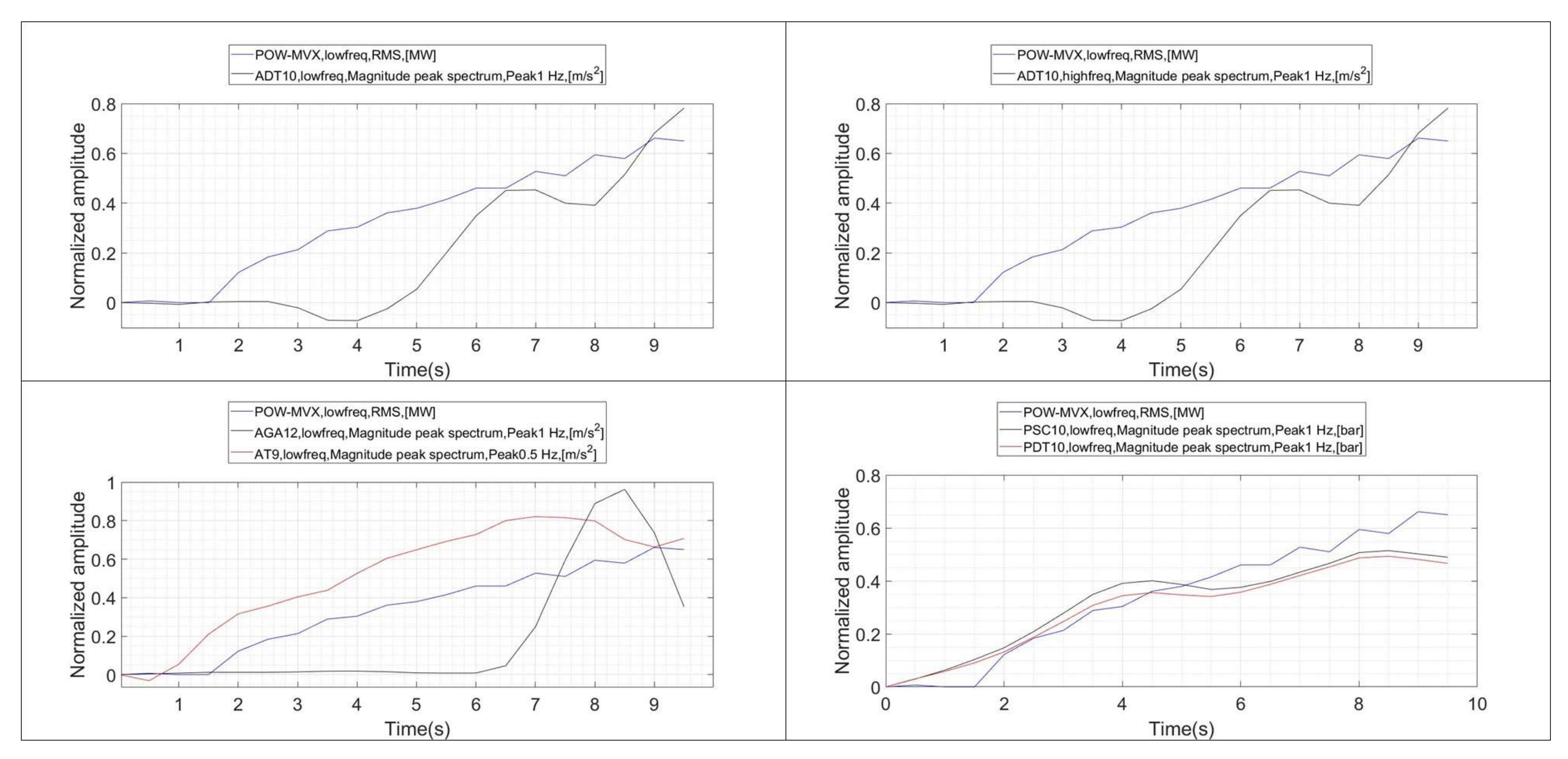
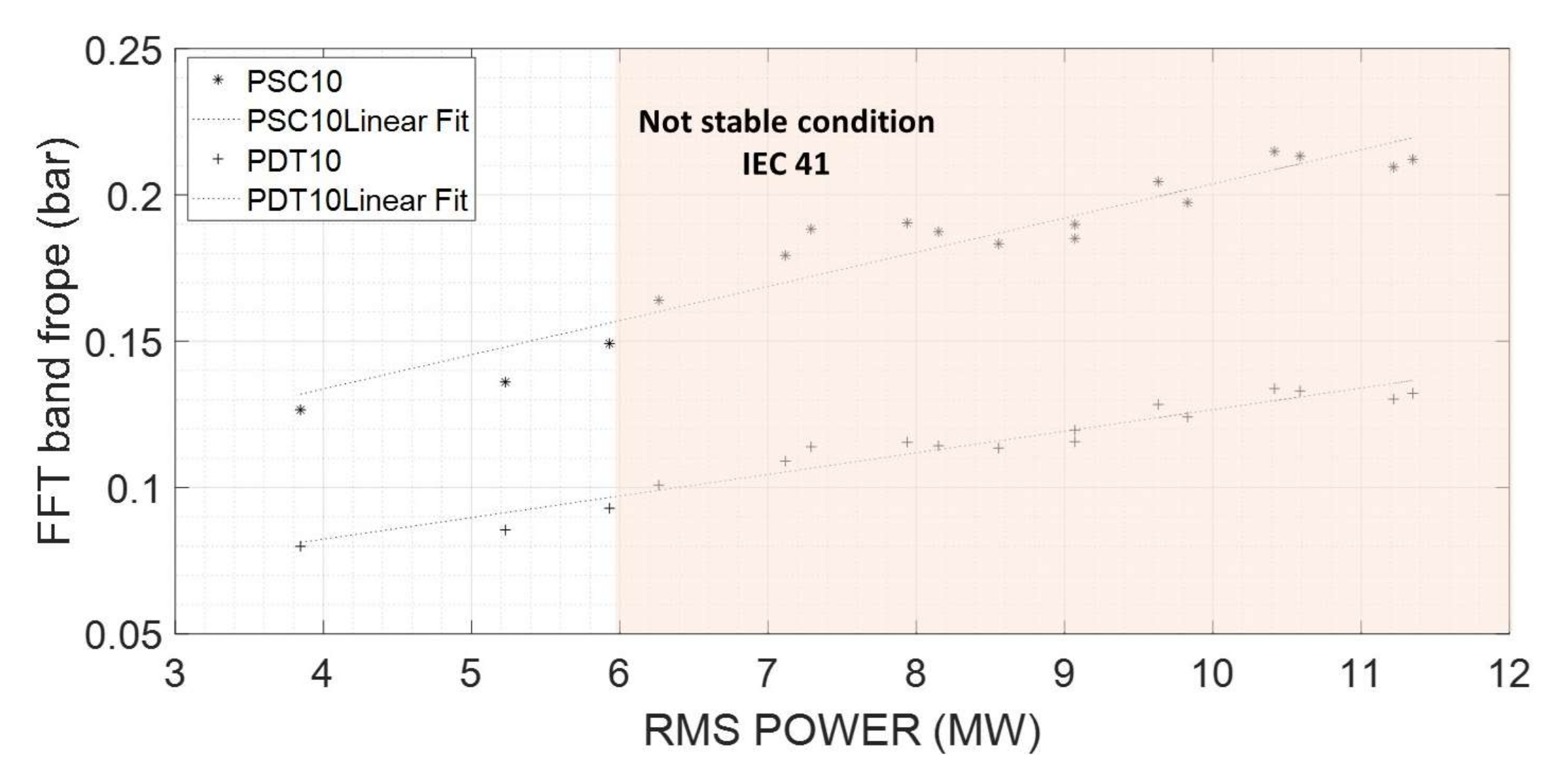
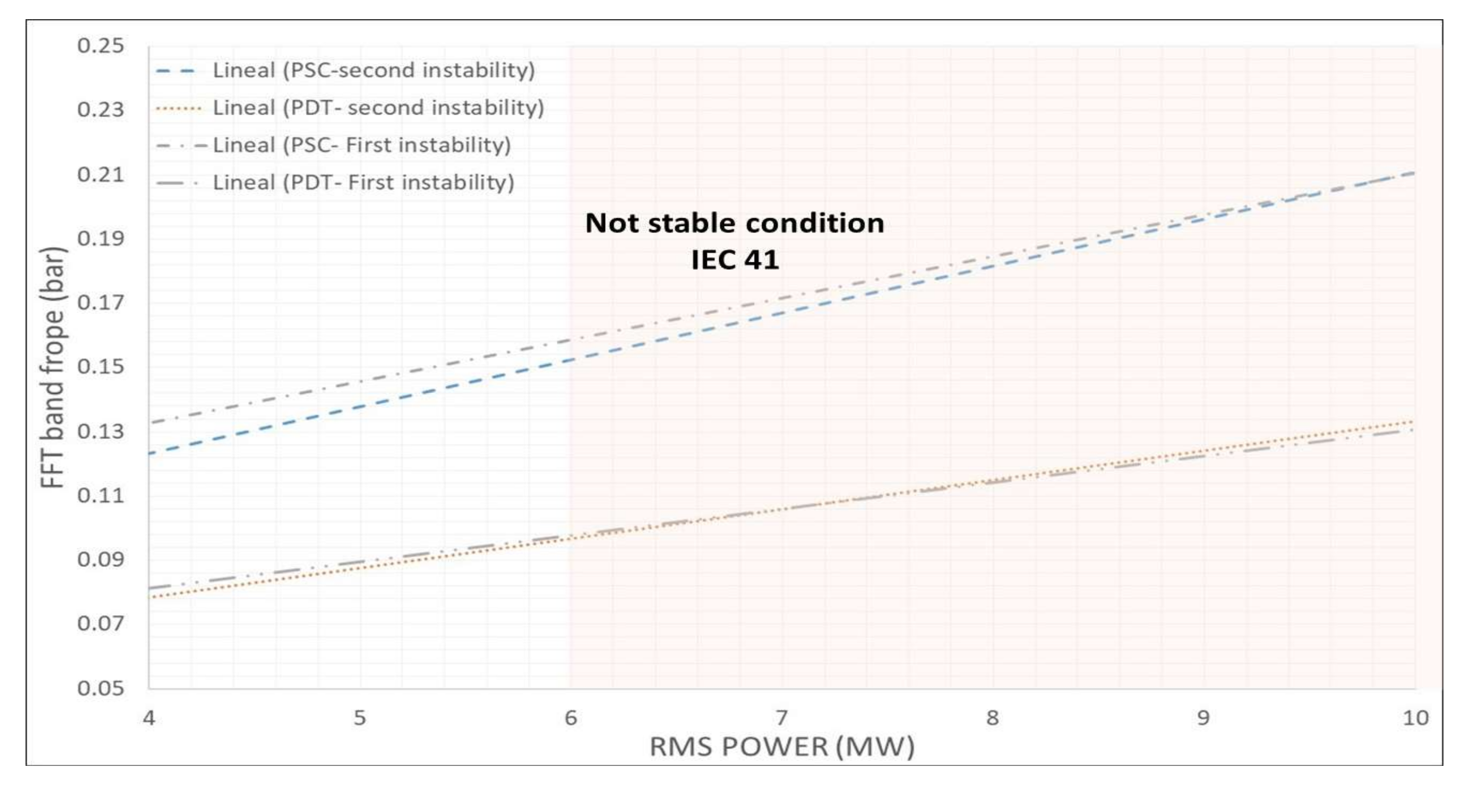
4.3.2. FFT Band
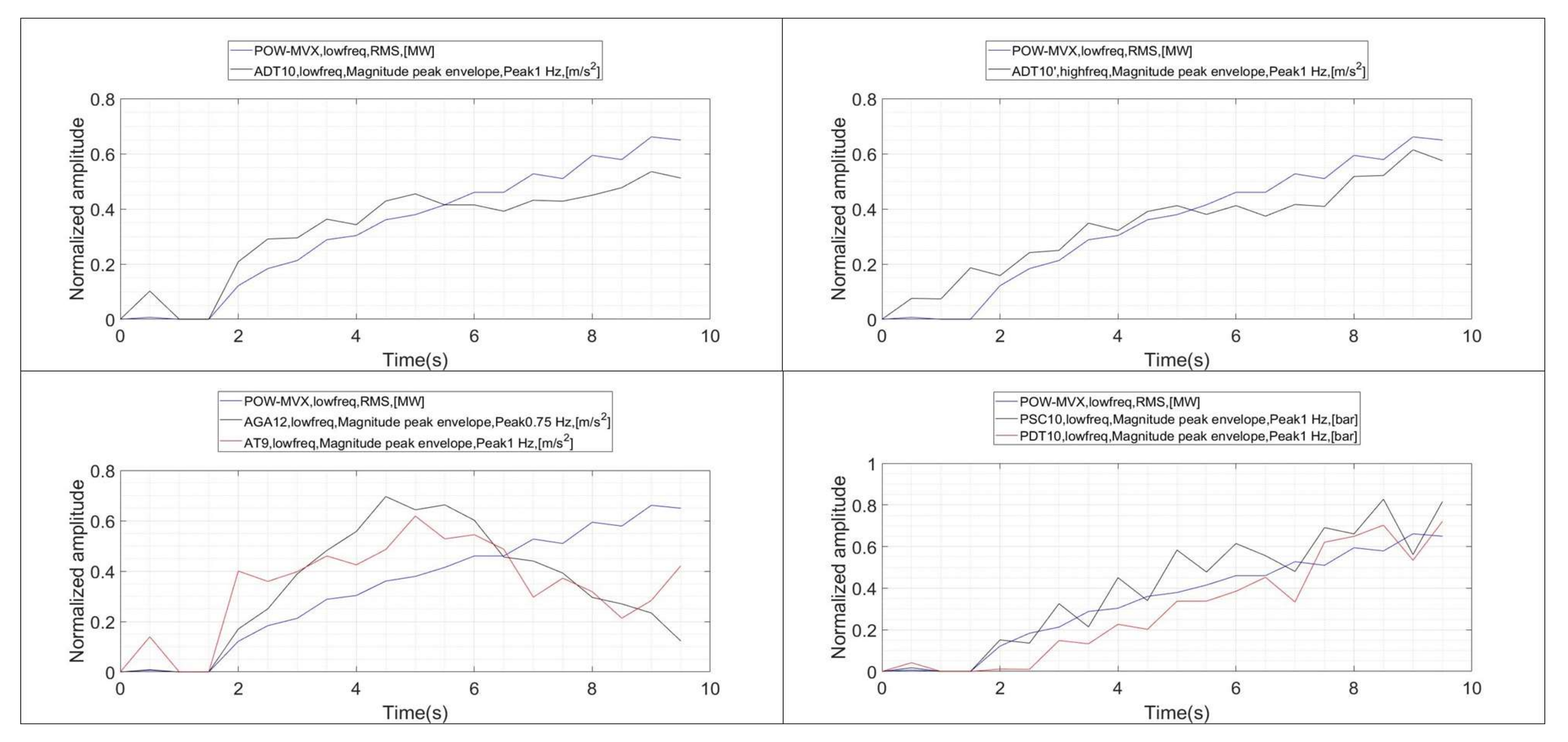
4.3.3. Envelope through Hilbert Transform
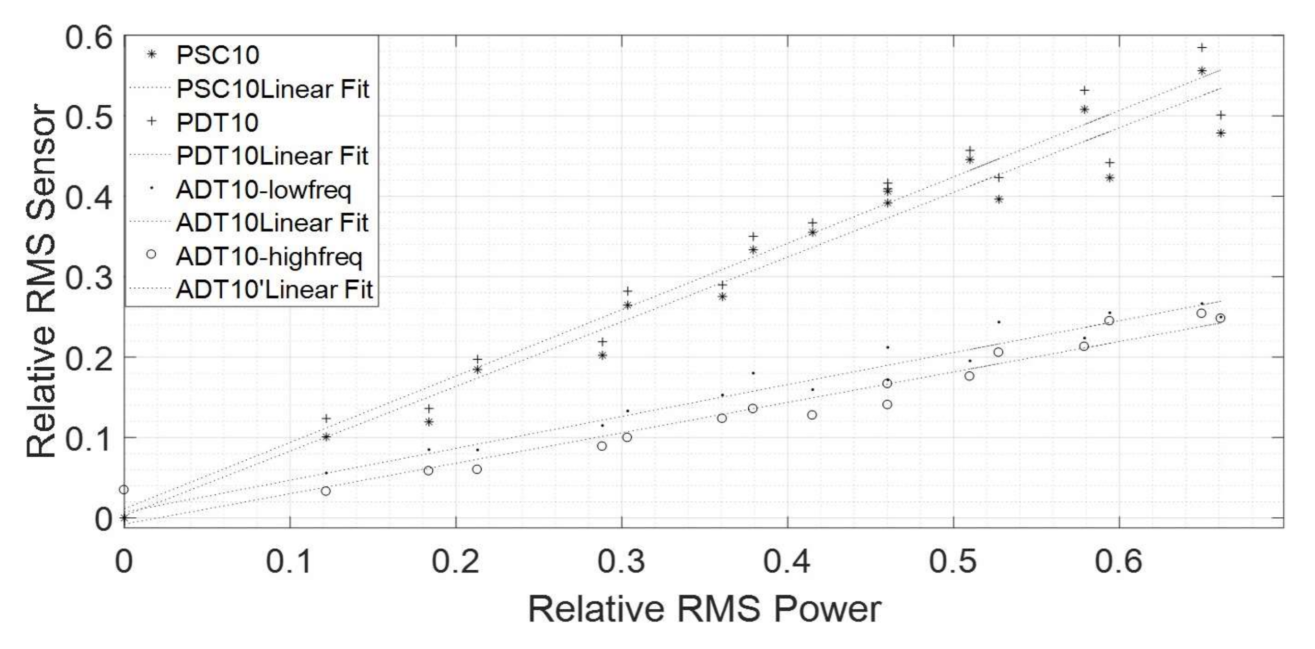
4.3.4. Linear Regression and Optimization
- Linearity with respect to : It is desirable that the indicators follow a linear correlation with the in order to simplify the control model of the instability and in order to predict the oscillating power (Figure 15).
- Slope of the correlation vs. Indicator: Higher slopes will indicate a more sensitive indicator to detect a variation in the RMS of the oscillating power.
- Advancement with respect increasing power: If the two preceding indicators are achieved a third indicator is the advancement, which helps to advance the detection of the instability (reactivity). Graphically it can be seen as the value of the indicator, when starts to increase (approximately at t = 1.5 s in Figure 12, Figure 13 and Figure 14).
- of the pressure sensors,
- for the pressure sensors,
- for ADT-highfreq.
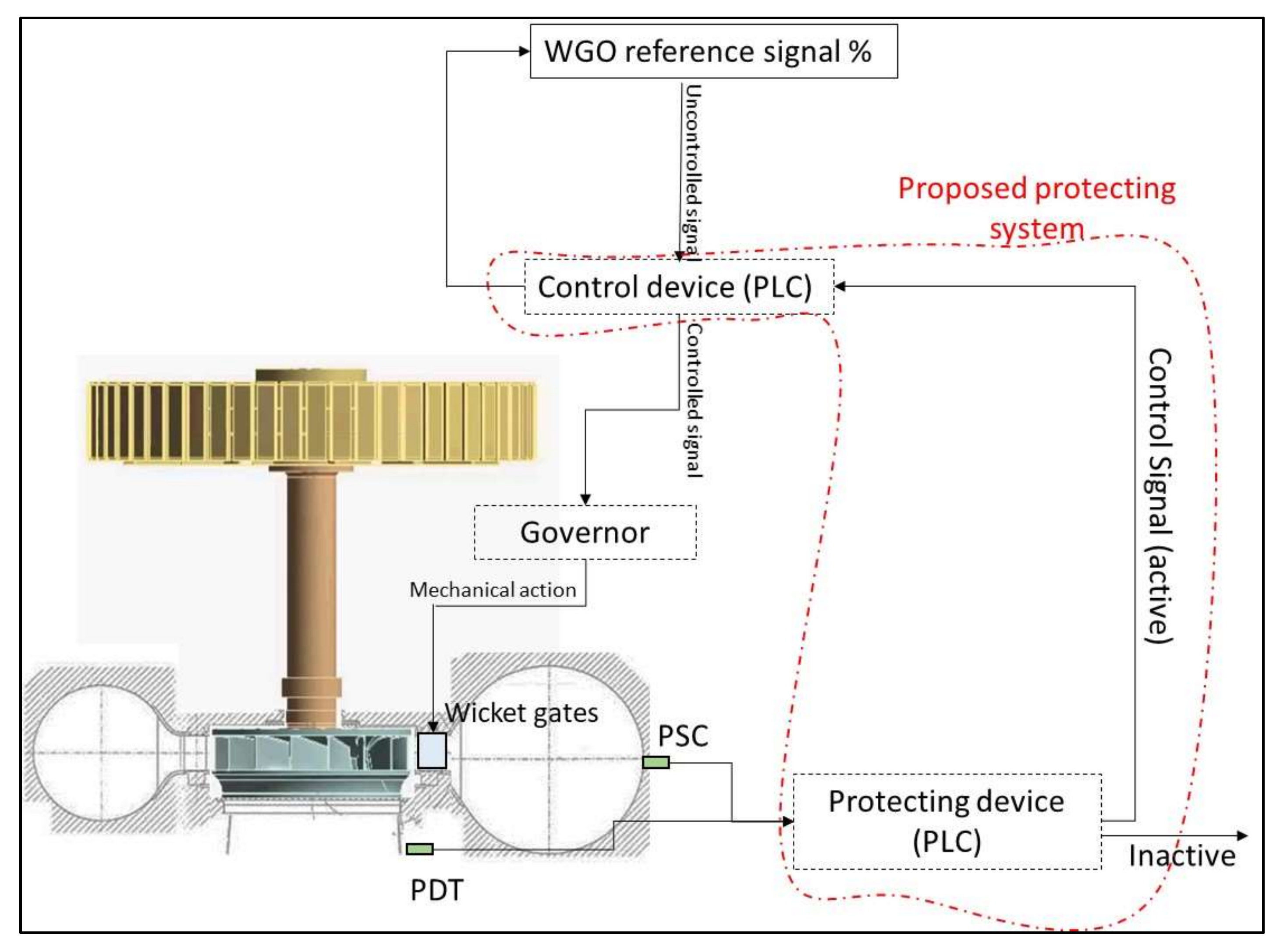
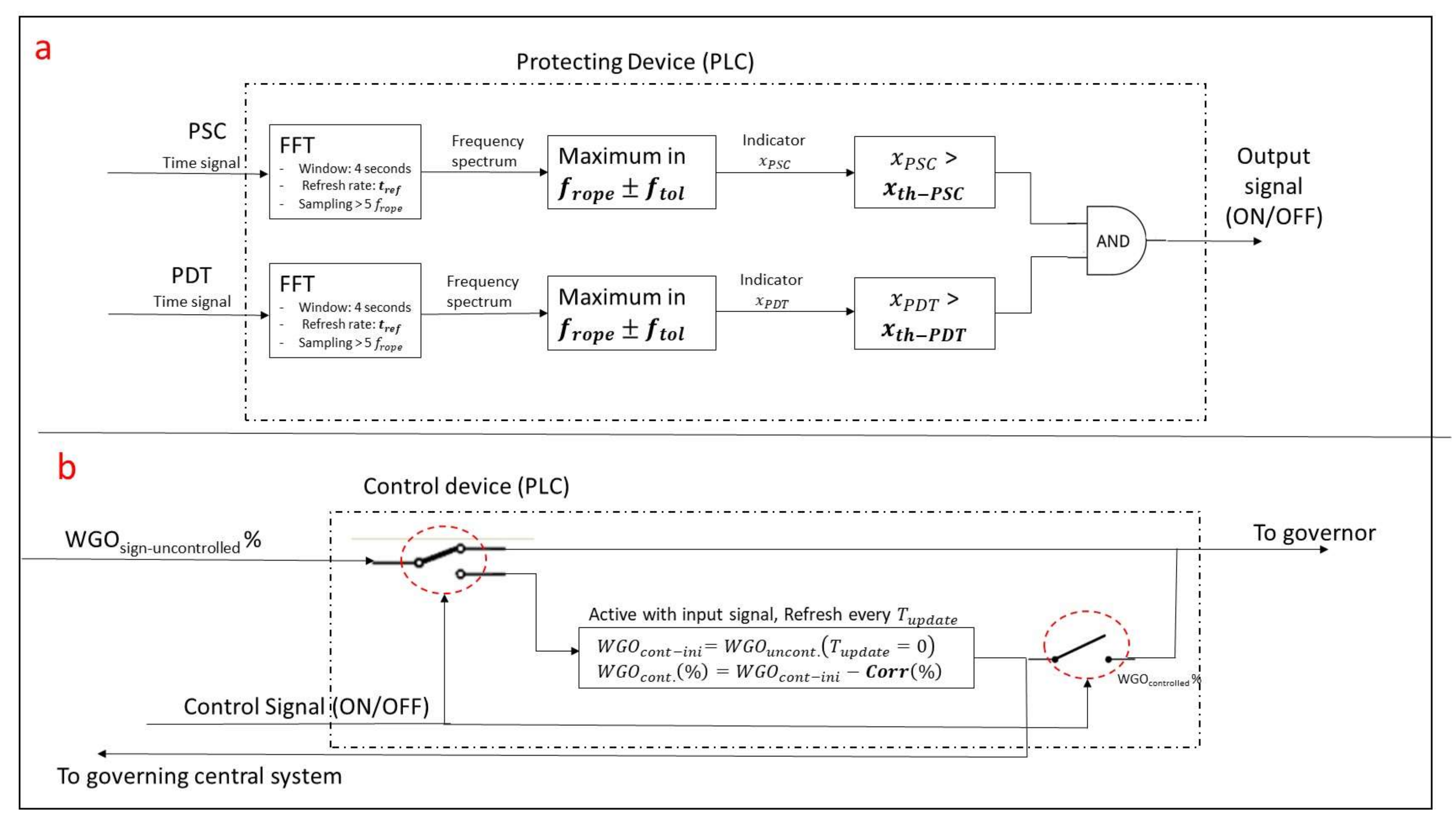
5. Proposed Protection System to Increase the Operating Range of the Unit
6. Conclusions
Acknowledgments
Author Contributions
Conflicts of Interest
References
- Valero, C.; Egusquiza, M.; Egusquiza, E.; Presas, A.; Valentin, D.; Bossio, M. Extension of Operating Range in Pump-Turbines. Influence of Head and Load. Energies 2017, 10, 2178. [Google Scholar] [CrossRef]
- De Siervo, F.; De Leva, F. Modern trends in selecting and designing Francis turbines. Water Power Dam Constr. 1976, 28, 28–35. [Google Scholar]
- Escaler, X.; Egusquiza, E.; Farhat, M.; Avellan, F.; Coussirat, M. Detection of cavitation in hydraulic turbines. Mech. Syst. Signal Process. 2006, 20, 983–1007. [Google Scholar] [CrossRef]
- Kumar, P.; Saini, R.P. Study of cavitation in hydro turbines—A review. Renew. Sustain. Energy Rev. 2010, 14, 374–383. [Google Scholar] [CrossRef]
- Luo, X.-W.; Ji, B.; Tsujimoto, Y. A review of cavitation in hydraulic machinery. J. Hydrodyn. Ser. B 2016, 28, 335–358. [Google Scholar] [CrossRef]
- Liu, X.; Luo, Y.; Wang, Z. A review on fatigue damage mechanism in hydro turbines. Renew. Sustain. Energy Rev. 2016, 54, 1–14. [Google Scholar] [CrossRef]
- Egusquiza, E.; Valero, C.; Huang, X.; Jou, E.; Guardo, A.; Rodriguez, C. Failure investigation of a large pump-turbine runner. Eng. Fail. Anal. 2012, 23, 27–34. [Google Scholar] [CrossRef]
- Gagnon, M.; Tahan, A.; Bocher, P.; Thibault, D. On the fatigue reliability of hydroelectric Francis runners. Procedia Eng. 2013, 66, 565–574. [Google Scholar] [CrossRef][Green Version]
- Egusquiza, E.; Valero, C.; Estévez, A.; Guardo, A.; Coussirat, M. Failures due to ingested bodies in hydraulic turbines. Eng. Fail. Anal. 2011, 18, 464–473. [Google Scholar] [CrossRef]
- Egusquiza, M.; Egusquiza, E.; Valentin, D.; Valero, C.; Presas, A. Failure investigation of a Pelton turbine runner. Eng. Fail. Anal. 2017, 81, 234–244. [Google Scholar] [CrossRef]
- Rheingans, W. Power swings in hydroelectric power plants. Trans. ASME 1940, 62, 171–184. [Google Scholar]
- Valentín, D.; Presas, A.; Egusquiza, E.; Valero, C.; Egusquiza, M.; Bossio, M. Power Swing Generated in Francis Turbines by Part Load and Overload Instabilities. Energies 2017, 10, 2124. [Google Scholar] [CrossRef]
- Favrel, A.; Landry, C.; Müller, A.; Yamamoto, K.; Avellan, F. Hydro-acoustic resonance behavior in presence of a precessing vortex rope: Observation of a lock-in phenomenon at part load Francis turbine operation. IOP Conf. Ser. Earth Environ. Sci. 2014, 22, 032035. [Google Scholar] [CrossRef]
- Favrel, A.; Müller, A.; Landry, C.; Gomes, J.; Yamamoto, K.; Avellan, F. Dynamics of the precessing vortex rope and its interaction with the system at Francis turbines part load operating conditions. J. Phys. Conf. Ser. 2017, 813. [Google Scholar] [CrossRef]
- Favrel, A.; Müller, A.; Landry, C.; Yamamoto, K.; Avellan, F. Study of the vortex-induced pressure excitation source in a Francis turbine draft tube by particle image velocimetry. Exp. Fluids 2015, 56, 215. [Google Scholar] [CrossRef]
- Favrel, A.; Müller, A.; Landry, C.; Yamamoto, K.; Avellan, F. LDV survey of cavitation and resonance effect on the precessing vortex rope dynamics in the draft tube of Francis turbines. Exp. Fluids 2016, 57, 168. [Google Scholar] [CrossRef]
- Müller, A.; Favrel, A.; Landry, C.; Avellan, F. Fluid–structure interaction mechanisms leading to dangerous power swings in Francis turbines at full load. J. Fluids Struct. 2017, 69, 56–71. [Google Scholar] [CrossRef]
- Müller, A.; Favrel, A.; Landry, C.; Yamamoto, K.; Avellan, F. On the physical mechanisms governing self-excited pressure surge in Francis turbines. IOP Conf. Ser. Earth Environ. Sci. 2014, 22. [Google Scholar] [CrossRef]
- Valero, C.; Egusquiza, E.; Presas, A.; Valentin, D.; Egusquiza, M.; Bossio, M. Condition monitoring of a prototype turbine. Description of the system and main results. J. Phys. Conf. Ser. 2017, 813, 012041. [Google Scholar] [CrossRef]
- Egusquiza, E.; Valero, C.; Valentin, D.; Presas, A.; Rodriguez, C.G. Condition monitoring of pump-turbines. New challenges. Measurement 2015, 67, 151–163. [Google Scholar] [CrossRef]
- Egusquiza, M.; Egusquiza, E.; Valero, C.; Presas, A.; Valentín, D.; Bossio, M. Advanced condition monitoring of Pelton turbines. Measurement 2018, 119, 46–55. [Google Scholar] [CrossRef]
- HYdropower Plants PERformance and flexiBle Operation towards Lean Integration of New Renewable Energies. Available online: https://hyperbole.epfl.ch (accessed on 12 December 2017).
- Valentín, D.; Presas, A.; Bossio, M.; Egusquiza, M.; Egusquiza, E.; Valero, C. Feasibility of Detecting Natural Frequencies of Hydraulic Turbines While in Operation, Using Strain Gauges. Sensors 2018, 18, 174. [Google Scholar] [CrossRef] [PubMed]
- Müller, A.; Dreyer, M.; Andreini, N.; Avellan, F. Draft tube discharge fluctuation during self-sustained pressure surge: Fluorescent particle image velocimetry in two-phase flow. Exp. Fluids 2013, 54, 1514. [Google Scholar] [CrossRef]
- Presas, A.; Valentin, D.; Egusquiza, E.; Valero, C. Detection and analysis of part load and full load instabilities in a real Francis turbine prototype. J. Phys. Conf. Ser. 2017, 813, 012038. [Google Scholar] [CrossRef]
- Batllo, A.P.; Valentin, D.; Egusquiza, M.; Bossio, M.; Egusquiza, E.; Valero, C. Optimized Use of Sensors to Detect Critical Full Load Instability in Large Hydraulic Turbines. Proceedings 2017, 1, 822. [Google Scholar] [CrossRef]
- Koutnik, J.; Krüger, K.; Pochyly, F.; Rudolf, P.; Haban, V. On cavitating vortex rope form stability during Francis turbine part load operation. In Proceedings of the IAHR International Meeting of the Workgroup on Cavitation and Dynamic Problems in Hydraulic Machinery and Systems, Barcelona, Spain, 28–30 June 2006. [Google Scholar]
- Ruprecht, A.; Helmrich, T.; Aschenbrenner, T.; Scherer, T. Simulation of vortex rope in a turbine draft tube. In Proceedings of the 22nd IAHR Symposium on Hydraulic Machinery and Systems, Stockholm, Sweden, 29 June–2 July 2002; pp. 9–12. [Google Scholar]
- Oppenheim, A.V. Discrete-Time Signal Processing; Pearson Education India: Chennai, India, 1999. [Google Scholar]
- Presas, A.; Valentin, D.; Egusquiza, E.; Valero, C.; Seidel, U. On the detection of natural frequencies and mode shapes of submerged rotating disk-like structures from the casing. Mech. Syst. Signal Process. 2015, 60, 547–570. [Google Scholar] [CrossRef]
- Newland, D.E. Wavelet Analysis of Vibration: Part 1—Theory. J. Vib. Acoust. 1994, 116, 409–416. [Google Scholar] [CrossRef]
- Chui, C.K. Wavelet Analysis and Its Applications; DTIC Document; Defense Technical Information Center: Fort Belvoir, VA, USA, 1995. [Google Scholar]
- Wang, Y.; He, Z.; Zi, Y. Enhancement of signal denoising and multiple fault signatures detecting in rotating machinery using dual-tree complex wavelet transform. Mech. Syst. Signal Process. 2010, 24, 119–137. [Google Scholar] [CrossRef]
- Newland, D.E. An Introduction to Random Vibrations, Spectral & Wavelet Analysis; Courier Dover Publications: Mineola, NY, USA, 2012. [Google Scholar]
- Ewins, D.J. Modal Testing Theory and Practice; Research Studies Press: Baldock, UK, 1984. [Google Scholar]


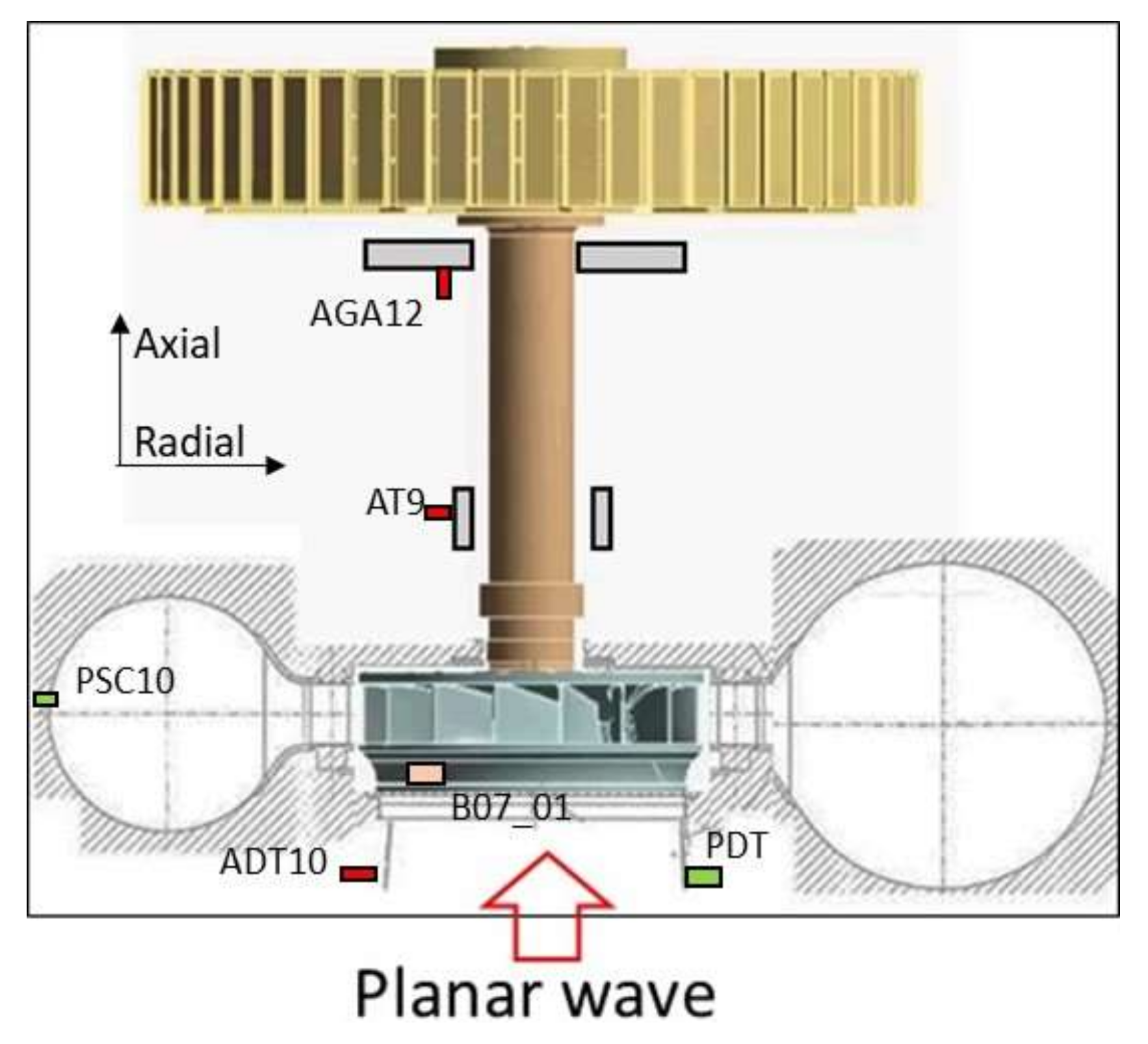
| Sensor Name | Physical Unit | Location, Direction | Sensitivity |
|---|---|---|---|
| ADT 10 | Draft tube wall Radial direction | ||
| AT 9 | Turbine guide bearing Radial direction | ||
| AGA 12 | Generator bearing Axial direction | ||
| PSC 10 | Pa | Draft tube pick-up pressure hole radial | |
| PDT 10 | Pa | Spiral casing pick-up pressure hole radial | |
| B07_01 | Runner blade trailing edge |
| Sensor | RMS | FFT | Envelope | ||||||
|---|---|---|---|---|---|---|---|---|---|
| Slope | Intercept | R2 | Slope | Intercept | R2 | Slope | Intercept | R2 | |
| ADT-low freq. | 0.39 | 0.007 | 0.96 | 1.26 | −0.26 | 0.65 | 0.61 | 0.13 | 0.83 |
| ADT-high freq. | 0.38 | −0.008 | 0.94 | 1.26 | −0.26 | 0.65 | 0.64 | 0.13 | 0.93 |
| PDT | 0.83 | 0.01 | 0.96 | 0.63 | 0.1 | 0.94 | 1.18 | −0.13 | 0.85 |
| PSC | 0.80 | 0.003 | 0.96 | 0.62 | 0.13 | 0.93 | 1.14 | 0.01 | 0.82 |
| Parameter | Present Case | Comments |
|---|---|---|
| Window length (FFT) | 4 s | Less is not recommendable (resolution in frequency) |
| Refresh rate (FFT) | 0.5 s | Enough small to have a reactive system |
| Sampling rate | 10 samples/s | >5· |
| Hz | To be determined experimentally | |
| 0.15 and 0.1 | To be determined experimentally according to IEC 41 | |
| Corr (%) | 1% | To be determined experimentally testing the exit of the instability |
| 2 | To be determined experimentally testing the exit of the instability |
© 2018 by the authors. Licensee MDPI, Basel, Switzerland. This article is an open access article distributed under the terms and conditions of the Creative Commons Attribution (CC BY) license (http://creativecommons.org/licenses/by/4.0/).
Share and Cite
Presas, A.; Valentin, D.; Egusquiza, M.; Valero, C.; Egusquiza, E. Sensor-Based Optimized Control of the Full Load Instability in Large Hydraulic Turbines. Sensors 2018, 18, 1038. https://doi.org/10.3390/s18041038
Presas A, Valentin D, Egusquiza M, Valero C, Egusquiza E. Sensor-Based Optimized Control of the Full Load Instability in Large Hydraulic Turbines. Sensors. 2018; 18(4):1038. https://doi.org/10.3390/s18041038
Chicago/Turabian StylePresas, Alexandre, David Valentin, Mònica Egusquiza, Carme Valero, and Eduard Egusquiza. 2018. "Sensor-Based Optimized Control of the Full Load Instability in Large Hydraulic Turbines" Sensors 18, no. 4: 1038. https://doi.org/10.3390/s18041038
APA StylePresas, A., Valentin, D., Egusquiza, M., Valero, C., & Egusquiza, E. (2018). Sensor-Based Optimized Control of the Full Load Instability in Large Hydraulic Turbines. Sensors, 18(4), 1038. https://doi.org/10.3390/s18041038