Reconstruction of Cylindrical Surfaces Using Digital Image Correlation


Abstract
1. Introduction
2. Methodology
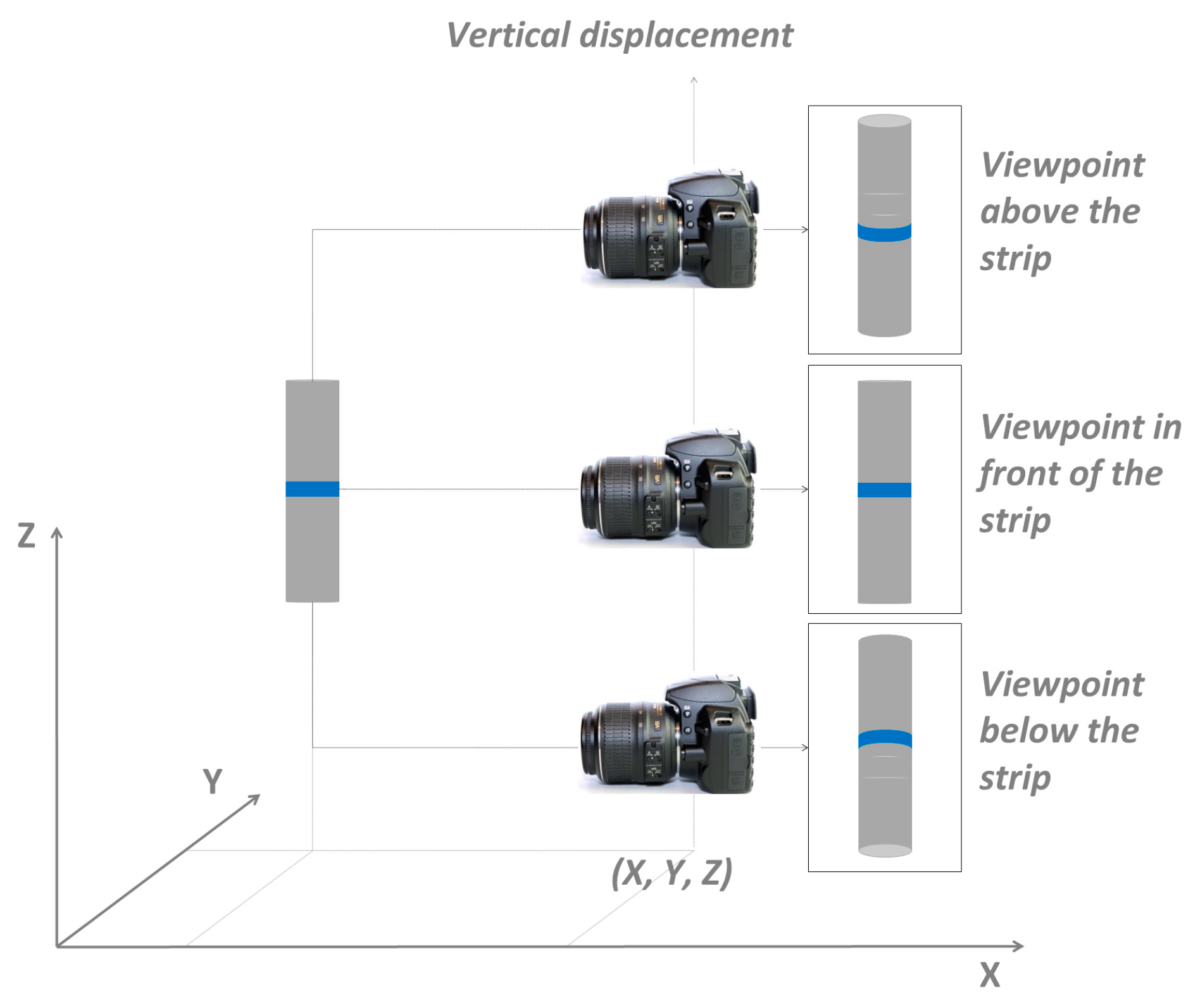
2.1. The Concept
2.2. Mathematical Model
2.3. Refinement Using ALSM
- Initial approximation between the conjugated regions with an extraction of distinguishable corresponding points (or keypoints) from the cylindrical surface. These points are used to estimate the seven parameters (ai and bi) of the geometric transformation via least squares adjustment. Some kind of texture is required to extract points that describe the surface curvature, which could be produced either by a speckle painting [33] or by structured light projection.
- From the matched points, a window is opened around the conjugated region, which covers the cylindrical diameter.
- The image coordinates of the image patch that has the curve effect is re-sampled by the transformation function that performs the first approximation of the image coordinates with a discrepancy of a few pixels.
- The correlation coefficient is computed between the image patches to determine a match point at the pixel level, although some distortions are still noticeable.
- An image matching refinement by iterative ALSM is performed to fine-tune the shape and estimate the sub-pixel coordinates of all points in the region.
- The continuous 3D reconstruction for all points inside the region is made with a photogrammetric intersection.
3. Data and Experiments
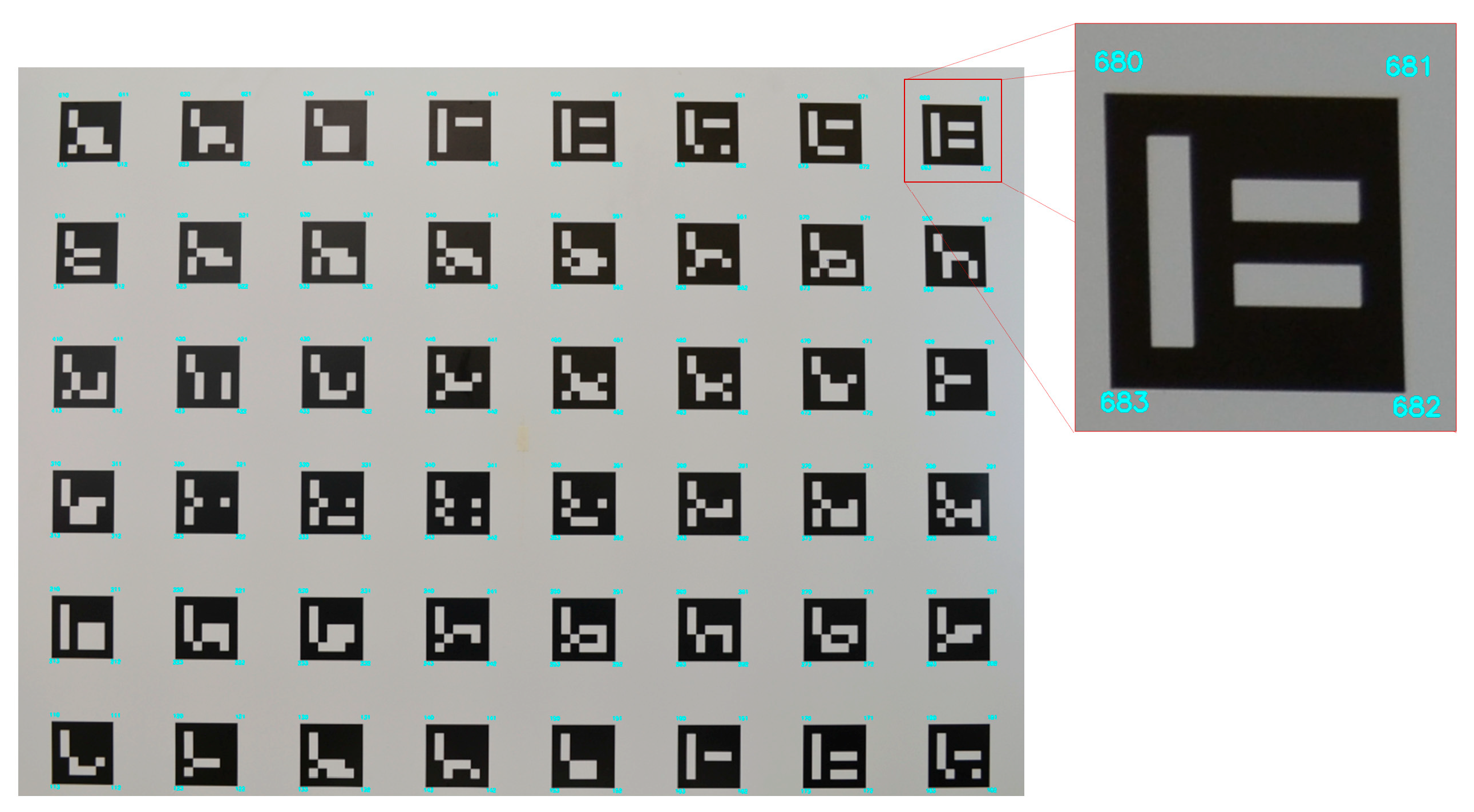
3.1. Camera Calibration
3.2. Cylinder
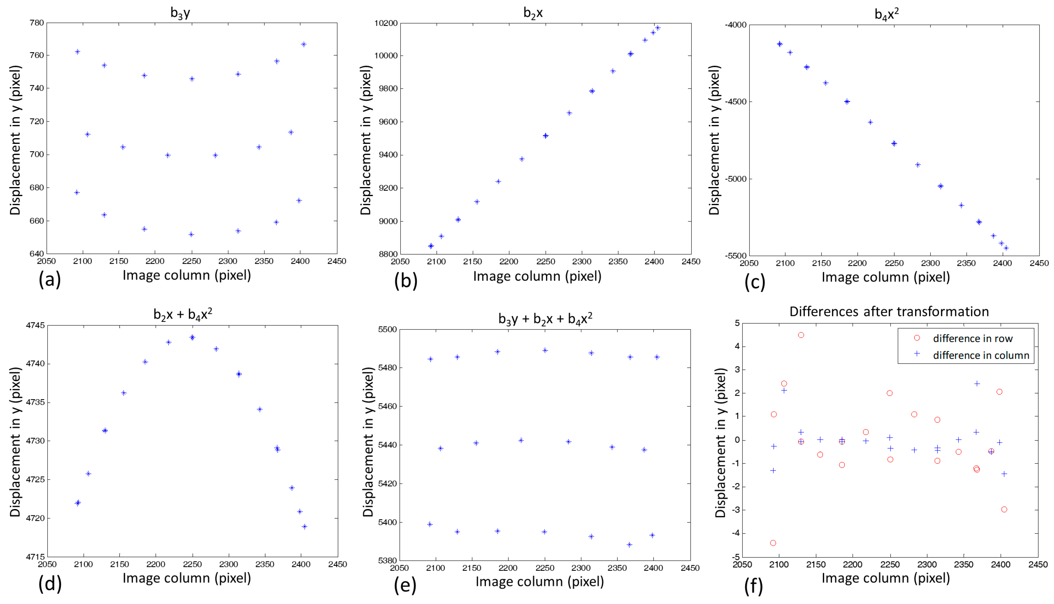
3.3. Applying Geometric Transformation
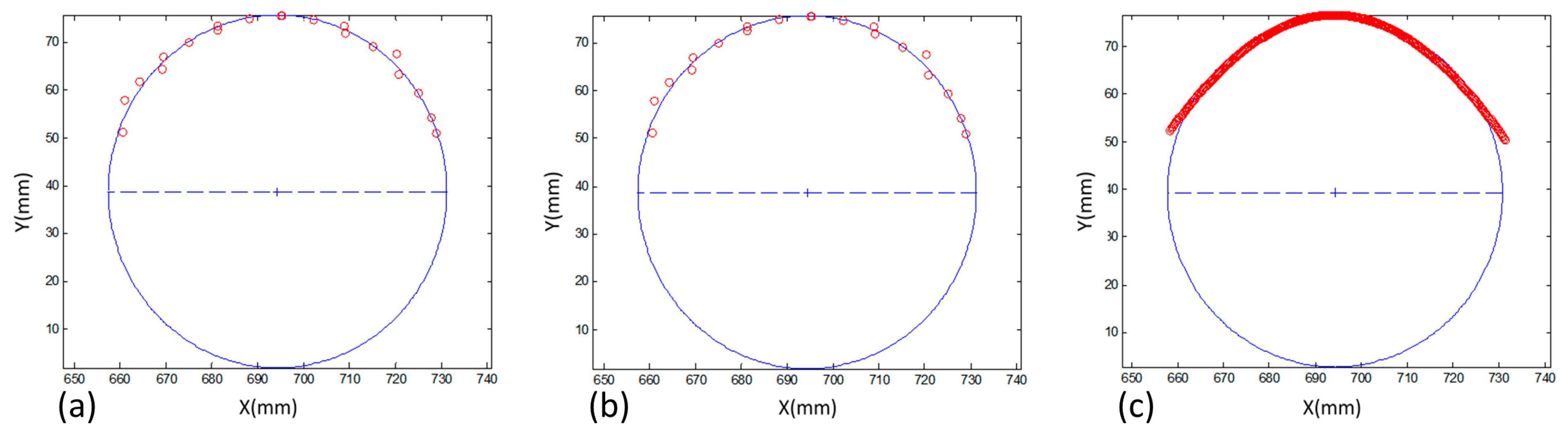
3.4. Continuous Matching for 3D Reconstruction
3.5. Textured Area
4. Analysis of the Results
- Photogrammetric intersection: using only the 3D corner coordinates determined by the intersection of rays with previously estimated extrinsic parameters.
- Bundle block adjustment (BBA): using only the 3D corner coordinates determined by bundle adjustment. In this case, the image coordinates of the corners were defined as tie points in the set of 52 images used in the camera calibration procedure.
- ALSM + intersection: using all 3D points (only planimetric coordinates) of the central line of the reconstructed strip, which were generated by a photogrammetric intersection with the proposed technique.
- For determining the geometric transformation function, a narrow strip that covers the cylindrical circumference is sufficient.
- Points extracted from the surface for image matching should be distributed along the cylindrical width for modelling its curvature.
- Points extracted for image matching should not be aligned to better estimate the geometric transformation parameters.
5. Conclusions
Author Contributions
Funding
Acknowledgments
Conflicts of Interest
References
- Furukawa, Y.; Ponce, J. Accurate, Dense, and Robust Multi-View Stereopsis. IEEE Trans. Pattern Anal. Mach. Intell. PAMI 2010, 32, 1362–1376. [Google Scholar] [CrossRef] [PubMed]
- Shan, S.M.; Adams, R.; Curless, B.; Furukawa, Y.; Sietz, S.M. The visual Turing test for scene reconstruction. In Proceedings of the Vision Conference, Seattle, WA, USA, 29 June–1 July 2013; pp. 25–32. [Google Scholar]
- Snavely, N.; Seitz, S.M.; Szeliski, R. Modeling the World from Internet Photo Collections. Int. J. Comput. Vis. 2008, 80, 189–210. [Google Scholar] [CrossRef]
- Hermann, S.; Klette, R. Iterative Semi-Global Matching for Robust Driver Assistance Systems. In Proceedings of the Computer Vision—ACCV 2012: 11th Asian Conference on Computer Vision, Daejeon, Korea, 5–9 November 2012; Lee, K.M., Matsushita, Y., Rehg, J.M., Hu, Z., Eds.; Revised Selected Papers, Part III. Springer: Berlin/Heidelberg, Germany, 2013; pp. 465–478, ISBN 978-3-642-37431-9. [Google Scholar]
- Hirschmüller, H. Stereo Processing by Semiglobal Matching and Mutual Information. IEEE Trans. Pattern Anal. Mach. Intell. 2008, 30, 328–341. [Google Scholar] [CrossRef] [PubMed]
- Remondino, F.; El-Hakim, S.F.; Gruen, A.; Zhang, L. Turning images into 3D models—Development and performance analysis of image matching for detailed surface reconstruction of heritage objects. IEEE Signal Process. Mag. 2008, 25, 55–65. [Google Scholar] [CrossRef]
- Vu, H.-H.; Labatut, P.; Pons, J.-P.; Keriven, R. High Accuracy and Visibility-Consistent Dense Multiview Stereo. IEEE Trans. Pattern Anal. Mach. Intell. 2012, 34, 889–901. [Google Scholar] [CrossRef] [PubMed]
- Potje, G.; Resende, G.; Campos, M.; Nascimento, E.R. Towards an efficient 3D model estimation methodology for aerial and ground images. Mach. Vis. Appl. 2017, 28, 937–952. [Google Scholar] [CrossRef]
- Ge, X.; Wunderlich, T. Surface-based matching of 3D point clouds with variable coordinates in source and target system. ISPRS J. Photogramm. Remote Sens. 2016, 111, 1–12. [Google Scholar] [CrossRef]
- Harwin, S.; Lucieer, A. Assessing the accuracy of georeferenced point clouds produced via multi-view stereopsis from unmanned aerial vehicle (UAV) imagery. Remote Sens. 2012, 4, 1573–1599. [Google Scholar] [CrossRef]
- Kalarot, R.; Morris, J.; Berry, D.; Dunning, J. Analysis of Real-Time Stereo Vision Algorithms on GPU. In Proceedings of the International Conference Image and Vision Computing New Zealand (IVCNZ), Auckland, New Zealand, 29 November–1 December 2011; pp. 179–184. [Google Scholar]
- Birchfield, S.; Tomasi, C. Depth discontinuities by pixel-to-pixel stereo. In Proceedings of the Sixth International Conference on Computer Vision, Bombay, India, 7 January 1998; pp. 1073–1080. [Google Scholar]
- Roy, S.; Cox, I.J. A maximum-flow formulation of the N-camera stereo correspondence problem. In Proceedings of the Sixth International Conference on Computer Vision, Bombay, India, 7 January 1998; pp. 492–499. [Google Scholar]
- Kolmogorov, V.; Criminisi, A.; Blake, A.; Cross, G.; Rother, C. Probabilistic fusion of stereo with color and contrast for bilayer segmentation. IEEE Trans. Pattern Anal. Mach. Intell. 2006, 28, 1480–1492. [Google Scholar] [CrossRef] [PubMed]
- Remondino, F.; Spera, M.G.; Nocerino, E.; Menna, F.; Nex, F. State of the arte in high density image matching. Photogramm. Rec. 2014, 29, 144–166. [Google Scholar] [CrossRef]
- Förstner, W. On the geometric precision of digital correlation. Int. Arch. Photogramm. Remote Sens. 1982, 24, 176–189. [Google Scholar]
- Ackermann, F. Digital image correlation: Performance and potential application in photogrammetry. Photogramm. Rec. 1984, 11, 429–439. [Google Scholar] [CrossRef]
- Gruen, A.W. Adaptive least squares correlation: A powerful image matching technique. S. Afr. J. Photogramm. Remote Sens. Cartogr. 1985, 14, 175–187. [Google Scholar]
- Gruen, A. Least square matching: A fundamental measurement algorithm. In Close Range Photogrammetry and Machine Vision; Whittle Publishing: Bristol, UK, 1996; pp. 217–255. [Google Scholar]
- Gruen, A.W.; Baltsavias, E.P. Geometrically constrained multiphoto matching. Photogramm. Eng. Remote Sens. 1988, 54, 633–641. [Google Scholar]
- Müller, H. Designing an object-oriented matching tool. Int. Arch. Photogramm. Remote Sens. 1997, 32, 120–127. [Google Scholar]
- Bethmann, F.; Luhmann, T. Least-squares Matching with Advanced Geometric Transformation Models. Photogramm. Fernerkund. Geoinf. 2011, 2011, 57–69. [Google Scholar] [CrossRef]
- Zhang, Y.; Xiong, J.; Hao, L. Photogrammetric processing of low-altitude images acquired by unpiloted aerial vehicles. Photogramm. Rec. 2011, 26, 190–211. [Google Scholar] [CrossRef]
- Debella-Gilo, M.; Kääb, A. Measurement of Surface Displacement and Deformation of Mass Movements Using Least Squares Matching of Repeat High Resolution Satellite and Aerial Images. Remote Sens. 2012, 4, 43–67. [Google Scholar] [CrossRef]
- Schewe, H.; Förstner, W. The program PALM for automatic line and surface measurement using image matching techniques. Int. Arch. Photogramm. Remote Sens. 1986, 26, 608–622. [Google Scholar]
- Bartelsen, J.; Mayer, H.; Hirschmüller, H.; Kuhn, A.; Michelini, M. Orientation and Dense Reconstruction from Unordered Wide Baseline Image Sets. PFG Photogramm. Fernerkund. Geoinf. 2012, 2012, 421–432. [Google Scholar] [CrossRef]
- Gong, J.; Li, Z.; Zhu, Q.; Sui, H.; Zhou, Y. Effects of various factors on the accuracy of DEMs: An intensive experimental investigation. Photogramm. Eng. Remote Sens. 2000, 66, 1113–1117. [Google Scholar]
- Kersten, T.P.; Lindstaedt, M. Automatic 3D Object Reconstruction from Multiple Images for Architectural, Cultural Heritage and Archaeological Applications Using Open-Source Software and Web Services. PFG Photogramm. Fernerkund. Geoinf. 2012, 2012, 727–740. [Google Scholar] [CrossRef]
- Remondino, F.; Menna, F. Image-based surface measurement for close-range heritage documentation. Int. Arch. Photogramm. Remote Sens. Spat. Inf. Sci. 2008, 37, 199–206. [Google Scholar]
- Smith, M.J.; Smith, D.G. Operational experiences of digital photogrammetric systems. Int. Arch. Photogramm. Remote Sens. Spat. Inf. Sci. 1996, 31, 357–362. [Google Scholar]
- Xu, X.; Zhang, Q.; Su, Y.; Cai, Y.; Xue, W.; Gao, Z.; Xue, Y.; Lv, Z.; Fu, S. High-Accuracy, High-Efficiency Compensation Method in Two-Dimensional Digital Image Correlation. Exp. Mech. 2017, 57, 831–846. [Google Scholar] [CrossRef]
- Wang, Y.-Q.; Sutton, M.A.; Ke, X.-D.; Schreier, H.W.; Reu, P.L.; Miller, T.J. On Error Assessment in Stereo-based Deformation Measurements. Exp. Mech. 2011, 51, 405–422. [Google Scholar] [CrossRef]
- Pan, B.; Li, K.; Tong, W. Fast, Robust and Accurate Digital Image Correlation Calculation Without Redundant Computations. Exp. Mech. 2013, 53, 1277–1289. [Google Scholar] [CrossRef]
- Harvent, J.; Coudrin, B.; Brethes, L.; Orteu, J.-J. Shape measurement using anew multi-step stereo-DIC algorithm that preserves sharp edges. Exp. Mech. 2015, 55, 167–176. [Google Scholar] [CrossRef]
- Nixon, C.A.; Marcum, W.R.; Steer, K.M.; Jackson, R.B. A New Method for Experimentally Quantifying Dynamic Deflection of a Cylindrical Structure. Exp. Mech. 2018. [Google Scholar] [CrossRef]
- Seitz, S.M.; Curless, B.; Diebel, J.; Scharstein, D.; Szeliski, R. A Comparison and Evaluation of Multi-View Stereo Reconstruction Algorithms. In Proceedings of the 2006 IEEE Computer Society Conference on Computer Vision and Pattern Recognition (CVPR ’06), New York, NY, USA, 17–22 June 2006; IEEE Computer Society: Washington, DC, USA, 2006; Volume 1, pp. 519–528. [Google Scholar]
- Sutton, M.A.; Matta, F.; Rizos, D.; Ghorbani, R.; Rajan, S.; Mollenhauer, D.H.; Schreier, H.W.; Lasprilla, A.O. Recent Progress in Digital Image Correlation: Background and Developments since the 2013 W M Murray Lecture. Exp. Mech. 2017, 57, 1–30. [Google Scholar] [CrossRef]
- Mikhail, E.M.; Bethel, J.S.; McGlone, C.J. Introduction to Modern Photogrammetry; John Wiley & Sons Inc.: New York, NY, USA, 2001. [Google Scholar]
- Garrido-Jurado, S.; Muñoz-Salinas, R.; Madrid-Cuevas, F.J.; Marín-Jiménez, M.J. Automatic generation and detection of highly reliable fiducial markers under occlusion. Pattern Recognit. 2014, 47, 2280–2292. [Google Scholar] [CrossRef]
- Tommaselli, A.M.G.; Marcato, J., Jr.; Moraes, M.V.A.; Silva, S.L.A.; Artero, A.O. Calibration of panoramic cameras with coded targets and a 3D calibration field. ISPRS Int. Arch. Photogramm. Remote Sens. Spat. Inf. Sci. 2014, XL-3/W1, 137–142. [Google Scholar] [CrossRef]
- Kenefick, J.F.; Gyer, M.S.; Harp, B.F. Analytical self-calibration. Photogramm. Eng. 1972, 38, 1117–1126. [Google Scholar]
- Ruy, R.; Tommaselli, A.M.G.; Galo, M.; Hasegawa, J.K.; Reis, T.T. Evaluation of bundle block adjustment with additional parameters using images acquired by SAAPI system. In Proceedings of the 6th International Symposium on Mobile Mapping Technology, Presidente Prudente, Brazil, 21–24 July 2009. [Google Scholar]
- Fryer, J.G.; Brown, D.C. Lens Distortion for Close-Range Photogrammetry. Photogramm. Eng. Remote Sens. 1986, 52, 51–58. [Google Scholar]
- Stamatopoulos, C.; Chuang, T.Y.; Fraser, C.S.; Lu, Y.Y. Fully automated image orientation in the absence of targets. Int. Arch. Photogramm. Remote Sens. Spat. Inf. Sci. 2012, XXXIX-B5, 303–308. [Google Scholar] [CrossRef]
- Förstner, W.; Gülch, E. A fast operator for detection and precise location of distinct points, corners and centres of circular features. In Proceedings of the ISPRS Intercommission Conference on Fast Processing of Photogrammetric Data, Interlaken, Switzerland, 2–4 June 1987; pp. 281–305. [Google Scholar]
- Lowe, D.G. Distinctive Image Features from Scale-Invariant Keypoints. Int. J. Comput. Vis. 2004, 60, 91–110. [Google Scholar] [CrossRef]


| Feature | Specification |
|---|---|
| Digital camera model | Nikon D3100 |
| Sensor size | CMOS APS-C (23.1 mm × 15.4 mm) |
| Image dimensions | 4608 × 3072 pixels |
| Pixel size | 5 μm |
| Nominal focal length | 24 mm (AF-S DX Nikkor) |
| a1 (pixel) | a2 | a3 | b1 (pixel) | b2 | b3 | b4 |
|---|---|---|---|---|---|---|
| −72.0392 | 1.0112 | −0.0057 | −3698.0498 | 4.2292 | 1.0228 | −0.0009 |
| Part | a1 | a2 | a3 | b1 | b2 | b3 | b4 |
|---|---|---|---|---|---|---|---|
| Patch I | −78.9782 | 1.0018 | 0.0510 | −2582.1701 | 3.2421 | 0.9983 | −0.0007 |
| Patch II | −95.1206 | 1.0085 | 0.0297 | −2522.9268 | 3.2021 | 1.0013 | −0.0007 |
| Photogrammetric Technique | Standard Deviation (mm) | Difference between Diameters (mm) | ||
|---|---|---|---|---|
| σXc | σYc | σdiameter | ||
| Intersection | 0.3016 | 0.8686 | 0.6773 | 0.20 |
| BBA | 0.3019 | 0.8697 | 0.6782 | 0.27 |
| ALSM + Intersection | 0.0702 | 0.1984 | 0.1623 | 0.13 |
| Textured Area | Standard Deviation (mm) | Diameter Error (mm) | ||
|---|---|---|---|---|
| σXc | σYc | σdiameter | ||
| Part I—only SIFT keypoints | 0.3286 | 1.4588 | 1.2308 | 0.0030 |
| Part II—only SIFT keypoints | 0.3708 | 2.0669 | 1.7389 | 0.0079 |
| Part I—ALSM | 0.0702 | 0.1983 | 0.1622 | 0.0001 |
| Part II—ALSM | 0.0302 | 0.1038 | 0.0916 | 0.0033 |
| Cylinder | Length (mm) | Measured Diameter (mm) | Standard Deviation (mm) | Diameter Error (mm) | ||
|---|---|---|---|---|---|---|
| σXc | σYc | σdiameter | ||||
| I | 170 | 31.702 | 0.028 | 0.207 | 0.207 | 0.066 |
| II | 126 | 50.622 | 0.026 | 0.083 | 0.074 | 0.050 |
© 2018 by the authors. Licensee MDPI, Basel, Switzerland. This article is an open access article distributed under the terms and conditions of the Creative Commons Attribution (CC BY) license (http://creativecommons.org/licenses/by/4.0/).
Share and Cite
Berveglieri, A.; Tommaselli, A.M.G. Reconstruction of Cylindrical Surfaces Using Digital Image Correlation. Sensors 2018, 18, 4183. https://doi.org/10.3390/s18124183
Berveglieri A, Tommaselli AMG. Reconstruction of Cylindrical Surfaces Using Digital Image Correlation. Sensors. 2018; 18(12):4183. https://doi.org/10.3390/s18124183
Chicago/Turabian StyleBerveglieri, Adilson, and Antonio M. G. Tommaselli. 2018. "Reconstruction of Cylindrical Surfaces Using Digital Image Correlation" Sensors 18, no. 12: 4183. https://doi.org/10.3390/s18124183
APA StyleBerveglieri, A., & Tommaselli, A. M. G. (2018). Reconstruction of Cylindrical Surfaces Using Digital Image Correlation. Sensors, 18(12), 4183. https://doi.org/10.3390/s18124183