Design and Evaluation of a Structural Analysis-Based Fault Detection and Identification Scheme for a Hydraulic Torque Converter

Abstract
1. Introduction
2. Hazard Analysis of the Hydraulic Torque Converter
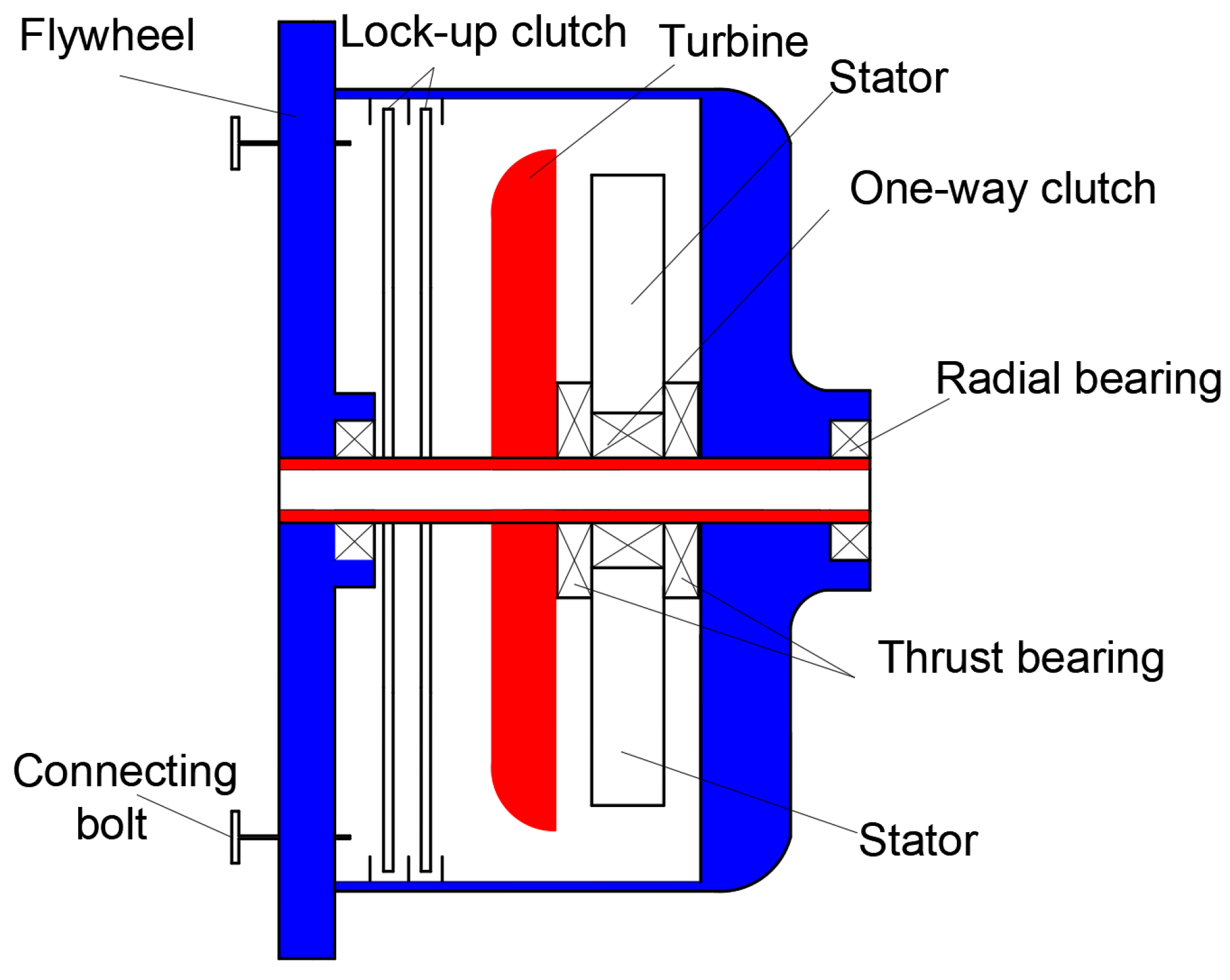
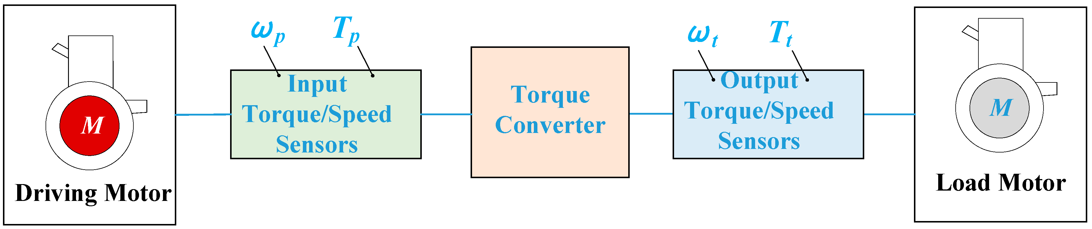
2.1. Basic Structure and Function of the HTC
2.2. Fault Mode and Effect Analysis (FMEA) of the HTC
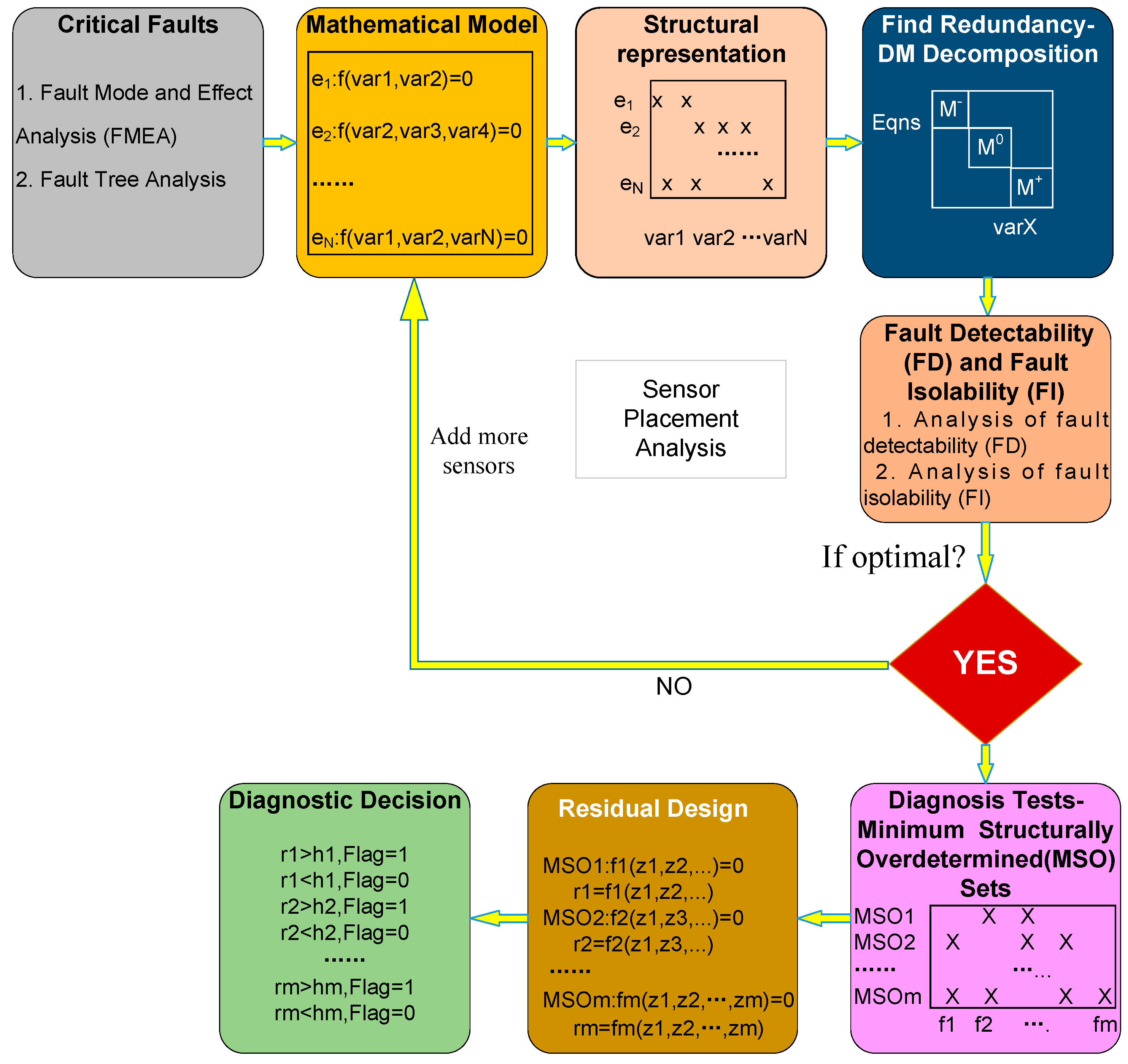
3. Fault Diagnosis of the Hydraulic Torque Converter via Structural Analysis
3.1. Fault Modeling of the HTC
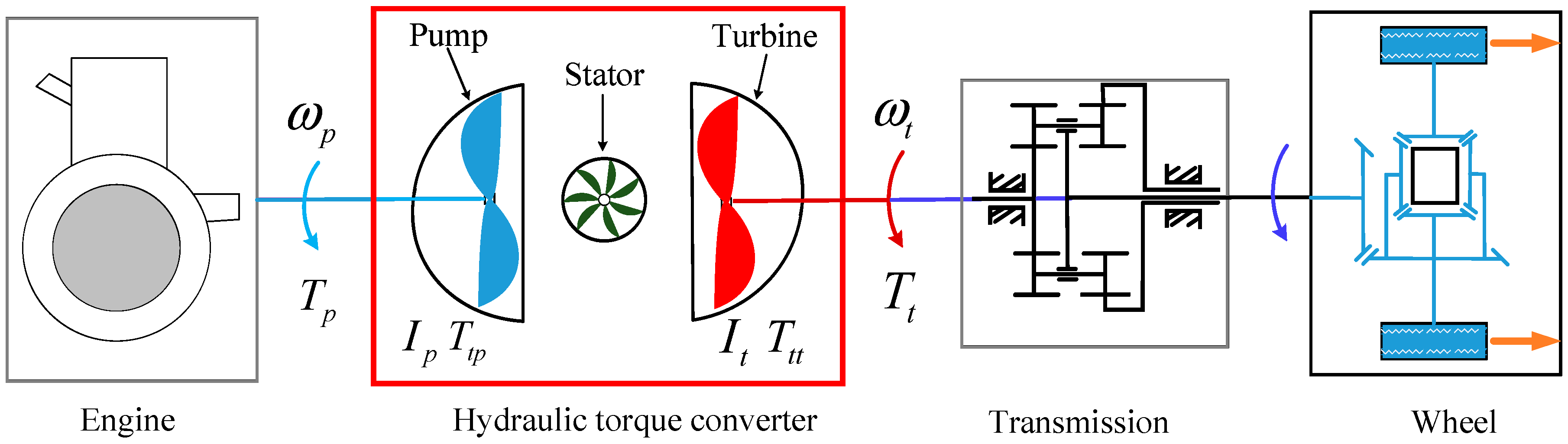
3.1.1. Mathematical Model of the HTC
3.1.2. Fault Modelling of the HTC
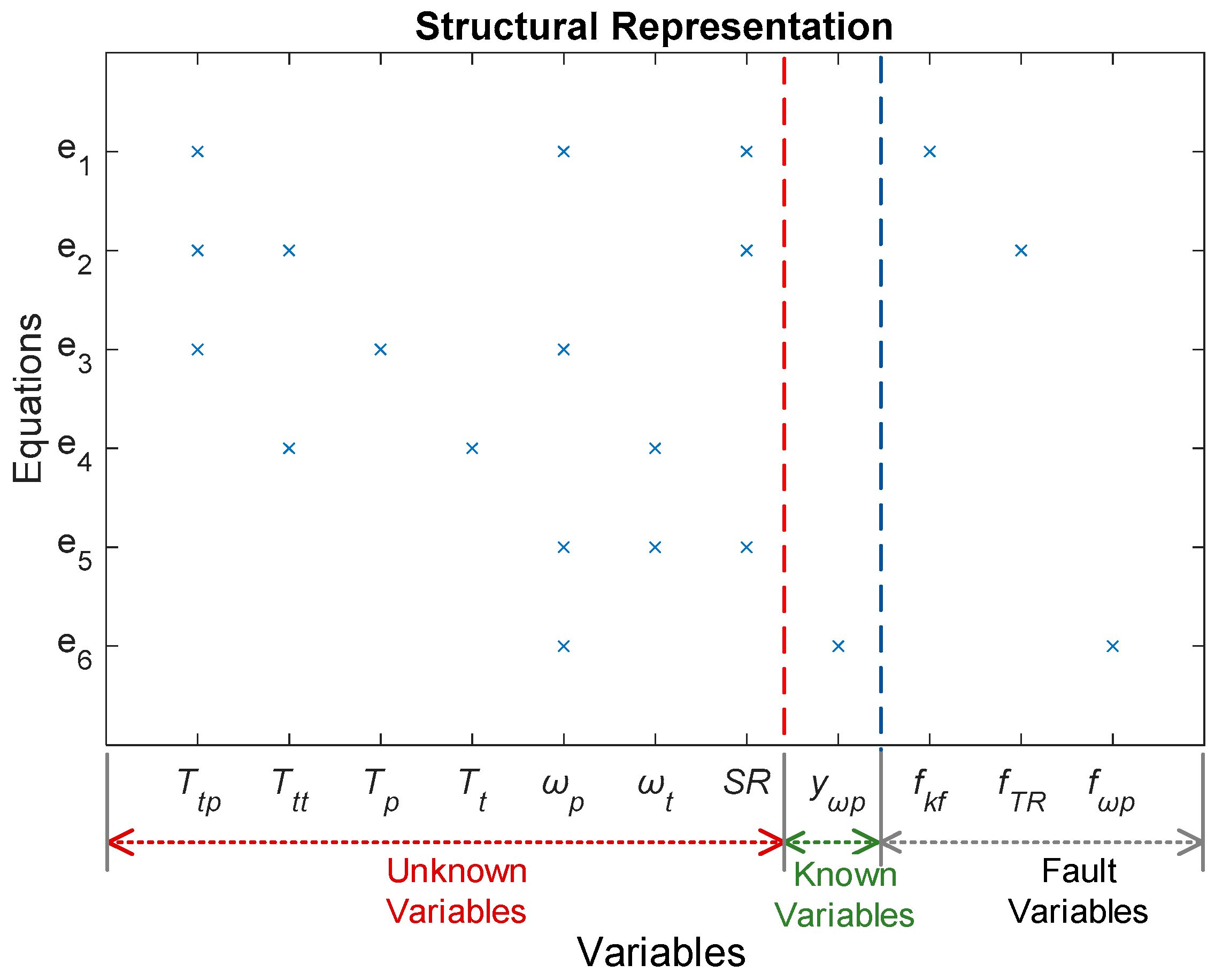
3.2. Structural Representation of the HTC
- Unknown variables:
- Known variables:
- Fault variables:
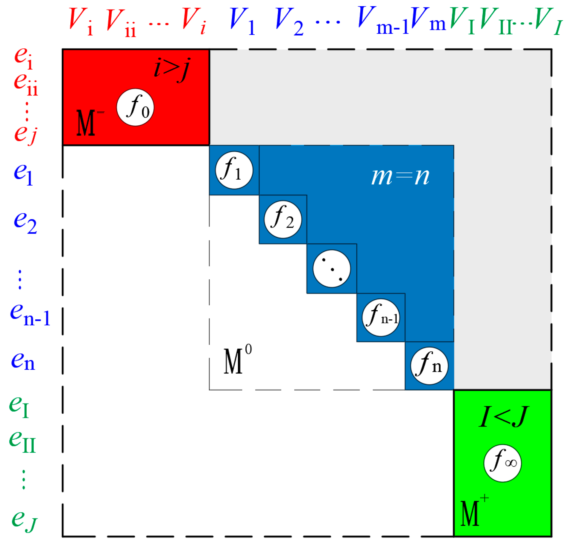
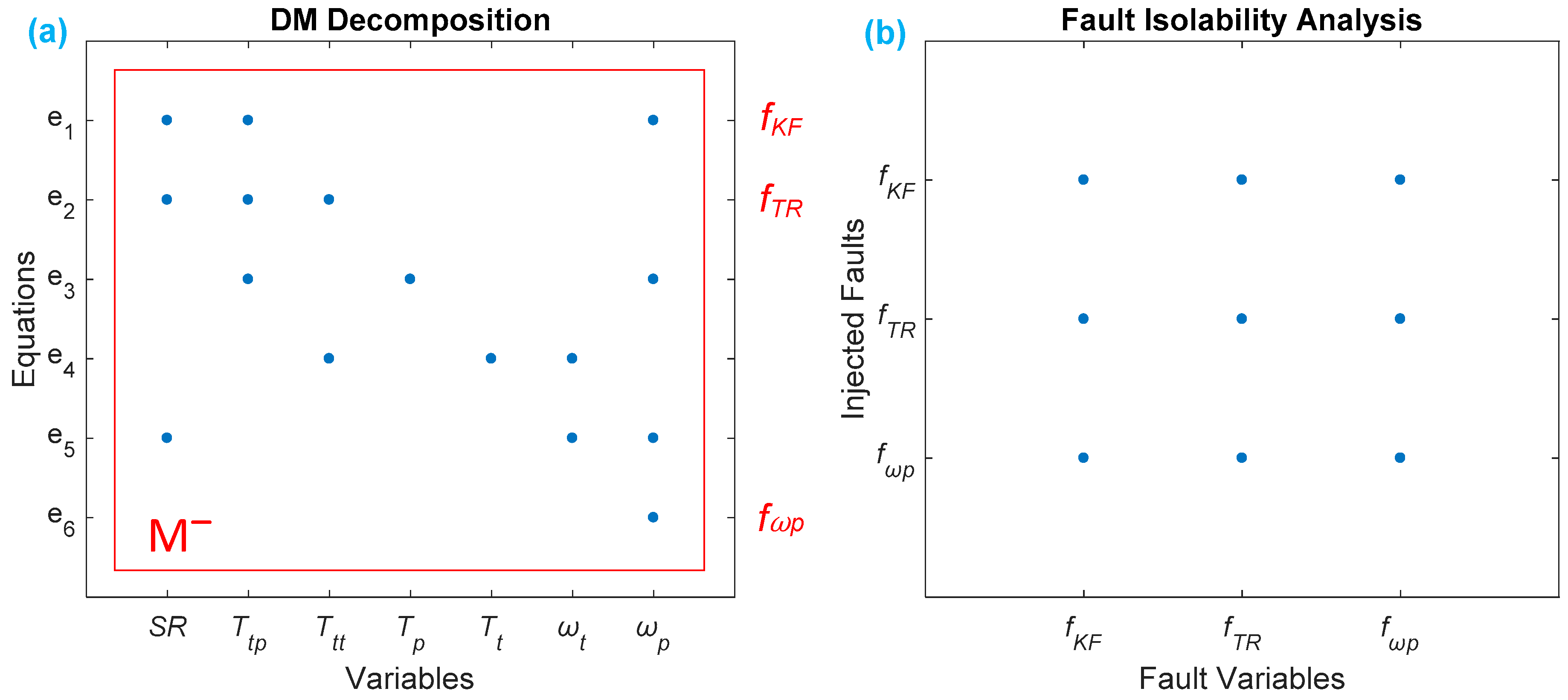
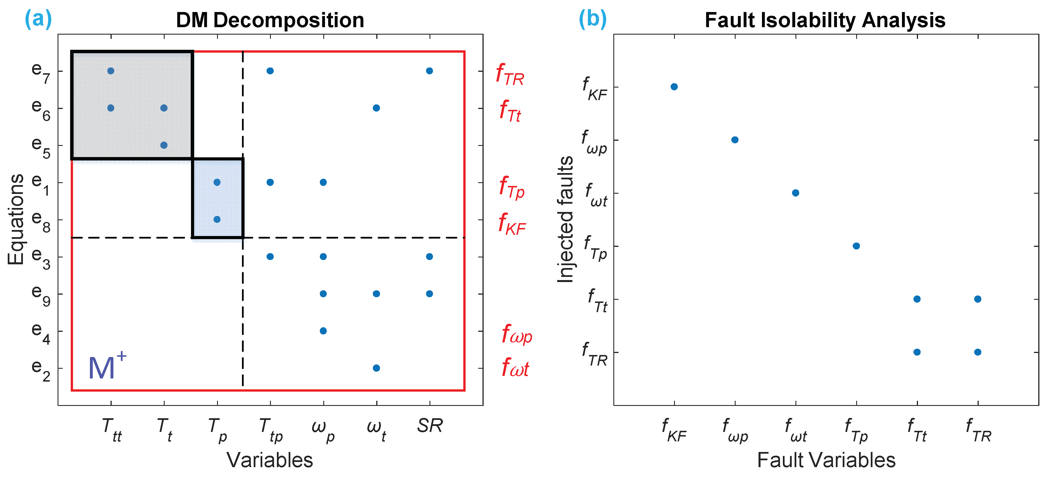
3.3. Analysis of Fault Detectability and the Isolability of the HTC
3.3.1. Fault Detectability Analysis
3.3.2. Fault Isolability Analysis
3.4. Sensor Placement for the HTC
3.5. Finding MSO Sets
3.6. Residual Design
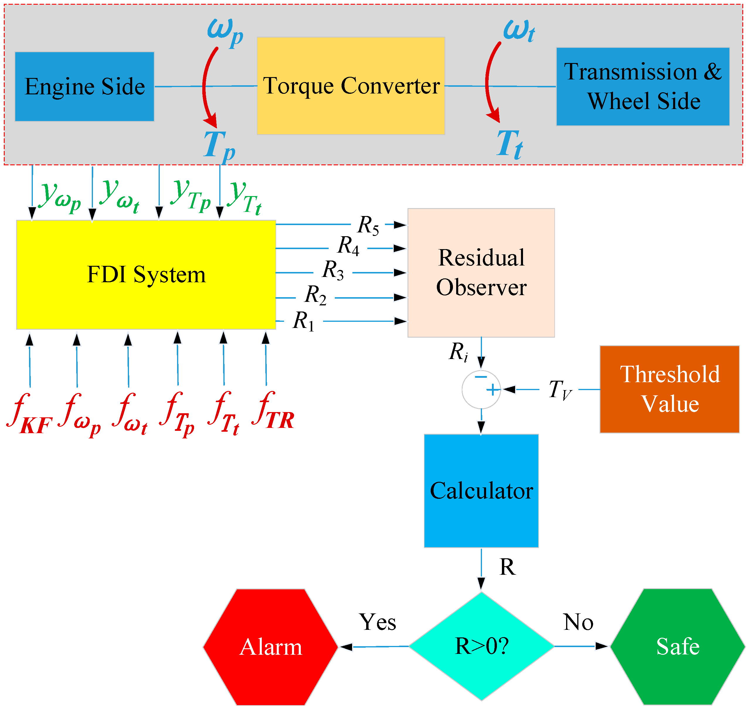
4. Design and Validation of the FDI System for the HTC
4.1. Establishment of the FDI System
4.2. Validation of the FDI System for the HTC
4.2.1. Fault Setting
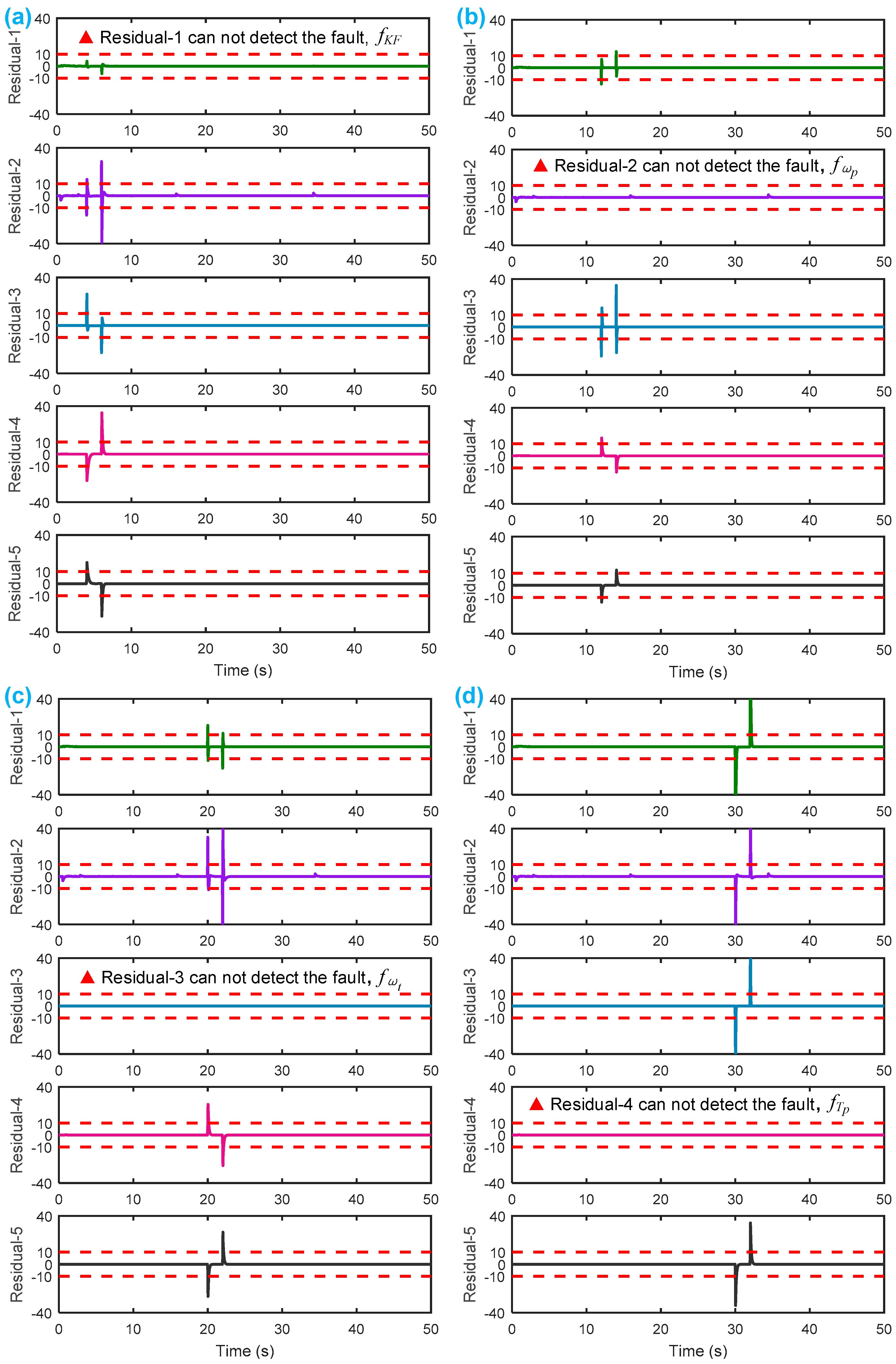
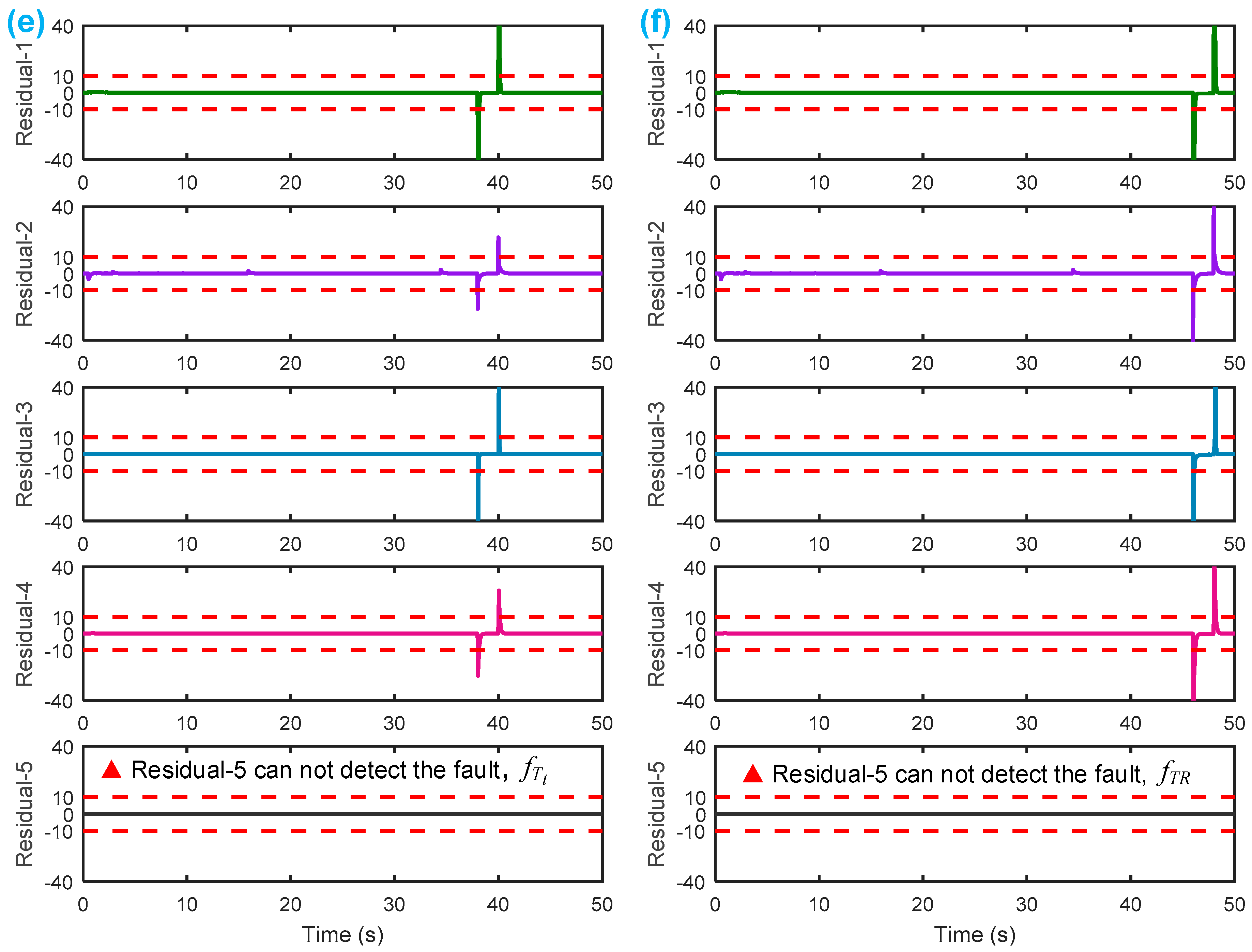
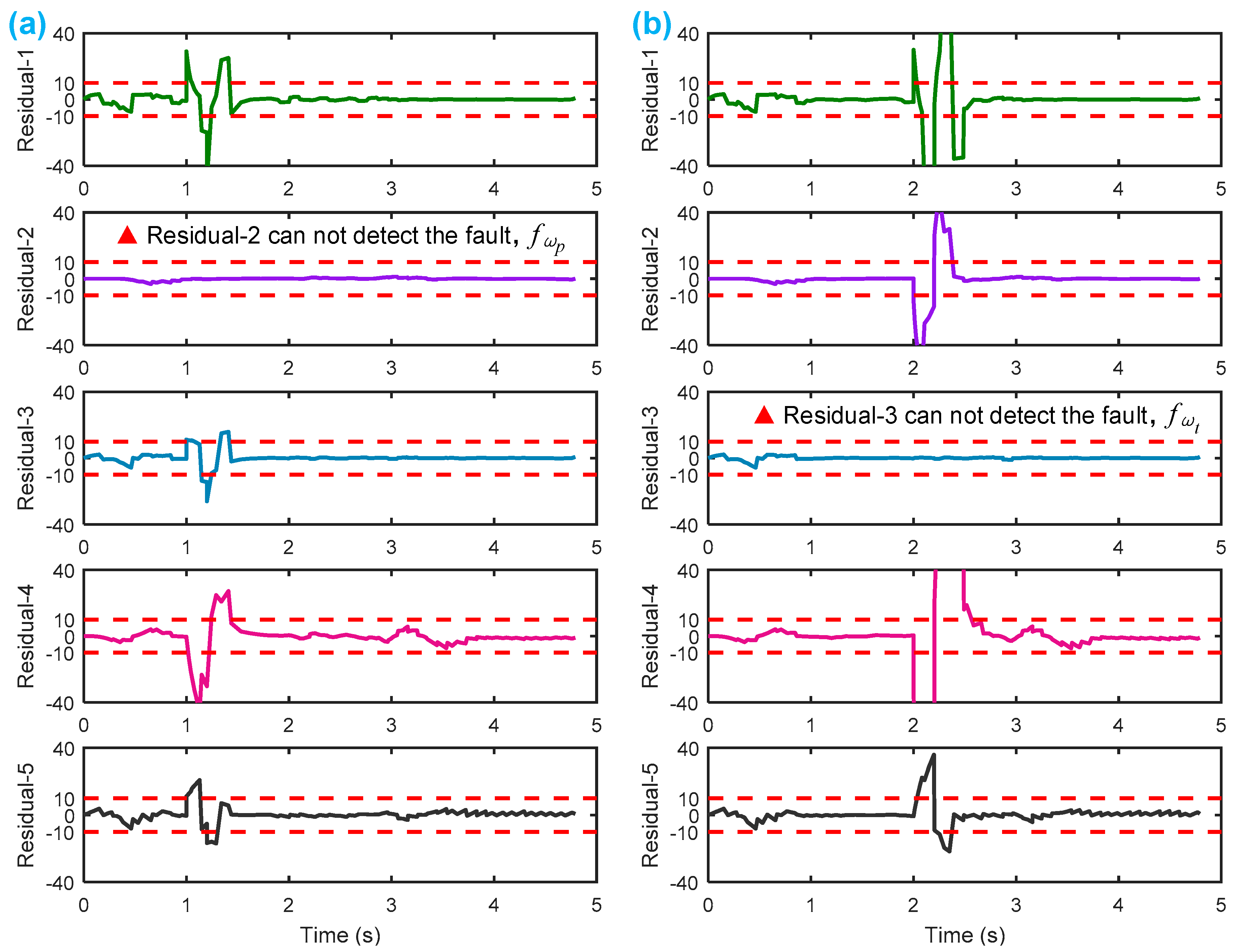
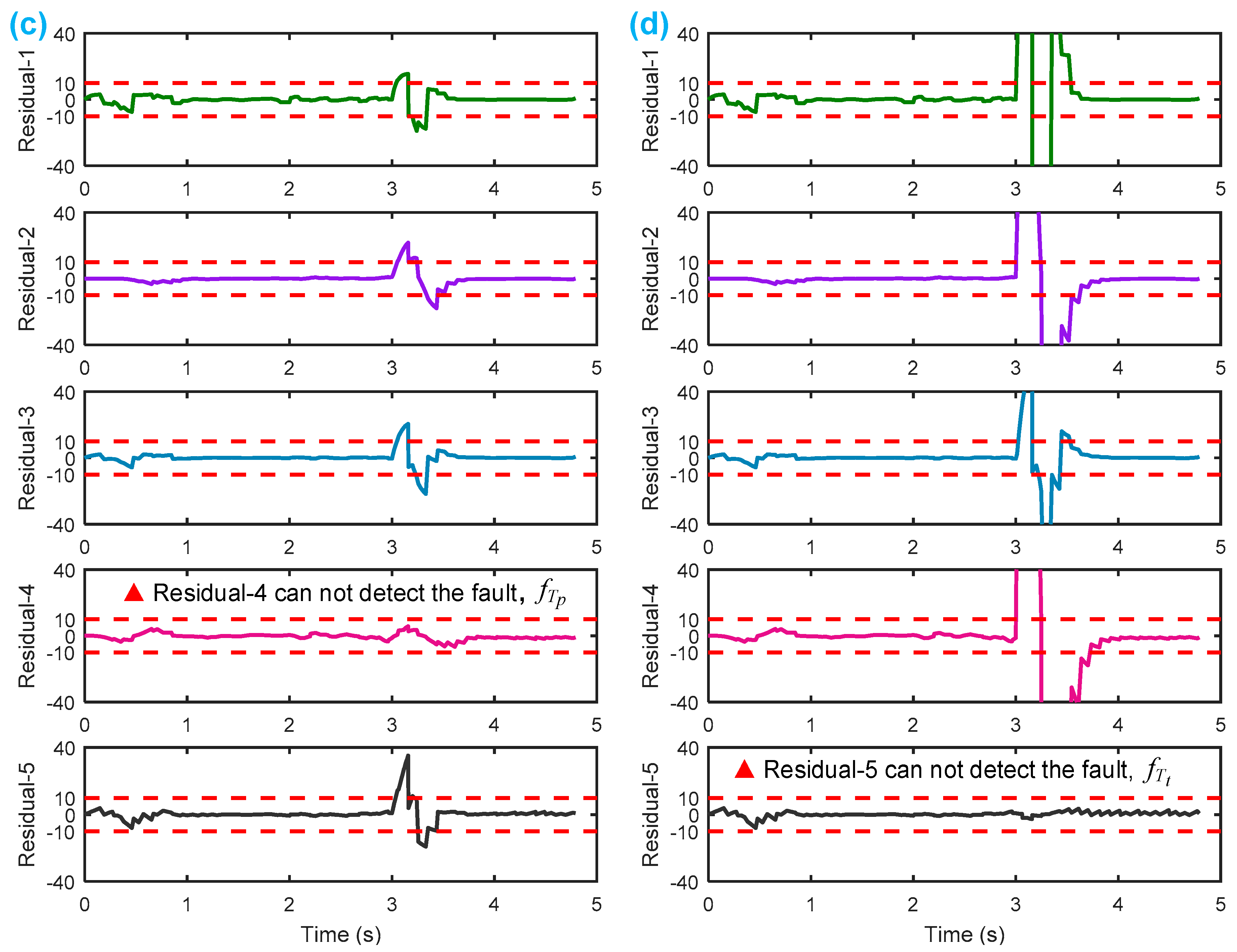
4.2.2. Simulation and Discussion of the FDI System
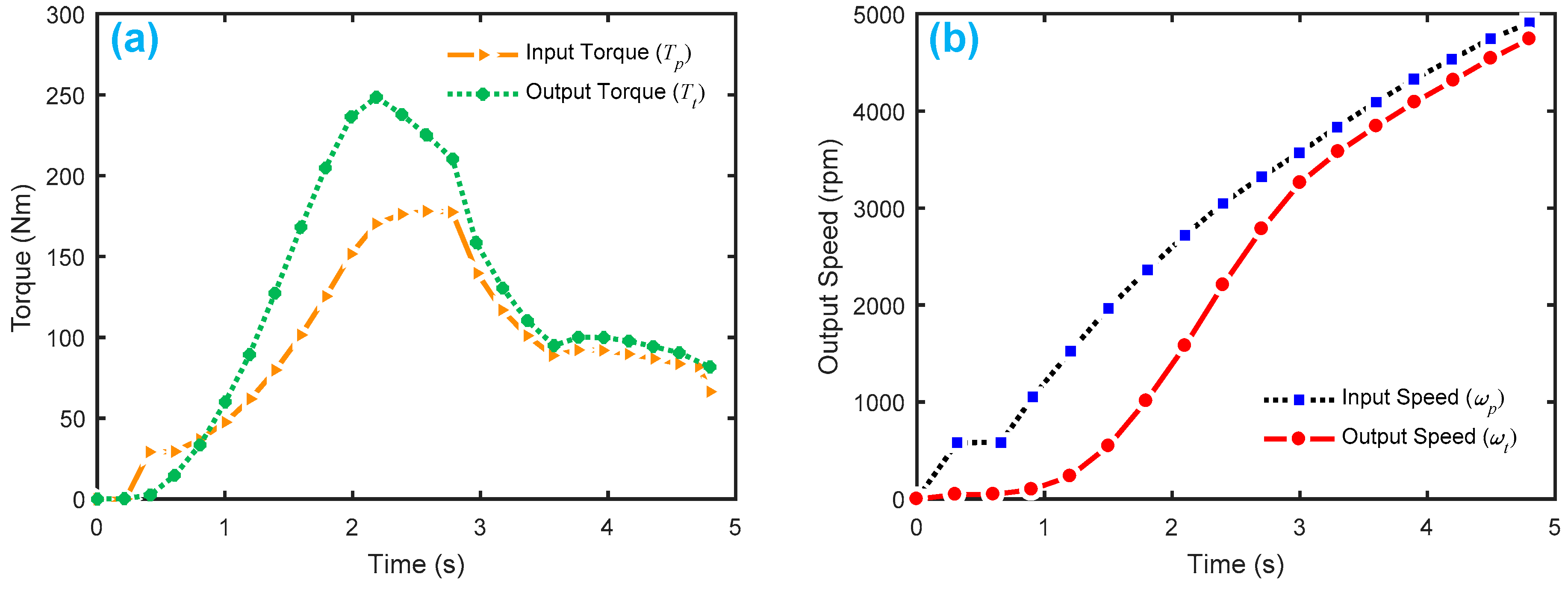
5. Experimental Validation
6. Conclusions
Author Contributions
Funding
Acknowledgments
Conflicts of Interest
List of Symbols
| critical fault lying in pump group | |
| critical fault lying in turbine group | |
| fault of pump torque | |
| fault of turbine torque | |
| fault of engine angular velocity | |
| fault of pump angular velocity | |
| fault of turbine angular velocity | |
| fault of wheel angular velocity | |
| inertia of the pump | |
| pump inertia of HTC in Honda CRV | |
| inertia of the turbine | |
| turbine inertia of HTC in Honda CRV | |
| equivalent inertia of vehicle | |
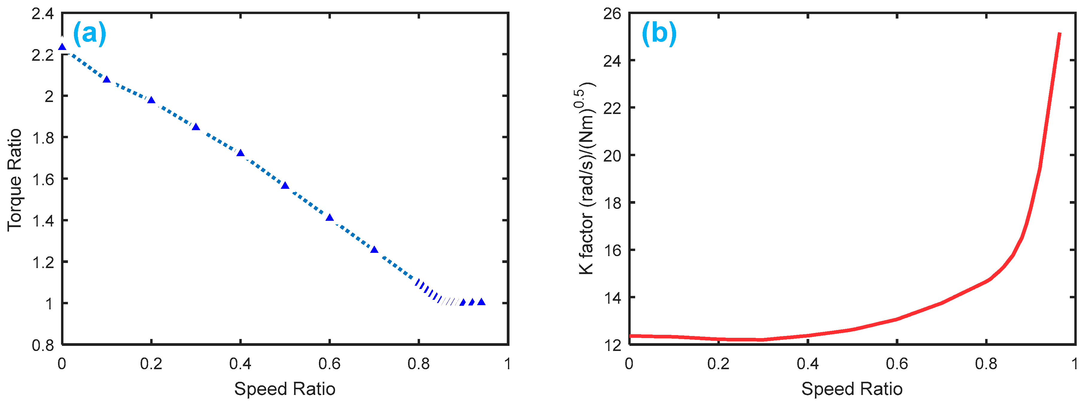
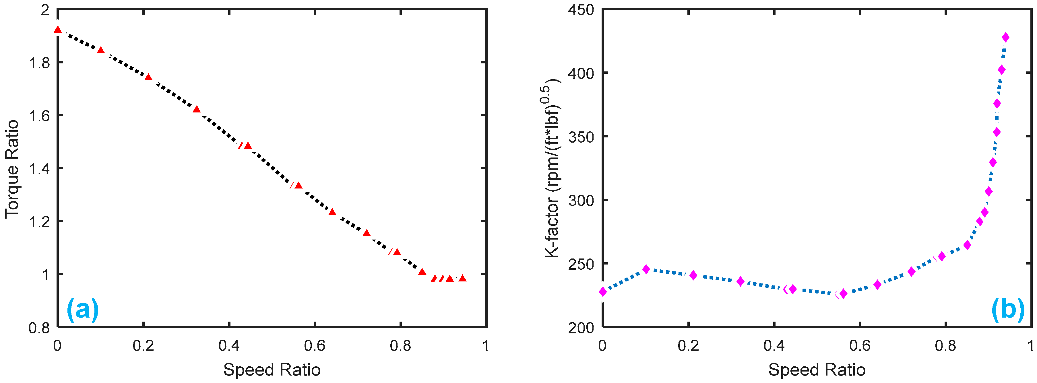
| KF | K-factor |
| SR | speed ratio |
| torque in the pump | |
| turbine output torque | |
| TR | torque ratio |
| torque transferred by the pump | |
| torque transferred by the turbine | |
| pump wheel angular velocity | |
| turbine angular velocity | |
| measurement of pump torque | |
| measurement of turbine torque | |
| measurement of pump angular velocity | |
| measurement of turbine angular velocity | |
| variables in the residuals of simulation | |
| variables in the residuals of experiment |
References
- Palin, R.; Ward, D.; Habli, I.; Rivett, R. ISO 26262 safety cases: Compliance and assurance. In Proceedings of the 6th IET International Conference on System Safety, Birmingham, UK, 20–22 September 2011. [Google Scholar]
- Kesy, A. Mathematical model of a Hydrodynamic Torque Converter for vehicle power transmission system optimisation. Int. J. Veh. Des. 2012, 59, 1–22. [Google Scholar] [CrossRef]
- Mishra, K.D.; Srinivasan, K. On-line identification of a torque converter model. IFAC-PapersOnLine 2017, 50, 4763–4768. [Google Scholar] [CrossRef]
- Hahn, J.-O.; Lee, K.-I. Nonlinear robust control of torque converter clutch slip system for passenger vehicles using advanced torque estimation algorithms. Veh. Syst. Dyn. 2002, 37, 175–192. [Google Scholar] [CrossRef]
- Burtch, J.B. Torque Converter Clutch Slip Control Systems and Methods Based on Active Cylinder Count. U.S. Patent 8979708, 17 March 2015. [Google Scholar]
- Dong, Y.; Korivi, V.; Attibele, P.; Yuan, Y. Torque converter CFD engineering part II: Performance improvement through core leakage flow and cavitation control. In Proceedings of the SAE 2002 World Congress & Exhibition, Detroit, MI, USA, 3–7 March 2002. [Google Scholar]
- Tsutsumi, K.; Watanabe, S.; Tsuda, S.-I.; Yamaguchi, T. Cavitation simulation of automotive torque converter using a homogeneous cavitation model. Eur. J. Mech. B Fluids 2017, 61, 263–270. [Google Scholar] [CrossRef]
- Pohl, B. Transient Torque Converter Performance, Testing, Simulation and Reverse Engineering; SAE: Warrendale, PA, USA, 2003. [Google Scholar]
- Li, Y.; Sundén, M. Modelling and Measurement of Transient Torque Converter Characteristics. Master’s Thesis, Chalmers University of Technology, Gothenburg, Sweden, 2016. [Google Scholar]
- Zhang, L.; Yueyong, C. Analysis on fault diagnosis of hydraulic torque converter of automatic transmission. Motor China 2005, 11, 72–76. (In Chinese) [Google Scholar]
- Chen, Z. Research on Fault Diagnosis Method and Diagnosis System of Automatic Transmission. Master’s Thesis, Shanghai Jiaotong University, Shanghai, China, 2007. (In Chinese). [Google Scholar]
- Li, W. New Car Automatic Transmission Structure Principle and Maintenance Case; Chemical Industry Press: Beijing, China, 2015; p. 309. (In Chinese) [Google Scholar]
- He, F.; Lin, Y.; Wang, G.Y.; Nie, R. Analysis of malfunction cause and countermeasure for hydraulic torque converter. Constr. Mach. 2010, 7, 96–97. (In Chinese) [Google Scholar]
- Zhang, Z. Model-Based Fault Diagnosis of the 6-Speed Automatic Transmission. Master’s Thesis, Hefei University of Technology, Hefei, China, 2017. (In Chinese). [Google Scholar]
- Gao, W.; Zhidong, W. Auto Automatic Transmission Maintenance Principle and Example Tutorial; China Railway Press: Beijing, China, 2014. (In Chinese) [Google Scholar]
- Wang, Z. Automobile Automatic Transmission Principle and Maintenance Integration Tutorial; Mechanical Industry Press: Beijing, China, 2009. (In Chinese) [Google Scholar]
- Wang, N.; Chen, J.; Han, J.; Liu, J.; Guo, X. Application of Fault Diagnosis Technology in Hydraulic Torque Converter Test Bench. Tract. Farm Transp. 2018, 45, 15–16. (In Chinse) [Google Scholar]
- Isermann, R. Model-based fault-detection and diagnosis–status and applications. Annu. Rev. Control 2005, 29, 71–85. [Google Scholar] [CrossRef]
- Zhang, J. Model-Based Fault Diagnosis for Automotive Functional Safety. Ph.D. Thesis, The Ohio State University, Columbus, OH, USA, 2016. [Google Scholar]
- Luo, J.; Pattipati, K.R.; Qiao, L.; Chigusa, S. Model-based prognostic techniques applied to a suspension system. IEEE Trans. Syst. Man Cybern. Part A 2008, 38, 1156–1168. [Google Scholar]
- Börner, M.; Straky, H.; Weispfenning, T.; Isermann, R. Model based fault detection of vehicle suspension and hydraulic brake systems. Mechatronics 2002, 12, 999–1010. [Google Scholar] [CrossRef]
- Pisu, P.; Serrani, A.; You, S.; Jalics, L. Adaptive threshold based diagnostics for steer-by-wire systems. J. Dyn. Syst. Meas. Control 2006, 128, 428–435. [Google Scholar] [CrossRef]
- Pisu, P.; Soliman, A.; Rizzoni, G. Vehicle chassis monitoring system. Control Eng. Pract. 2003, 11, 345–354. [Google Scholar] [CrossRef]
- Ghimire, R.; Sankavaram, C.; Ghahari, A.; Pattipati, K.; Ghoneim, Y.; Howell, M.; Salman, M. Integrated model-based and data-driven fault detection and diagnosis approach for an automotive electric power steering system. In Proceedings of the 2011 IEEE Autotestcon, Baltimore, MD, USA, 12–15 September 2011; pp. 70–77. [Google Scholar]
- Djeziri, M.A.; Bouamama, B.O.; Dauphin-Tanguy, G.; Merzouki, R. LFT bond graph model-based robust fault detection and isolation. In Bond Graph Modelling of Engineering Systems; Springer: Berlin, Germany, 2011; pp. 105–133. [Google Scholar]
- Broenink, J.F. Introduction to physical systems modelling with bond graphs. SiE Whitebook Simul. Methodol. 1999, 31, 1–31. [Google Scholar]
- Düştegör, D.; Frisk, E.; Cocquempot, V.; Krysander, M.; Staroswiecki, M. Structural analysis of fault isolability in the DAMADICS benchmark. Control Eng. Pract. 2006, 14, 597–608. [Google Scholar] [CrossRef]
- Krysander, M.; Frisk, E. Sensor placement for fault diagnosis. IEEE Trans. Syst. Man Cybern. Part A 2008, 38, 1398–1410. [Google Scholar] [CrossRef]
- Frisk, E.; Krysander, M.; Jung, D. A toolbox for analysis and design of model based diagnosis systems for large scale models. IFAC-PapersOnLine 2017, 50, 3287–3293. [Google Scholar] [CrossRef]
- Frisk, E.; Düştegör, D.; Krysander, M.; Cocquempot, V. Improving fault isolability properties by structural analysis of faulty behavior models: Application to the DAMADICS benchmark problem. IFAC Proc. Vol. 2003, 36, 1107–1112. [Google Scholar] [CrossRef]
- Zhang, J.; Rizzoni, G. Functional safety of electrified vehicles through model-based fault diagnosis. IFAC-PapersOnLine 2015, 48, 454–461. [Google Scholar] [CrossRef]
- Zhang, J.; Yao, H.; Rizzoni, G. Fault diagnosis for electric drive systems of electrified vehicles based on structural analysis. IEEE Trans. Veh. Technol. 2017, 66, 1027–1039. [Google Scholar] [CrossRef]
- Zhang, J.; Rizzoni, G. Selection of residual generators in structural analysis for fault diagnosis using a diagnosability index. In Proceedings of the IEEE Conference on Control Technology and Applications (CCTA), Mauna Lani, HI, USA, 27–30 August 2017; pp. 1438–1445. [Google Scholar]
- Chen, Q.; Ahmed, Q.; Rizzoni, G.; Qiu, M. Design and evaluation of model-based health monitoring scheme for automated manual transmission. J. Dyn. Syst. Meas. Control 2016, 138, 1–10. [Google Scholar] [CrossRef]
- Xiao, N.; Huang, H.Z.; Li, Y.; He, L.; Jin, T. Multiple failure modes analysis and weighted risk priority number evaluation in FMEA. Eng. Fail. Anal. 2011, 18, 1162–1170. [Google Scholar] [CrossRef]
- Lange, K.; Leggett, S.; Baker, B. Potential Failure Mode and Effects Analysis (FMEA) Reference Manual; Daimler Chrysler: Auburn Hills, MI, USA, 2001. [Google Scholar]
- Svard, C.; Nyberg, M. Residual generators for fault diagnosis using computation sequences with mixed causality applied to automotive systems. IEEE Trans. Syst. Man Cybern. Part A 2010, 40, 1310–1328. [Google Scholar] [CrossRef]
- Chen, Q.; Ahmed, Q.; Rizzoni, G. Sensor placement analysis for fault detectability and isolability of an Automated Manual Transmission. In Proceedings of the ASME 2014 Dynamic Systems and Control Conference, San Antonio, TX, USA, 22–24 October 2014. [Google Scholar]
- Al-Shyyab, A.; Kahraman, A. A non-linear dynamic model for planetary gear sets. Proc. Inst. Mech. Eng. Part K 2007, 221, 567–576. [Google Scholar] [CrossRef]
- Dulmage, A.L.; Mendelsohn, N.S. Coverings of bipartite graphs. Can. J. Math. 1958, 10, 516–534. [Google Scholar] [CrossRef]
- Krysander, M.; Åslund, J.; Nyberg, M. An Efficient Algorithm for Finding Over-Constrained Sub-Systems for Construction of Diagnostic Tests; Linköpings Universitet: Linköping, Sweden, 2005. [Google Scholar]
- Krysander, M. Design and Analysis of Diagnosis Systems Using Structural Methods; LiU-Tryck: Linköping, Sweden, 2006. [Google Scholar]
- Nyberg, M.; Frisk, E. Residual generation for fault diagnosis of systems described by linear differential-algebraic equations. IEEE Trans. Autom. Control 2006, 51, 1995–2000. [Google Scholar] [CrossRef]
- Frisk, E.; Nyberg, M. A minimal polynomial basis solution to residual generation for fault diagnosis in linear systems. Automatica 2001, 37, 1417–1424. [Google Scholar] [CrossRef]
- MATLAB. Modeling an Automatic Transmission Controller. Available online: https://www.mathworks.com/help/simulink/examples/modeling-an-automatic-transmission-controller.html (accessed on 1 October 2018).


| Fault Code | Part | Fault Mode (Code) | Fault Causes | Fault Effects | S | O | D | RPN |
|---|---|---|---|---|---|---|---|---|
| F101 | Blade of pump wheel | Distortion | Excessive load, fatigue, impurities/debris in ATF oil | Decrease/loss of power, larger vibration, abnormal noise | 6 | 2 | 6 | 72 |
| Fracture/broken | 9 | 2 | 5 | 90 | ||||
| F102 | Radial bearing at pump wheel | Deformation/fracture | Excessive load, fatigue, lack of lubrication, excessive temperature | Decreased pump speed and torque, vibration, abnormal noise | 5 | 2 | 6 | 60 |
| Burn | 8 | 1 | 5 | 40 | ||||
| F103 | Shaft neck at pump wheel | Surface abrasion | High friction with copper sleeve, lack of lubrication | Oil leakage, decreased torque output, vibration, abnormal noise | 5 | 3 | 5 | 75 |
| Axial fracture | Overload, fatigue, improper installation | No power, vibration, abnormal noise, no gear shifting | 6 | 2 | 4 | 48 | ||
| F104 | Blade of turbine wheel | Distortion | Excessive load, fatigue, impurities/debris in ATF oil | Decrease/loss of power, more fuel, larger vibration, abnormal noise | 7 | 2 | 6 | 84 |
| Fracture/broken | 9 | 3 | 5 | 135 | ||||
| F105 | Spline of turbine wheel | Wear | Overload, fatigue | Decrease/loss of power, frustration in driving the vehicle, no gear shifting | 6 | 2 | 6 | 72 |
| Broken | 8 | 3 | 5 | 120 | ||||
| F106 | Axle sleeve of turbine wheel | Scratch | Overload, wear, fatigue, lack of lubrication | Excessive swing in torque converter | 3 | 2 | 7 | 42 |
| Wear | 4 | 2 | 7 | 56 | ||||
| F107 | Guide ring in stator | Block | ATF oil deteriorated, overload, iron filings gathered | Slow start of vehicle, decrease/loss of power, larger vibration | 7 | 2 | 6 | 84 |
| Broken | 8 | 3 | 5 | 120 | ||||
| F108 | One-way clutch in stator | Deformation | Overload, over-speed, fatigue, lack of lubrication | Decrease/loss of power in turbine speed and torque, bigger vibration, abnormal noise | 4 | 3 | 6 | 72 |
| Fracture | 8 | 2 | 5 | 80 | ||||
| F109 | Thrust bearing in stator | Deformation | Fatigue, overload, over-speed, lack of lubrication | Decreased power to turbine wheel, more fuel, larger vibration, abnormal noise | 5 | 2 | 6 | 60 |
| Fracture | 8 | 1 | 5 | 40 | ||||
| F110 | Connection bolt between pump wheel and flywheel | Loose | Improper installation, fatigue, overload | Abnormal noise, jitter, unstable/loss of output speed torque | 6 | 2 | 6 | 72 |
| Fall off | 9 | 2 | 5 | 90 | ||||
| F111 | Seal ring | Deformation | Flywheel or drive plate deformation, sleeve strain in outer bearing surface, ATF oil deterioration | Torque converter leakage, insufficient torque converter output power | 5 | 2 | 6 | 60 |
| Wear/corrosion | 8 | 2 | 5 | 80 | ||||
| F112 | Lock-up clutch | Slipping | Overload, fatigue, wear, locking friction plate fell off | Powerless at high speed, too high temperature, shuddering, low efficiency | 6 | 2 | 6 | 72 |
| F113 | Friction plate in lock-up clutch | Abrasion | Overload, fatigue, excessive temperature | Decreased torque in turbine, more fuel, powerless at medium and high speed | 5 | 3 | 6 | 90 |
| Fracture | 6 | 2 | 5 | 60 | ||||
| F114 | Solenoid valve in lock-up clutch | Leakage | No power/short circuit, insufficient oil pressure, link fracture | Lock-up clutch connection failure, lock-up clutch separation stuck | 5 | 3 | 6 | 90 |
| No reaction | 8 | 3 | 5 | 120 |
| Fault Symbol | Related Faults | Type |
|---|---|---|
| Pump group Pump blade fracture, damaged seals/oil leakage, separated connection between pump wheel and flywheel, stuck lock-up clutch separation | Gain | |
| Turbine group Turbine blade fracture, spline broken in the turbine wheel, damaged guild ring in stator, lock-up clutch connection failure | Gain |
| Group# | Sensor No. | FT.No. | Det.FT.No. | UnDet.FT.No. | Iso.FT. Set.No. | Uni.Iso.FT.No. | UnDet.Fault. List | Iso.Fault Sets List | Unique Iso.Fault List | Sensor List |
|---|---|---|---|---|---|---|---|---|---|---|
| 1 | 2 | 4 | 0 | 4 | 0 | 0 | ||||
| 2 | 2 | 4 | 0 | 4 | 0 | 0 | ||||
| 3 | 2 | 4 | 0 | 4 | 0 | 0 | ||||
| 4 | 3 | 5 | 5 | 0 | 1 | 0 | ||||
| 5 | 3 | 5 | 4 | 1 | 1 | 0 | ||||
| 6 | 3 | 5 | 5 | 0 | 1 | 0 | ||||
| 7 | 4 | 6 | 6 | 0 | 5 | 4 |
| Equations | ||||||||
|---|---|---|---|---|---|---|---|---|
| × | ● | ● | ● | ● | ● | MSO1 | ||
| ● | × | ● | ● | ● | ● | MSO2 | ||
| ● | ● | × | ● | ● | ● | MSO3 | ||
| ● | ● | ● | × | ● | ● | MSO4 | ||
| ● | ● | ● | ● | × | × | MSO5 | ||
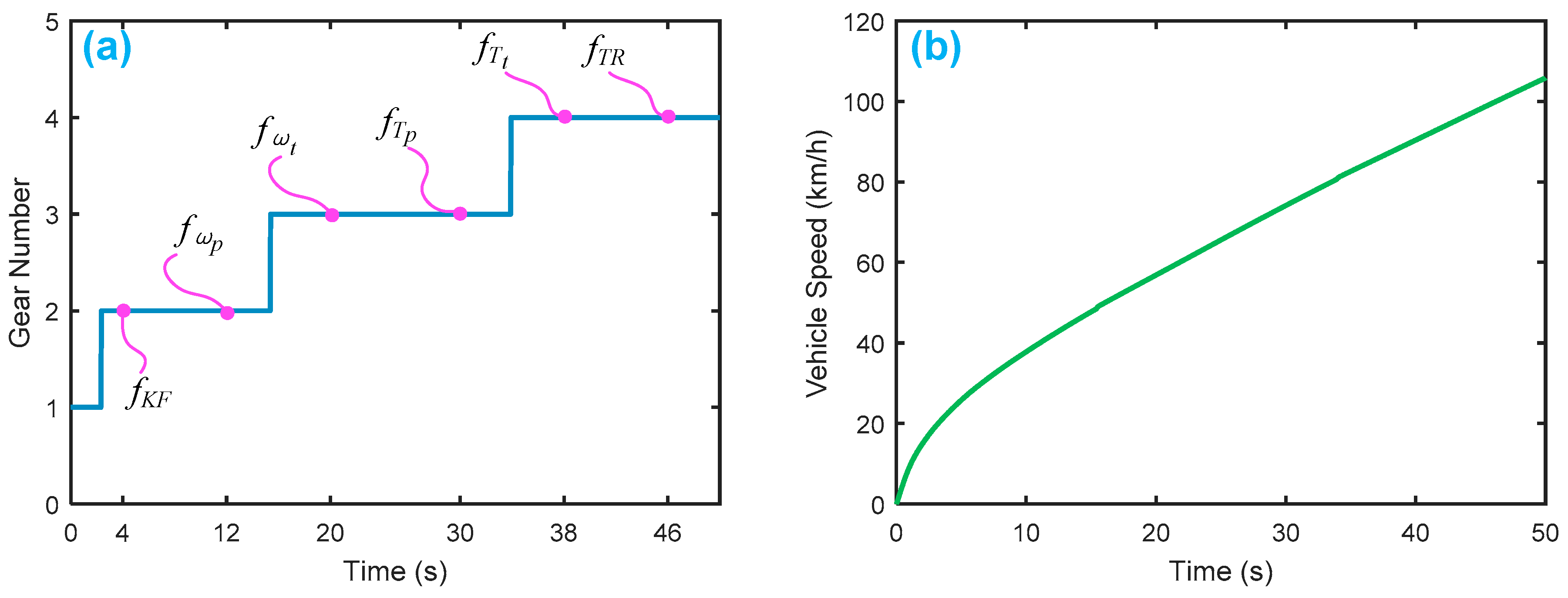
| Fault | Type | Signal | Time Span |
|---|---|---|---|
| Gain (1.5) |  | 4–6 s | |
| Bias (−150) |  | 12–14 s | |
| Bias (+200) |  | 20–22 s | |
| Gain (2) |  | 30–32 s | |
| Gain (0.5) |  | 38–40 s | |
| Gain (0) |  | 46–48 s |
| - | ||||||
|---|---|---|---|---|---|---|
| × | ● | ● | ● | ● | ● | |
| ● | × | ● | ● | ● | ● | |
| ● | ● | × | ● | ● | ● | |
| ● | ● | ● | × | ● | ● | |
| ● | ● | ● | ● | × | × |
| Fault | Type | Signal | Time Span |
|---|---|---|---|
| Bias (+500) |  | 1–1.2 s | |
| Bias (−1000) |  | 2–2.2 s | |
| Gain (0) |  | 3–3.2 s | |
| Gain (10) |  | 4–4.2 s |
| ● | ● | ● | ● | |
| × | ● | ● | ● | |
| ● | × | ● | ● | |
| ● | ● | × | ● | |
| ● | ● | ● | × |
© 2018 by the authors. Licensee MDPI, Basel, Switzerland. This article is an open access article distributed under the terms and conditions of the Creative Commons Attribution (CC BY) license (http://creativecommons.org/licenses/by/4.0/).
Share and Cite
Chen, Q.; Wang, J.; Ahmed, Q. Design and Evaluation of a Structural Analysis-Based Fault Detection and Identification Scheme for a Hydraulic Torque Converter. Sensors 2018, 18, 4103. https://doi.org/10.3390/s18124103
Chen Q, Wang J, Ahmed Q. Design and Evaluation of a Structural Analysis-Based Fault Detection and Identification Scheme for a Hydraulic Torque Converter. Sensors. 2018; 18(12):4103. https://doi.org/10.3390/s18124103
Chicago/Turabian StyleChen, Qi, Jincheng Wang, and Qadeer Ahmed. 2018. "Design and Evaluation of a Structural Analysis-Based Fault Detection and Identification Scheme for a Hydraulic Torque Converter" Sensors 18, no. 12: 4103. https://doi.org/10.3390/s18124103
APA StyleChen, Q., Wang, J., & Ahmed, Q. (2018). Design and Evaluation of a Structural Analysis-Based Fault Detection and Identification Scheme for a Hydraulic Torque Converter. Sensors, 18(12), 4103. https://doi.org/10.3390/s18124103