Measuring Linewidth Enhancement Factor by Relaxation Oscillation Frequency in a Laser with Optical Feedback


Abstract
1. Introduction
2. Measurement Theory
3. Simulation Test
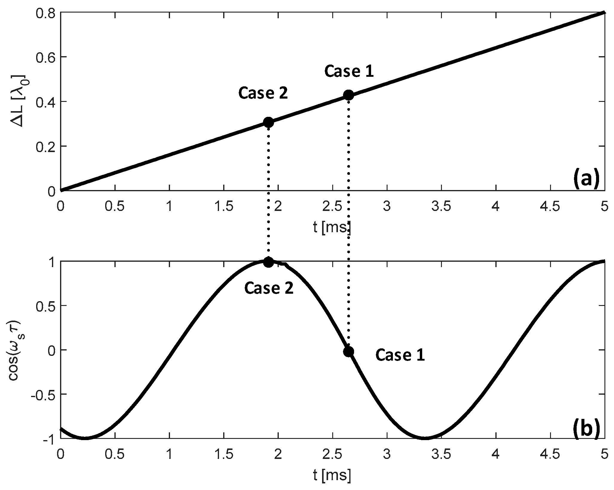
- Starting from , increase the cavity length and set it with 6 different locations.
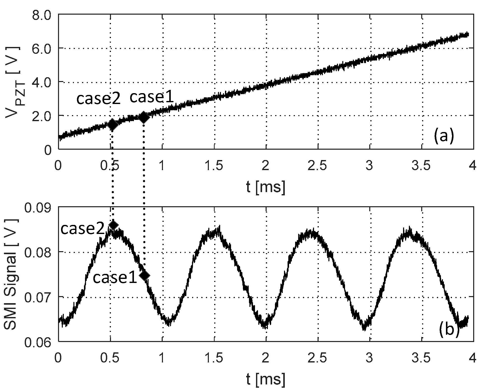
- At each location, apply a micro displacement onto the external cavity with 0.8 wavelength shown on Figure 2a. Correspondingly, we can use the SMI model described in by Equations (4) and (7) to plot an SMI signal shown in Figure 2b, on which we can locate the accurate locations for case 1 and case 2.
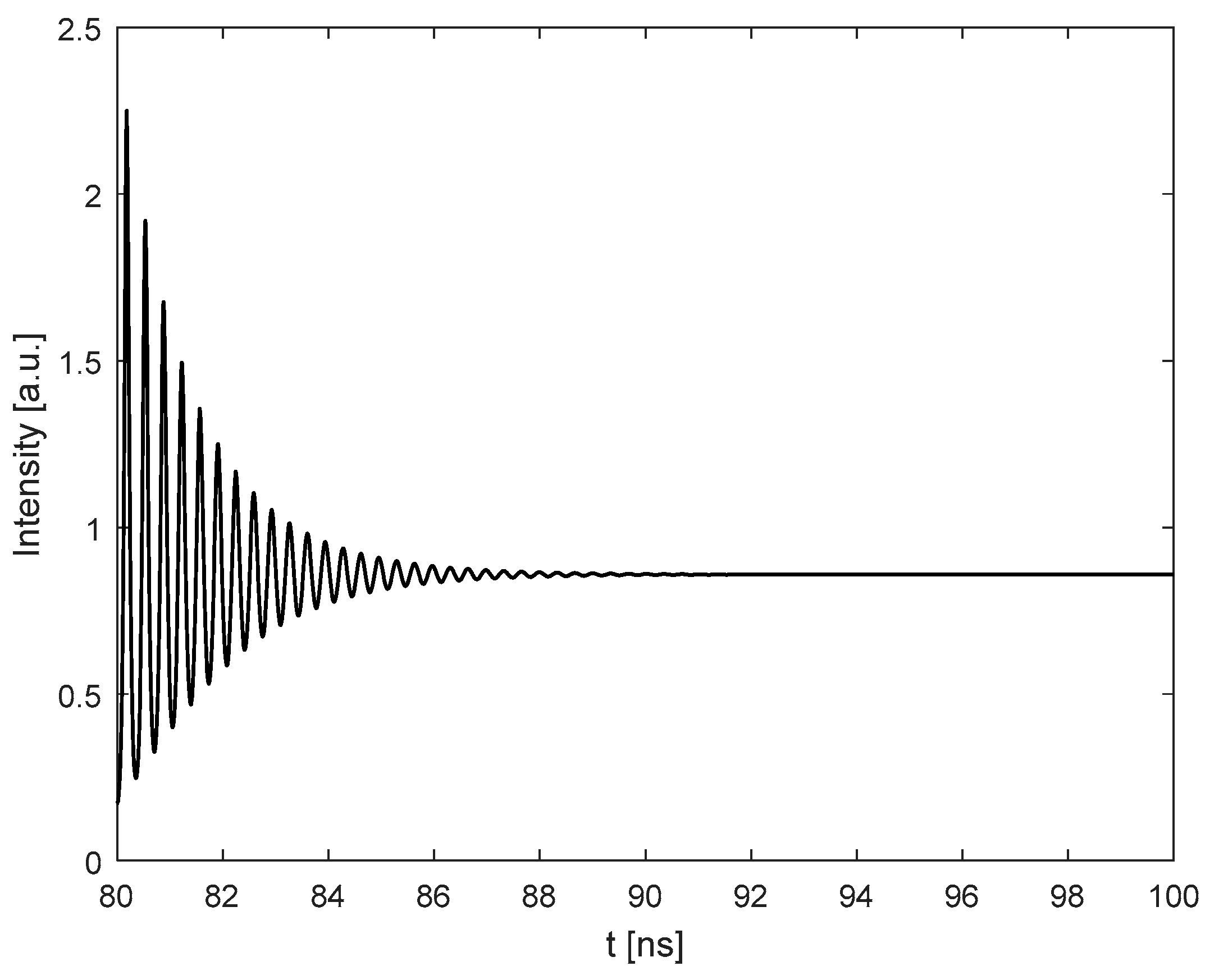
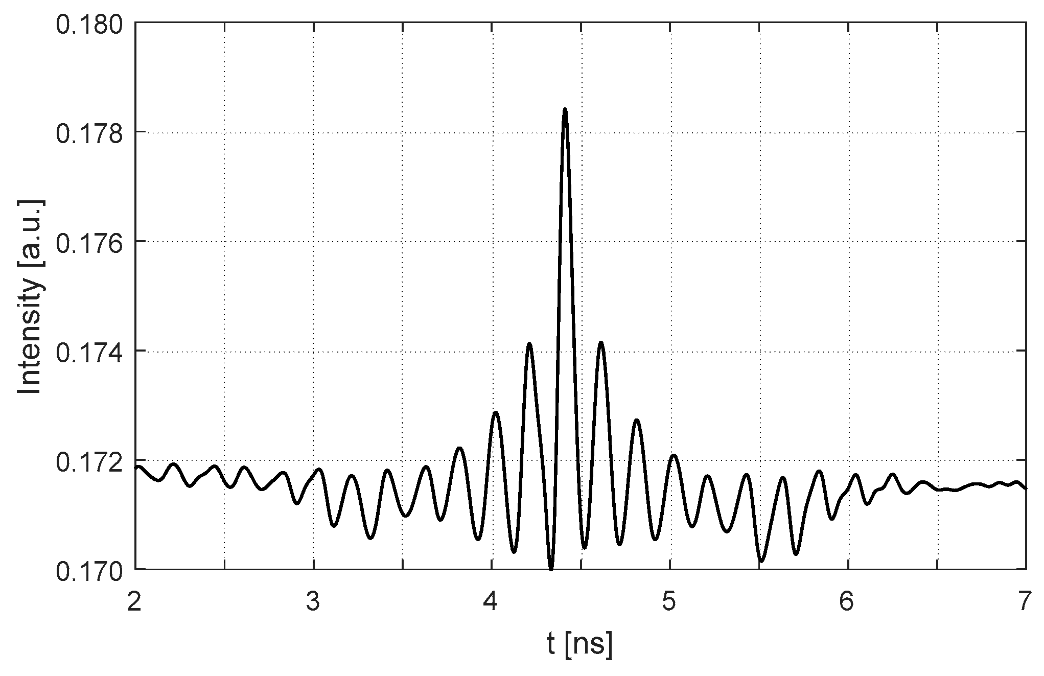
- With the results obtained at step 2 for case 1 and case 2, generate the corresponding laser intensity by numerically solving the L-K equations. E.g., the laser transient waveform for case 1 shown in Figure 3, from which, the RO frequency can be obtained.
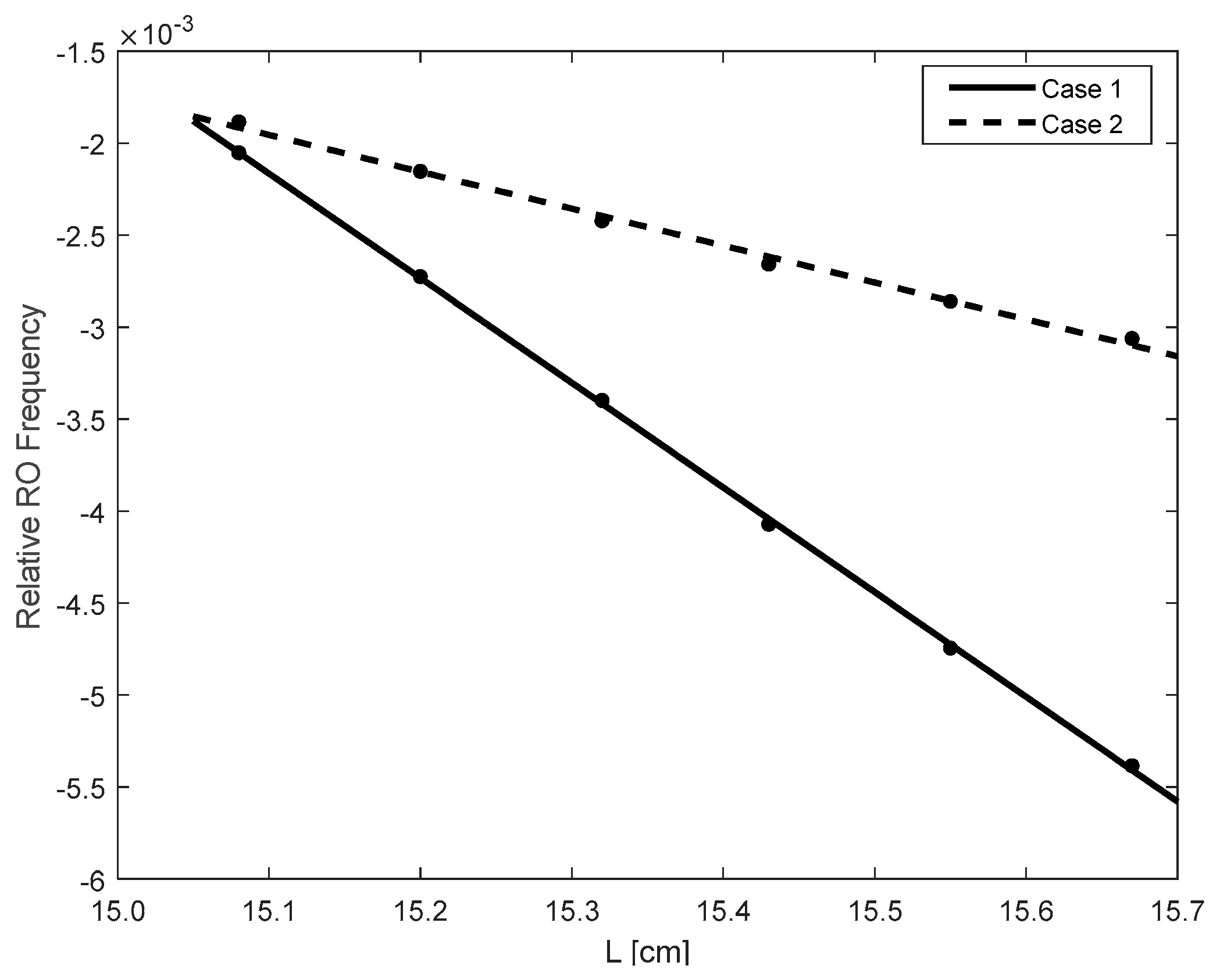
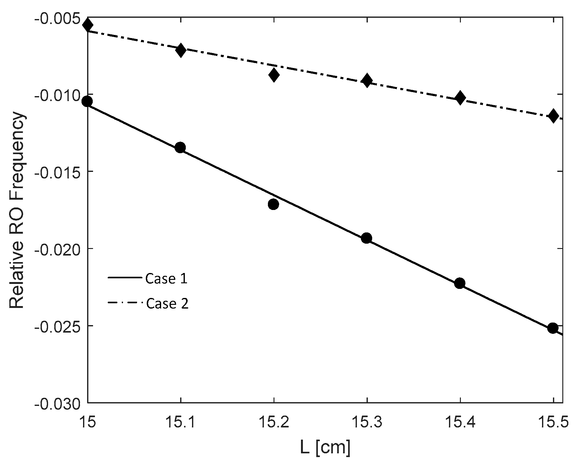
- Repeat steps 2 and 3 for the 6 different locations, we get 6 RO frequencies for each case, denoted by and , i = 1,2, … 6. The relationship between the relative RO frequency () and the cavity length L for the two cases are depicted on Figure 4. Note that the gradient can be determined by only 2 points. In order to reduce the measured error, we prefer to use more than 2 points, e.g., 6 points to do line fitting to get the gradients at each case. From the gradients of these two fitting lines, can be calculated by using Equation (15).
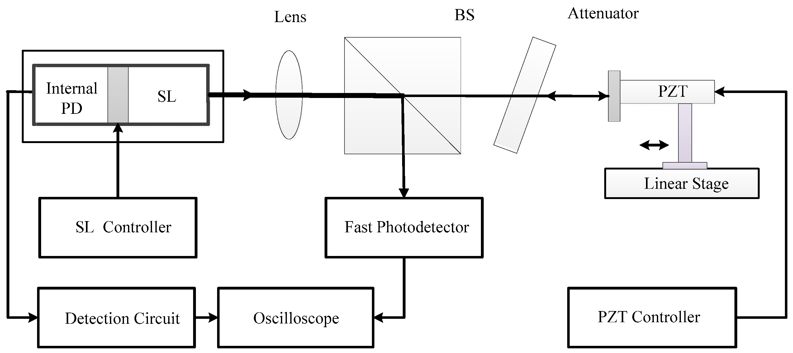
4. Experiments
5. Conclusions
Author Contributions
Funding
Conflicts of Interest
References
- Henry, C. Theory of the linewidth of semiconductor lasers. IEEE J. Quantum Electron. 1982, 18, 259–264. [Google Scholar] [CrossRef]
- Osinski, M.; Buus, J. Linewidth broadening factor in semiconductor lasers-An overview. IEEE J. Quantum Electron. 1987, 23, 9–29. [Google Scholar] [CrossRef]
- Fordell, T.; Lindberg, A.M. Experiments on the Linewidth-Enhancement Factor of a Vertical-Cavity Surface-Emitting Laser. IEEE J. Quantum Electron. 2007, 43, 6–15. [Google Scholar] [CrossRef]
- Henning, I.D.; Collins, J.V. Measurements of the semiconductor laser linewidth broadening factor. Electron. Lett. 1983, 19, 927–929. [Google Scholar] [CrossRef]
- Kowalski, B.; Debeau, J.; Boittin, R. A simple and novel method for measuring the chirp parameter of an intensity modulated light source. IEEE Photonics Technol. Lett. 1999, 11, 700–702. [Google Scholar] [CrossRef]
- Liu, G.; Jin, X.; Chuang, S.L. Measurement of linewidth enhancement factor of semiconductor lasers using an injection-locking technique. IEEE Photonics Technol. Lett. 2001, 13, 430–432. [Google Scholar] [CrossRef]
- Yu, Y.; Giuliani, G.; Donati, S. Measurement of the linewidth enhancement factor of semiconductor lasers based on the optical feedback self-mixing effect. IEEE Photonics Technol. Lett. 2004, 16, 990–992. [Google Scholar] [CrossRef]
- Xi, J.; Yu, Y.; Chicharo, J.; Bosch, T. Estimating the parameters of semiconductor lasers based on weak optical feedback self-mixing interferometry. IEEE J. Quantum Electron. 2005, 41, 1058–1064. [Google Scholar]
- Yu, Y.; Xi, J.; Chicharo, J.; Bosch, T. Toward Automatic Measurement of the Linewidth-Enhancement Factor Using Optical Feedback Self-Mixing Interferometry With Weak Optical Feedback. IEEE J. Quantum Electron. 2007, 43, 527–534. [Google Scholar] [CrossRef]
- Yu, Y.; Xi, J. Influence of external optical feedback on the alpha factor of semiconductor lasers. Opt. Lett. 2013, 38, 1781–1783. [Google Scholar] [CrossRef] [PubMed]
- Norgia, M.; Donati, S.; D’Alessandro, D. Interferometric measurements of displacement on a diffusing target by a speckle tracking technique. IEEE J. Quantum Electron. 2001, 37, 800–806. [Google Scholar] [CrossRef]
- Zabit, U.; Bony, F.; Bosch, T.; Rakic, A.D. A Self-Mixing Displacement Sensor with Fringe-Loss Compensation for Harmonic Vibrations. IEEE Photonics Technol. Lett. 2010, 22, 410–412. [Google Scholar] [CrossRef]
- Zhang, S.; Zhang, S.; Tan, Y.; Sun, L. A microchip laser source with stable intensity and frequency used for self-mixing interferometry. Rev. Sci. Instrum. 2016, 87, 053114. [Google Scholar] [CrossRef] [PubMed]
- Norgia, M.; Melchionni, D.; Pesatori, A. Self-mixing instrument for simultaneous distance and speed measurement. Opt. Lasers Eng. 2017, 99, 31–38. [Google Scholar] [CrossRef]
- Bes, C.; Plantier, G.; Bosch, T. Displacement measurements using a self-mixing laser diode under moderate feedback. IEEE Trans. Instrum. Meas. 2006, 55, 1101–1105. [Google Scholar] [CrossRef]
- Taimre, T.; Nikolić, M.; Bertling, K.; Lim, Y.L.; Bosch, T.; Rakić, A.D. Laser feedback interferometry: A tutorial on the self-mixing effect for coherent sensing. Adv. Opt. Photonics 2015, 7, 570–631. [Google Scholar] [CrossRef]
- Guo, D.; Wang, M.; Tan, S. Self-mixing interferometer based on sinusoidal phase modulating technique. Opt. Express 2005, 13, 1537–1543. [Google Scholar] [CrossRef] [PubMed]
- Wei, L.; Xi, J.; Yu, Y.; Chicharo, J.F. Linewidth enhancement factor measurement based on optical feedback self-mixing effect: A genetic algorithm approach. J. Opt. A Pure Appl. Opt. 2009, 11, 045505. [Google Scholar] [CrossRef]
- Fan, Y.; Yu, Y.; Xi, J.; Chicharo, J.F. Improving the measurement performance for a self-mixing interferometry-based displacement sensing system. Appl. Opt. 2011, 50, 5064–5072. [Google Scholar] [CrossRef] [PubMed]
- Donati, S.; Giuliani, G.; Merlo, S. Laser diode feedback interferometer for measurement of displacements without ambiguity. IEEE J. Quantum Electron. 1995, 31, 113–119. [Google Scholar] [CrossRef]
- Lacot, E.; Day, R.; Stoeckel, F. Coherent laser detection by frequency-shifted optical feedback. Phys. Rev. A 2001, 64, 043815. [Google Scholar] [CrossRef]
- Liu, B.; Yu, Y.; Xi, J.; Guo, Q.; Tong, J.; Lewis, R.A. Displacement sensing using the relaxation oscillation frequency of a laser diode with optical feedback. Appl. Opt. 2017, 56, 6962–6966. [Google Scholar] [CrossRef] [PubMed]
- Lang, R.; Kobayashi, K. External optical feedback effects on semiconductor injection laser properties. IEEE J. Quantum Electron. 1980, 16, 347–355. [Google Scholar] [CrossRef]
- Uchida, A. Optical Communication with Chaotic Lasers: Applications of Nonlinear Dynamics and Synchronization; John Wiley & Sons: Hoboken, NJ, USA, 2012; pp. 206–208. [Google Scholar]
- Kane, D.M.; Toomey, J.P. Precision Threshold Current Measurement for Semiconductor Lasers Based on Relaxation Oscillation Frequency. J. Lightwave Technol. 2009, 27, 2949–2952. [Google Scholar] [CrossRef]


| Symbol | Physical Meaning | Value |
|---|---|---|
| Feedback strength | ||
| External cavity round trip time,, where L is external cavity length, c is speed of light | ||
| Angular frequency of solitary laser | ||
| Line-width enhancement factor | ||
| Injection current density | ||
| Threshold injection current density | ||
| Internal cavity round-trip time | ||
| Photon life time | ||
| Carrier life time | ||
| Modal gain coefficient | ||
| Carrier density at transparency | ||
| Nonlinear gain compression coefficient | ||
| Confinement factor |
| 0.50 | 0.52 | 3.8% |
| 1.00 | 1.01 | 0.6% |
| 2.00 | 2.04 | 1.9% |
| 3.00 | 2.94 | 2.0% |
| 4.00 | 3.81 | 4.8% |
| 5.00 | 4.75 | 5.0% |
| 0.50 | 0.51 | 2.4% |
| 1.00 | 1.04 | 4.2% |
| 2.00 | 2.05 | 2.7% |
| 3.00 | 3.08 | 2.7% |
| 4.00 | 4.01 | 0.2% |
| 5.00 | 4.82 | 3.7% |
| L (cm) | 15.0 | 15.1 | 15.2 | 15.3 | 15.4 | 15.5 |
| 4.631 | 4.645 | 4.659 | 4.669 | 4.687 | 4.701 | |
| 4.697 | 4.702 | 4.708 | 4.709 | 4.717 | 4.725 | |
| 4.751 | ||||||
| , , . | ||||||
© 2018 by the authors. Licensee MDPI, Basel, Switzerland. This article is an open access article distributed under the terms and conditions of the Creative Commons Attribution (CC BY) license (http://creativecommons.org/licenses/by/4.0/).
Share and Cite
Ruan, Y.; Liu, B.; Yu, Y.; Xi, J.; Guo, Q.; Tong, J. Measuring Linewidth Enhancement Factor by Relaxation Oscillation Frequency in a Laser with Optical Feedback. Sensors 2018, 18, 4004. https://doi.org/10.3390/s18114004
Ruan Y, Liu B, Yu Y, Xi J, Guo Q, Tong J. Measuring Linewidth Enhancement Factor by Relaxation Oscillation Frequency in a Laser with Optical Feedback. Sensors. 2018; 18(11):4004. https://doi.org/10.3390/s18114004
Chicago/Turabian StyleRuan, Yuxi, Bin Liu, Yanguang Yu, Jiangtao Xi, Qinghua Guo, and Jun Tong. 2018. "Measuring Linewidth Enhancement Factor by Relaxation Oscillation Frequency in a Laser with Optical Feedback" Sensors 18, no. 11: 4004. https://doi.org/10.3390/s18114004
APA StyleRuan, Y., Liu, B., Yu, Y., Xi, J., Guo, Q., & Tong, J. (2018). Measuring Linewidth Enhancement Factor by Relaxation Oscillation Frequency in a Laser with Optical Feedback. Sensors, 18(11), 4004. https://doi.org/10.3390/s18114004