Multi-Year Mapping of Major Crop Yields in an Irrigation District from High Spatial and Temporal Resolution Vegetation Index


Abstract
1. Introduction
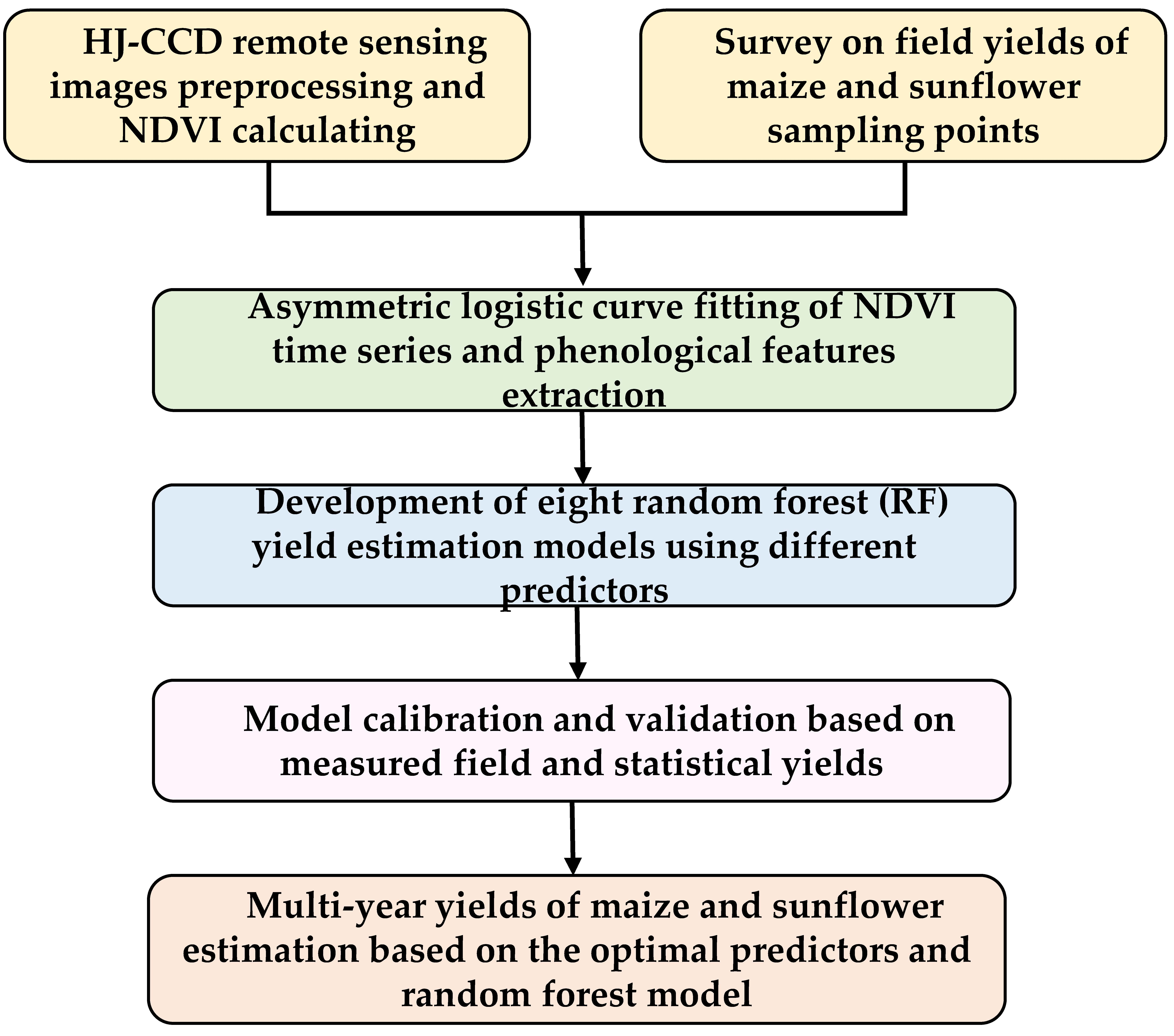
2. Study Area
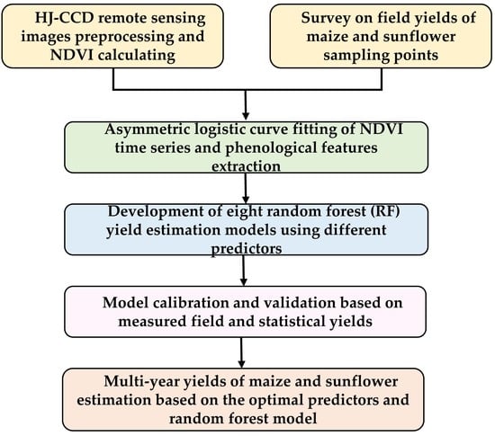
3. Data and Method
3.1. Data Sources
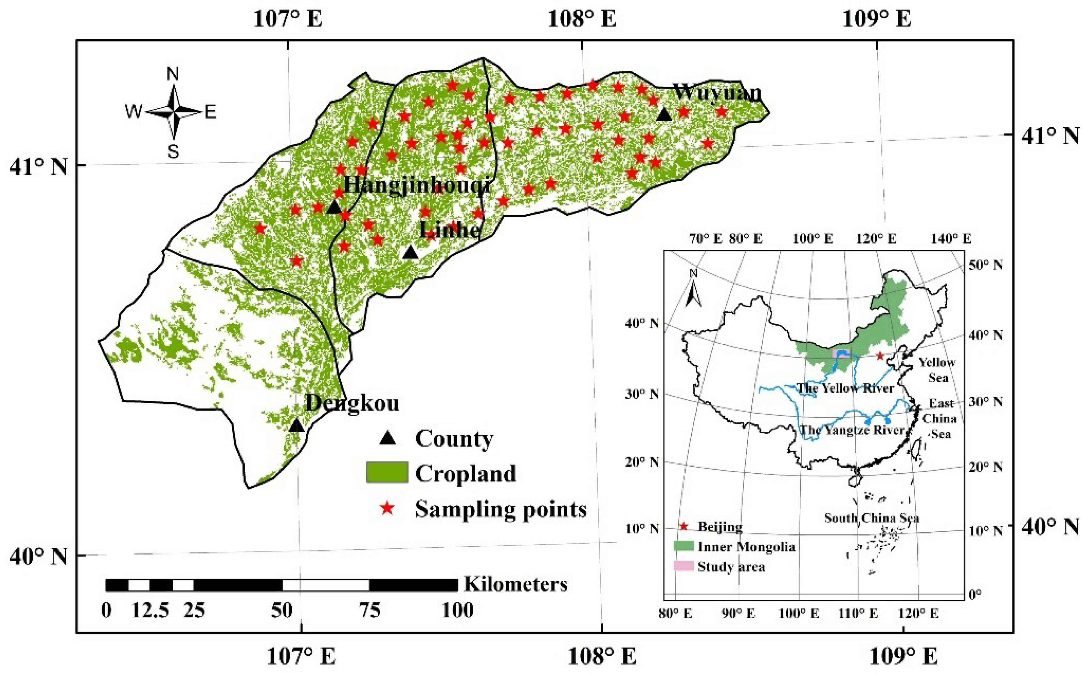
3.2. Data Processing and Determination of Model Input
3.3. Random Forest Regression Algorithm
3.4. Model Calibration and Validation
4. Results and Discussion
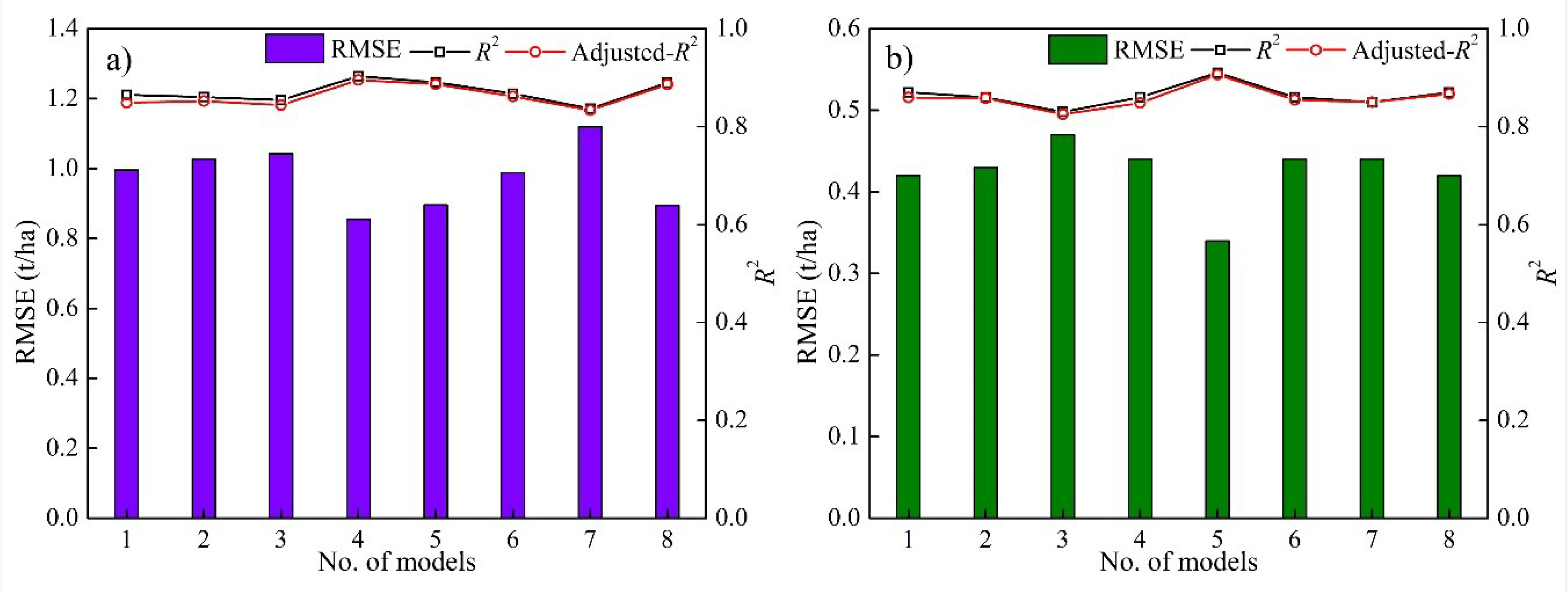
4.1. Model Calibration with Field Measured Yields at Pixel Level
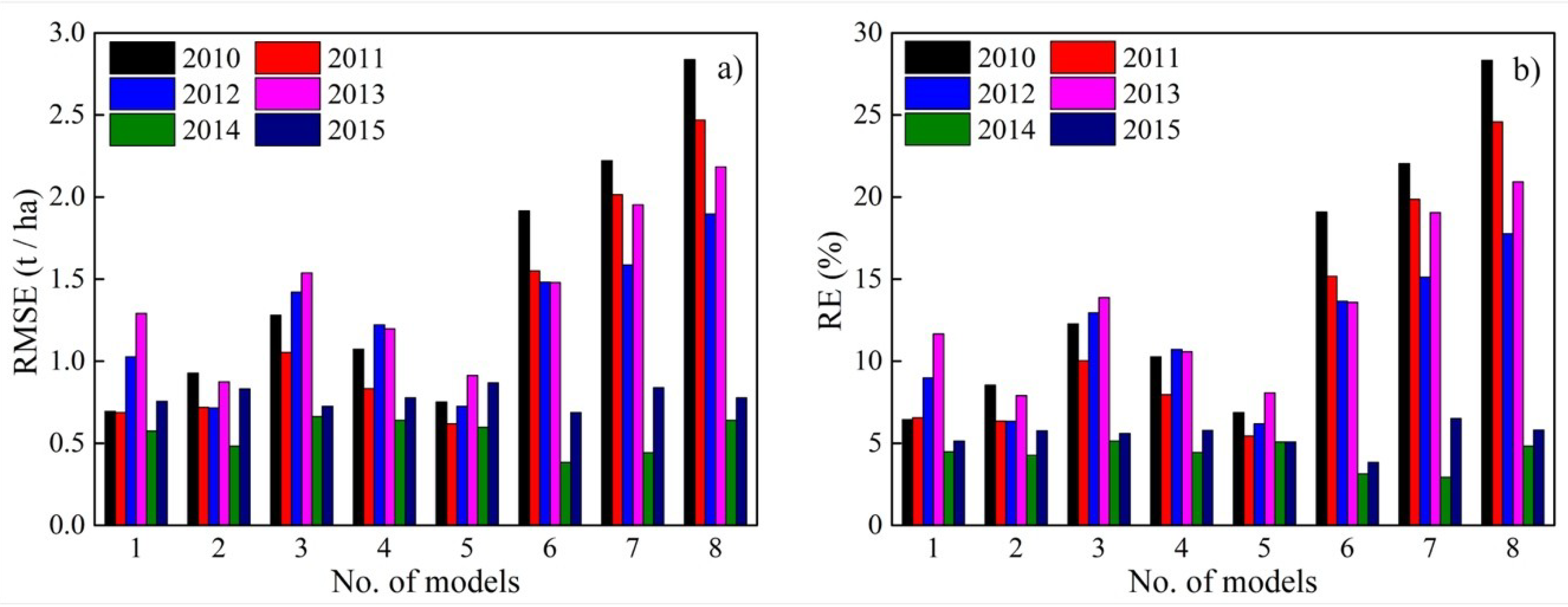
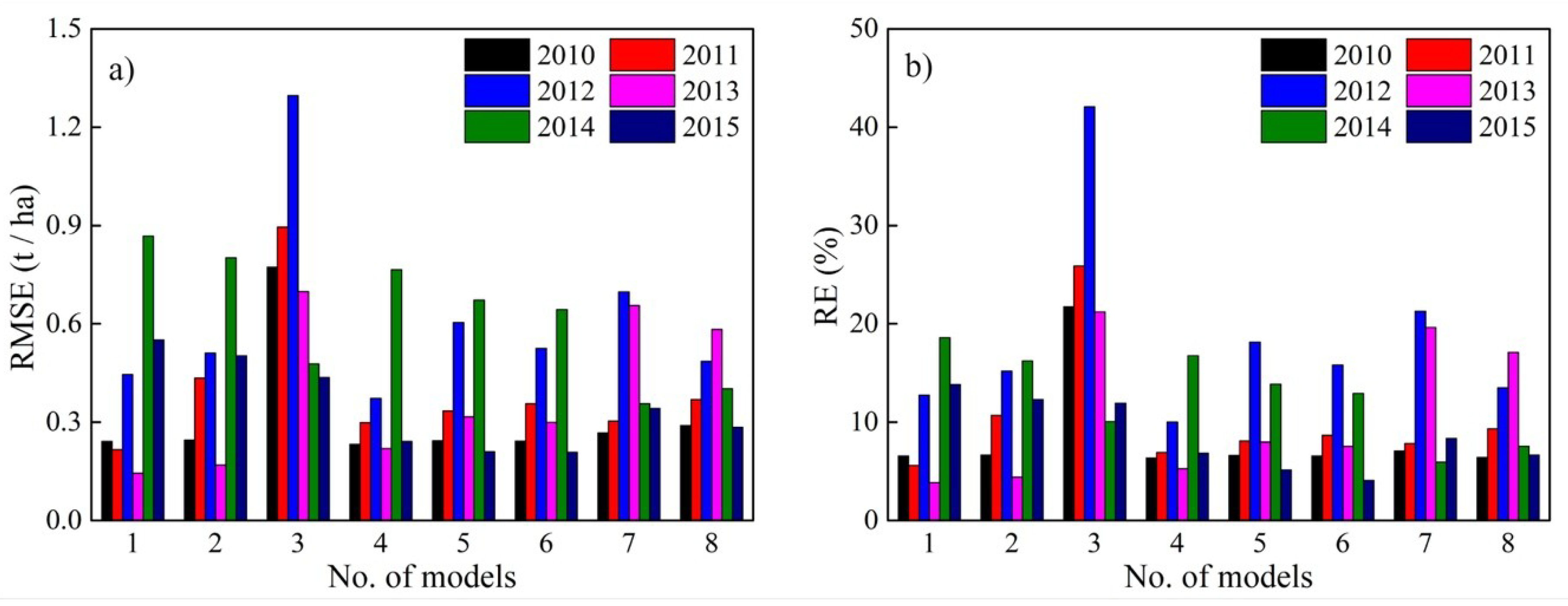
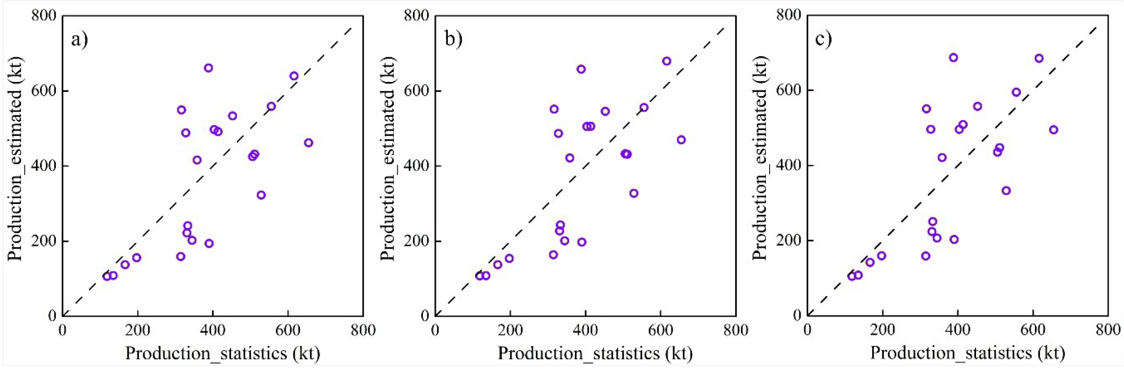
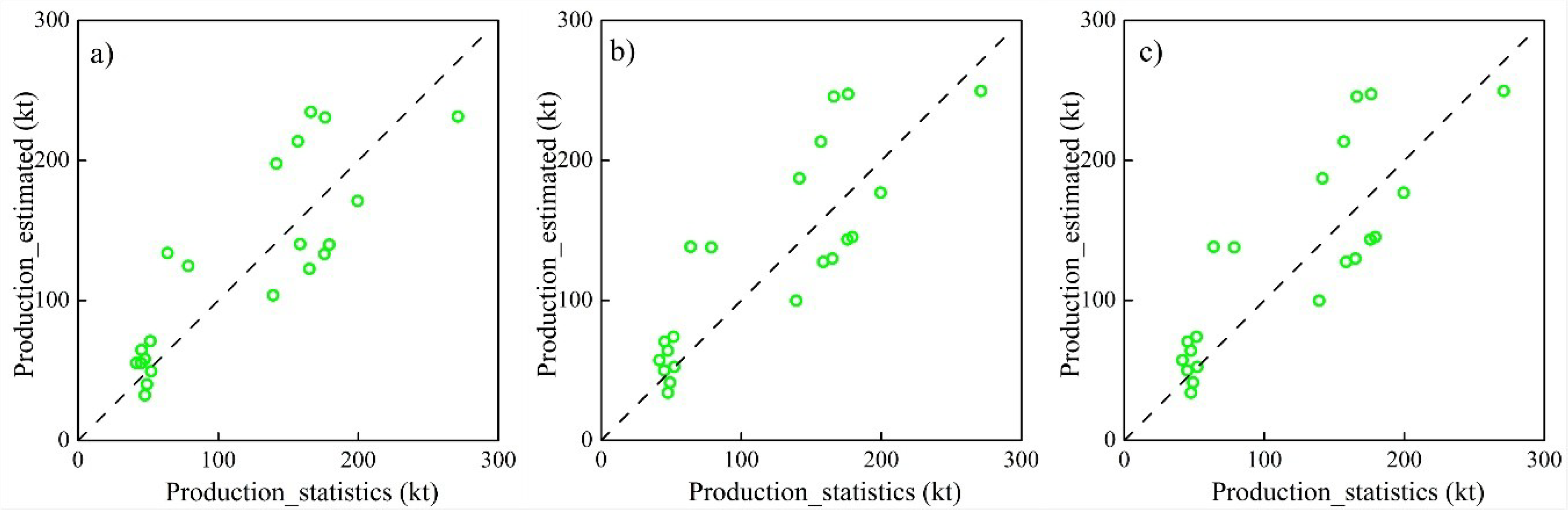
4.2. Model Validation with Statistical Yield and Production at the County Level
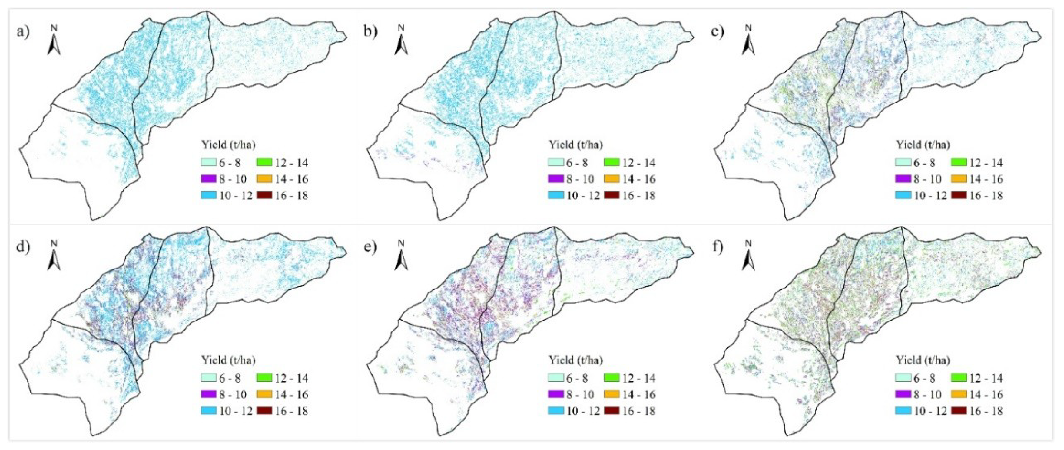
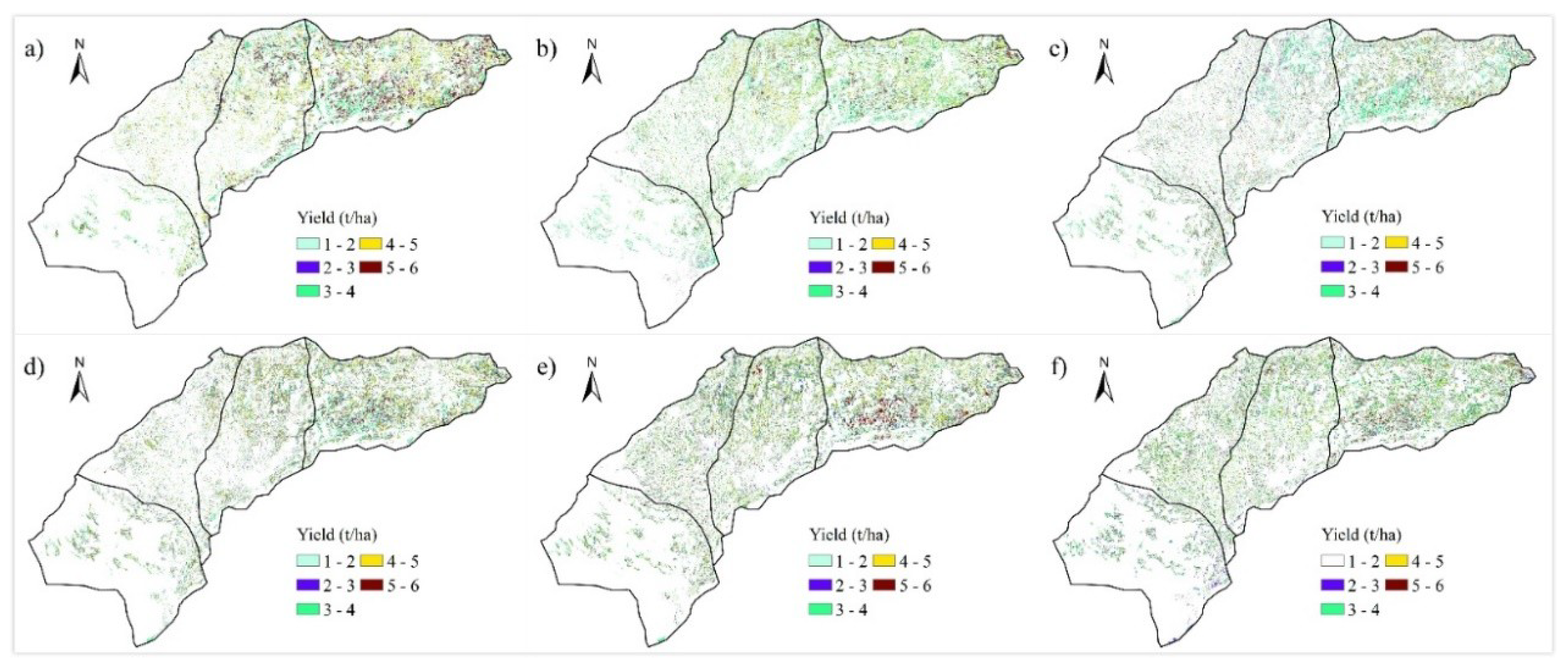
4.3. Spatial and Temporal Distribution of Crop Yields
5. Conclusions
- (1)
- The RF model could accurately estimate annual regional crop yields, with the multi-year average values of root-mean-square error and the relative error of 0.75 t/ha and 6.1% for maize, and 0.40 t/ha and 10.1% for sunflower, respectively.
- (2)
- Among eight models, the optimal model for maize was NDVI series from the 120th day to the 210th day with 10 days’ interval, while the optimal model for sunflower was the combination of NDVI indexes and phenological characteristics.
- (3)
- The yields of maize and sunflower could be estimated fairly well with NDVI series 50 days before crop harvest, which implicated the possibility of crop yield forecast before harvest.
Author Contributions
Funding
Acknowledgments
Conflicts of Interest
References
- The State of Food Security and Nutrition in the World (SOFI) Report. Available online: https://www.wfp.org/content/2017-state-food-security-and-nutrition-world-sofi-report (accessed on 20 August 2018).
- Hutchinson, C.F. Uses of satellite data for famine early warning in sub-Saharan Africa. Int. J. Remote Sens. 1991, 12, 1405–1421. [Google Scholar] [CrossRef]
- Kowalik, W.; Dabrowska, Z.K.; Meroni, M.; Raczka, T.U.; de Wit, A. Yield estimation using SPOT-VEGETATION products: A case study of wheat in European countries. Int. J. Appl. Earth Obs. Geoinf. 2014, 32, 228–239. [Google Scholar] [CrossRef]
- Noureldin, N.A.; Aboelghar, M.A.; Saudy, H.S.; Ali, A.M. Rice yield forecasting models using satellite imagery in Egypt. Egypt. J. Remote Sens. Space Sci. 2013, 16, 125–131. [Google Scholar] [CrossRef]
- Cunha, M.; Marçal, A.R.S.; Silva, L. Very early prediction of wine yield based on satellite data from VEGETATION. Int. J. Remote Sens. 2010, 31, 3125–3142. [Google Scholar] [CrossRef]
- Zhang, X.; Zhang, Q. Monitoring interannual variation in global crop yield using long-term AVHRR and MODIS observations. ISPRS J. Photogramm. Remote Sens. 2016, 114, 191–205. [Google Scholar] [CrossRef]
- Shao, Y.; Campbell, J.B.; Taff, G.N.; Zheng, B. An analysis of cropland mask choice and ancillary data for annual corn yield forecasting using MODIS data. Int. J. Appl. Earth Obs. Geoinf. 2015, 38, 78–87. [Google Scholar] [CrossRef]
- Johnson, D.M. An assessment of pre- and within-season remotely sensed variables for forecasting corn and soybean yields in the United States. Remote Sens. Environ. 2014, 141, 116–128. [Google Scholar] [CrossRef]
- Skakun, S.; Franch, B.; Vermote, E.; Roger, J.; Becker, R.I.; Justice, C.; Kussul, N. Early season large-area winter crop mapping using MODIS NDVI data, growing degree days information and a Gaussian mixture model. Remote Sens. Environ. 2017, 195, 244–258. [Google Scholar] [CrossRef]
- Zhong, L.; Hu, L.; Yu, L.; Gong, P.; Biging, G.S. Automated mapping of soybean and corn using phenology. ISPRS J. Photogramm. Remote Sens. 2016, 119, 151–164. [Google Scholar] [CrossRef]
- Fieuzal, R.; Marais, S.C.; Baup, F. Estimation of corn yield using multi-temporal optical and radar satellite data and artificial neural networks. Int. J. Appl. Earth Obs. Geoinf. 2017, 57, 14–23. [Google Scholar] [CrossRef]
- Mulianga, B.; Bégué, A.; Simoes, M.; Todoroff, P. Forecasting regional sugarcane yield based on time integral and spatial aggregation of MODIS NDVI. Remote Sens. 2013, 5, 2184–2199. [Google Scholar] [CrossRef]
- Son, N.T.; Chen, C.F.; Chen, C.R.; Minh, V.Q.; Trung, N.H. A comparative analysis of multitemporal MODIS EVI and NDVI data for large-scale rice yield estimation. Agric. For. Meteorol. 2014, 197, 52–64. [Google Scholar] [CrossRef]
- Balaghi, R.; Tychon, B.; Eerens, H.; Jlibene, M. Empirical regression models using NDVI, rainfall and temperature data for the early prediction of wheat grain yields in Morocco. Int. J. Appl. Earth Obs. Geoinf. 2008, 10, 438–452. [Google Scholar] [CrossRef]
- Bolton, D.K.; Friedl, M.A. Forecasting crop yield using remotely sensed vegetation indices and crop phenology metrics. Agric. For. Meteorol. 2013, 173, 74–84. [Google Scholar] [CrossRef]
- Johnson, M.D.; Hsieh, W.W.; Cannon, A.J.; Davidson, A.; Bédard, F. Crop yield forecasting on the Canadian Prairies by remotely sensed vegetation indices and machine learning methods. Agric. For. Meteorol. 2016, 218–219, 74–84. [Google Scholar] [CrossRef]
- Fernandez-Ordoñez, Y.M.; Soria-Ruiz, J. Maize crop yield estimation with remote sensing and empirical models. In Proceedings of the IEEE International Geoscience and Remote Sensing Symposium, Fort Worth, TX, USA, 23–28 July 2017; IEEE: Piscataway, NJ, USA, 2017. [Google Scholar]
- Kuri, F.; Murwira, A.; Murwira, K.S.; Masocha, M. Predicting maize yield in Zimbabwe using dry dekads derived from remotely sensed Vegetation Condition Index. Int. J. Appl. Earth Obs. Geoinf. 2014, 33, 39–46. [Google Scholar] [CrossRef]
- Ban, H.; Kim, K.; Park, N.; Lee, B. Using MODIS Data to Predict Regional Corn Yields. Remote Sens. 2017, 9, 16. [Google Scholar] [CrossRef]
- Holzman, M.E.; Rivas, R.; Piccolo, M.C. Estimating soil moisture and the relationship with crop yield using surface temperature and vegetation index. Int. J. Appl. Earth Obs. Geoinf. 2014, 28, 181–192. [Google Scholar] [CrossRef]
- De Wit, A.; Duveiller, G.; Defourny, P. Estimating regional winter wheat yield with WOFOST through the assimilation of green area index retrieved from MODIS observations. Agric. For. Meteorol. 2012, 164, 39–52. [Google Scholar] [CrossRef]
- Jin, X.; Li, Z.; Yang, G.; Yang, H.; Feng, H.; Xu, X.; Wang, J.; Li, X.; Luo, J. Winter wheat yield estimation based on multi-source medium resolution optical and radar imaging data and the AquaCrop model using the particle swarm optimization algorithm. ISPRS J. Photogramm Remote Sens. 2017, 126, 24–37. [Google Scholar] [CrossRef]
- Xie, Y.; Wang, P.; Bai, X.; Khan, J.; Zhang, S.; Li, L.; Wang, L. Assimilation of the leaf area index and vegetation temperature condition index for winter wheat yield estimation using Landsat imagery and the CERES-Wheat model. Agric. For. Meteorol. 2017, 246, 194–206. [Google Scholar] [CrossRef]
- Huang, J.; Ma, H.; Su, W.; Zhang, X.; Huang, Y.; Fan, J.; Wu, W. Jointly assimilating MODIS LAI and ET products into the SWAP model for winter wheat yield estimation. IEEE J. Sel. Top. Appl. Earth Obs. Remote Sens. 2015, 8, 4060–4071. [Google Scholar] [CrossRef]
- Cheng, Z.; Meng, J.; Qiao, Y.; Wang, Y.; Dong, W.; Han, Y. Preliminary study of soil available nutrient simulation using a modified WOFOST model and time-series remote sensing observations. Remote Sens. 2018, 10, 64. [Google Scholar] [CrossRef]
- Silvestro, P.; Pignatti, S.; Pascucci, S.; Yang, H.; Li, Z.; Yang, G.; Huang, W.; Casa, R. Estimating Wheat Yield in China at the Field and District Scale from the Assimilation of Satellite Data into the Aquacrop and Simple Algorithm for Yield (SAFY) Models. Remote Sens. 2017, 9, 509. [Google Scholar] [CrossRef]
- Zhao, Y.; Chen, S.; Shen, S. Assimilating remote sensing information with crop model using Ensemble Kalman Filter for improving LAI monitoring and yield estimation. Ecol. Model. 2013, 270, 30–42. [Google Scholar] [CrossRef]
- Ma, G.; Huang, J.; Wu, W.; Fan, J.; Zou, J.; Wu, S. Assimilation of MODIS-LAI into the WOFOST model for forecasting regional winter wheat yield. Math. Comput. Model. 2013, 58, 634–643. [Google Scholar] [CrossRef]
- Ma, Y.P.; Wang, S.L.; Zhang, L.; Hou, Y.Y.; Zhuang, L.W.; He, Y.B.; Wang, F.T. Monitoring winter wheat growth in North China by combining a crop model and remote sensing data. Int. J. Appl. Earth Obs. Geoinf. 2008, 10, 426–437. [Google Scholar] [CrossRef]
- Peng, D.; Huang, J.; Li, C.; Liu, L.; Huang, W.; Wang, F.; Yang, X. Modelling paddy rice yield using MODIS data. Agric. For. Meteorol. 2014, 184, 107–116. [Google Scholar] [CrossRef]
- Bandaru, V.; West, T.O.; Ricciuto, D.M.; César, I.R. Estimating crop net primary production using national inventory data and MODIS-derived parameters. ISPRS J. Photogramm. Remote Sens. 2013, 80, 61–71. [Google Scholar] [CrossRef]
- Lobell, D.B.; Asner, G.P.; Ortiz-Monasterio, J.I.; Benning, T.L. Remote sensing of regional crop production in the Yaqui Valley, Mexico: Estimates and uncertainties. Agric. Ecosyst. Environ. 2003, 94, 205–220. [Google Scholar] [CrossRef]
- Xin, Q.; Gong, P.; Yu, C.; Yu, L.; Broich, M.; Suyker, A.; Myneni, R. A production efficiency model-based method for satellite estimates of corn and soybean yields in the Midwestern US. Remote Sens. 2013, 5, 5926–5943. [Google Scholar] [CrossRef]
- Shao, Y.; Lunetta, R.S. Comparison of support vector machine, neural network, and CART algorithms for the land-cover classification using limited training data points. ISPRS J. Photogramm. Remote Sens. 2012, 70, 78–87. [Google Scholar] [CrossRef]
- Shao, Y.; Taff, G.N.; Ren, J.; Campbell, J.B. Characterizing major agricultural land change trends in the Western Corn Belt. ISPRS J. Photogramm. Remote Sens. 2016, 122, 116–125. [Google Scholar] [CrossRef]
- Ng, W.; Meroni, M.; Immitzer, M.; Böck, S.; Leonardi, U.; Rembold, F.; Gadain, H.; Atzberger, C. Mapping Prosopis spp. with Landsat 8 data in arid environments: Evaluating effectiveness of different methods and temporal imagery selection for Hargeisa, Somaliland. Int. J. Appl. Earth Obs. Geoinf. 2016, 53, 76–89. [Google Scholar] [CrossRef]
- Bose, P.; Kasabov, N.K.; Bruzzone, L.; Hartono, R.N. Spiking Neural Networks for Crop Yield Estimation Based on Spatiotemporal Analysis of Image Time Series. IEEE Trans. Geosci. Remote Sens. 2016, 54, 6563–6573. [Google Scholar] [CrossRef]
- Fortin, J.G.; Anctil, F.; Parent, L.; Bolinder, M.A. Site-specific early season potato yield forecast by neural network in Eastern Canada. Precis. Agric. 2011, 12, 905–923. [Google Scholar] [CrossRef]
- Villanueva, B.M.; Salenga, M.L.M. Bitter Melon Crop Yield Prediction using Machine Learning Algorithm. Int. J. Adv. Comput. Sci. Appl. 2018, 9, 1–6. [Google Scholar] [CrossRef]
- Majkovič, D.; O’Kiely, P.; Kramberger, B.; Vračko, M.; Turk, J.; Pažek, K.; Rozman, C. Comparison of using regression modeling and an artificial neural network for herbage dry matter yield forecasting. J. Chemom. 2016, 30, 203–209. [Google Scholar] [CrossRef]
- Jeong, J.H.; Resop, J.P.; Mueller, N.D.; Fleisher, D.H.; Yun, K.; Butler, E.E.; Timlin, D.J.; Shim, K.; Gerber, J.S.; Reddy, V.R.; et al. Random Forests for Global and Regional Crop Yield Predictions. PLoS ONE 2016, 11, e0156571. [Google Scholar] [CrossRef] [PubMed]
- Hoffman, A.L.; Kemanian, A.R.; Forest, C.E. Analysis of climate signals in the crop yield record of sub-Saharan Africa. Glob. Chang. Biol. 2018, 24, 143–157. [Google Scholar] [CrossRef] [PubMed]
- Richetti, J.; Judge, J.; Boote, K.J.; Johann, J.A.; Uribe-Opazo, M.A.; Becker, W.R.; Paludo, A.; Silva, L.C.D.A. Using phenology-based enhanced vegetation index and machine learning for soybean yield estimation in Paraná State, Brazil. J. Appl. Remote Sens. 2018, 12, 026029. [Google Scholar] [CrossRef]
- Wang, L.; Zhou, X.; Zhu, X.; Dong, Z.; Guo, W. Estimation of biomass in wheat using random forest regression algorithm and remote sensing data. Crop J. 2016, 4, 212–219. [Google Scholar] [CrossRef]
- Cunha, M.; Richter, C. A Time–Frequency Analysis on the Impact of Climate Variability on Semi-Natural Mountain Meadows. IEEE Trans. Geosci. Remote Sens. 2014, 52, 6156–6164. [Google Scholar] [CrossRef]
- Rodrigues, A.; Marcal, A.R.S.; Cunha, M. Monitoring Vegetation Dynamics Inferred by Satellite Data Using the PhenoSat Tool. IEEE Trans. Geosci. Remote Sens. 2013, 51, 2096–2104. [Google Scholar] [CrossRef]
- Miao, Q.; Shi, H.; Gonçalves, J.M.; Pereira, L.S. Field assessment of basin irrigation performance and water saving in Hetao, Yellow River basin: Issues to support irrigation systems modernisation. Biosyst. Eng. 2015, 136, 102–116. [Google Scholar] [CrossRef]
- Wang, Q. Technical system design and construction of China’s HJ-1 satellites. Int. J. Digit. Earth 2012, 5, 202–216. [Google Scholar] [CrossRef]
- Yu, B.; Shang, S. Multi-Year Mapping of Maize and Sunflower in Hetao Irrigation District of China with High Spatial and Temporal Resolution Vegetation Index Series. Remote Sens. 2017, 9, 855. [Google Scholar] [CrossRef]
- Sun, C.; Liu, Y.; Zhao, S.; Zhou, M.; Yang, Y.; Li, F. Classification mapping and species identification of salt marshes based on a short-time interval NDVI time-series from HJ-1 optical imagery. Int. J. Appl. Earth Obs. Geoinf. 2016, 45, 27–41. [Google Scholar] [CrossRef]
- Pan, Z.; Huang, J.; Zhou, Q.; Wang, L.; Cheng, Y.; Zhang, H.; Blackburn, G.A.; Yan, J.; Liu, J. Mapping crop phenology using NDVI time-series derived from HJ-1 A/B data. Int. J. Appl. Earth Obs. Geoinf. 2015, 34, 188–197. [Google Scholar] [CrossRef]
- Li, X.; Zhang, Y.; Luo, J.; Jin, X.; Xu, Y.; Yang, W. Quantification winter wheat LAI with HJ-1CCD image features over multiple growing seasons. Int. J. Appl. Earth Obs. Geoinf. 2016, 44, 104–112. [Google Scholar] [CrossRef]
- Yang, Y.; Shang, S.; Jiang, L. Remote sensing temporal and spatial patterns of evapotranspiration and the responses to water management in a large irrigation district of North China. Agric. For. Meteorol. 2012, 164, 112–122. [Google Scholar] [CrossRef]
- Jiang, L.; Shang, S.; Yang, Y.; Guan, H. Mapping interannual variability of maize cover in a large irrigation district using a vegetation index-phenological index classifier. Comput. Electron. Agric. 2016, 123, 351–361. [Google Scholar] [CrossRef]
- China Center for Resources Satellite Data and Application. Available online: http://www.cresda.com (accessed on 18 August 2018).
- National Earth System Science Data Sharing Infrastructure. Available online: http://spacescience.geodata.cn (accessed on 18 August 2018).
- The Bayannur Agricultural Information Network. Available online: http://nmyj.bynr.gov.cn (accessed on 18 August 2018).
- Allen, R.G.; Tasumi, M.; Trezza, R. Satellite-Based Energy Balance for Mapping Evapotranspiration with Internalized Calibration (METRIC)-Model. J. Irrig. Drain. Eng. 2007, 133, 380–394. [Google Scholar] [CrossRef]
- Royo, C.; Aparicio, N.; Blanco, R.; Villegas, D. Leaf and green area development of durum wheat genotypes grown under Mediterranean conditions. Eur. J. Agron. 2004, 20, 419–430. [Google Scholar] [CrossRef]
- Huang, J.; Wang, H.; Dai, Q.; Han, D. Analysis of NDVI Data for Crop Identification and Yield Estimation. IEEE J. Sel. Top. Appl. Earth Obs. Remote Sens. 2014, 7, 4374–4384. [Google Scholar] [CrossRef]
- Breiman, L. Random Forests. Mach. Learn. 2001, 45, 5–32. [Google Scholar] [CrossRef]
- Mutanga, O.; Adam, E.; Cho, M.A. High density biomass estimation for wetland vegetation using World View-2 imagery and random forest regression algorithm. Int. J. Appl. Earth Obs. Geoinf. 2012, 18, 399–406. [Google Scholar] [CrossRef]
- Vincenzi, S.; Zucchetta, M.; Franzoi, P.; Pellizzato, M.; Pranovi, F.; De Leo, G.A.; Torricelli, P. Application of a Random Forest algorithm to predict spatial distribution of the potential yield of Ruditapes philippinarum in the Venice lagoon, Italy. Ecol. Model. 2011, 222, 1471–1478. [Google Scholar] [CrossRef]
- Peng, B.; Guan, K.; Pan, M.; Li, Y. Benefits of Seasonal Climate Prediction and Satellite Data for Forecasting U.S. Maize Yield. Geophys. Res. Lett. 2018, 45, 1–10. [Google Scholar] [CrossRef]


| Statistics | Maize | Sunflower | ||||
|---|---|---|---|---|---|---|
| Yield (2014) t/ha | Yield (2015) t/ha | Density plants/ha | Yield (2014) t/ha | Yield (2015) t/ha | Density plants/ha | |
| Minimum | 6.225 | 6.880 | 33,317 | 2.772 | 1.264 | 19,810 |
| Maximum | 14.756 | 15.627 | 85,543 | 5.637 | 4.299 | 56,028 |
| Mean | 11.092 | 11.938 | 61,131 | 4.190 | 3.083 | 33,317 |
| Standard Deviation | 2.449 | 2.057 | 11,906 | 0.937 | 0.970 | 6003 |
| No. | NDVI Indexes | Phenological Characteristics |
|---|---|---|
| 1 | NDVI_inf_1, NDVI value of the left inflection point of the NDVI curve with maximum growth rate | t_inf_1, time corresponding to NDVI_inf_1 |
| 2 | NDVI_inf_2, NDVI value of the right inflection point of the NDVI curve with maximum withering rate | t_inf_2, time corresponding to NDVI_inf_2 |
| 3 | NDVI_max, maximum value of NDVI curve | t_max, time corresponding to NDVI_max |
| No. | Model 1 | Model 2 | Model 3 | Model 4 | Model 5 | Model 6 | Model 7 | Model 8 |
|---|---|---|---|---|---|---|---|---|
| 1 | N_120 | N_120 | N_120 | N_120 | N_120 | N_120 | N_inf_1 | N_inf_1 |
| 2 | N_125 | N_130 | N_130 | N_130 | N_130 | N_130 | N_inf_2 | N_inf_2 |
| 3 | N_130 | N_140 | N_140 | N_140 | N_140 | N_140 | N_max | N_max |
| 4 | N_135 | N_150 | N_150 | N_150 | N_150 | N_150 | t_inf_1 | t_inf_1 |
| 5 | N_140 | N_160 | N_160 | N_160 | N_160 | N_160 | t_inf_2 | t_inf_2 |
| 6 | N_145 | N_170 | N_170 | N_170 | N_170 | N_170 | t_max | t_max |
| 7 | N_150 | N_180 | N_180 | N_180 | N_180 | N_180 | d | |
| 8 | N_155 | N_190 | N_190 | N_190 | N_190 | N_190 | k | |
| 9 | N_160 | N_200 | N_200 | N_200 | N_200 | N_200 | ||
| 10 | N_165 | N_210 | N_210 | N_210 | N_210 | N_210 | ||
| 11 | N_170 | N_220 | N_220 | N_220 | t_inf_1 | |||
| 12 | N_175 | N_230 | N_230 | N_230 | ||||
| 13 | N_180 | N_240 | N_240 | N_240 | ||||
| 14 | N_185 | N_250 | N_250 | N_250 | ||||
| 15 | N_190 | N_260 | N_260 | N_260 | ||||
| 16 | N_195 | t_inf_1 | t_inf_1 | |||||
| 17 | N_200 | t_inf_2 | t_inf_2 | |||||
| 18 | N_205 | t_max | t_max | |||||
| 19 | N_210 | d | ||||||
| 20 | N_215 | k | ||||||
| 21 | N_220 | |||||||
| … | … | |||||||
| 29 | N_260 |
| Model | Maize | Sunflower | ||||||
|---|---|---|---|---|---|---|---|---|
| RMSE (kt) | RE (%) | R2 | Adjusted R2 | RMSE (kt) | RE (%) | R2 | Adjusted R2 | |
| Model 1 | 131.2 | 29.2 | 0.48 | 0.45 | 53.1 | 30.7 | 0.61 | 0.59 |
| Model 2 | 131.0 | 29.5 | 0.49 | 0.47 | 52.7 | 31.1 | 0.61 | 0.59 |
| Model 3 | 133.1 | 29.4 | 0.51 | 0.48 | 54.5 | 37.8 | 0.64 | 0.62 |
| Model 4 | 132.5 | 29.6 | 0.50 | 0.47 | 49.6 | 31.1 | 0.65 | 0.64 |
| Model 5 | 132.0 | 29.7 | 0.50 | 0.48 | 48.9 | 32.2 | 0.66 | 0.64 |
| Model 6 | 143.5 | 30.3 | 0.44 | 0.41 | 47.9 | 31.7 | 0.67 | 0.66 |
| Model 7 | 153.7 | 31.7 | 0.43 | 0.40 | 48.0 | 35.1 | 0.68 | 0.66 |
| Model 8 | 156.9 | 31.9 | 0.44 | 0.41 | 47.8 | 33.5 | 0.68 | 0.66 |
© 2018 by the authors. Licensee MDPI, Basel, Switzerland. This article is an open access article distributed under the terms and conditions of the Creative Commons Attribution (CC BY) license (http://creativecommons.org/licenses/by/4.0/).
Share and Cite
Yu, B.; Shang, S. Multi-Year Mapping of Major Crop Yields in an Irrigation District from High Spatial and Temporal Resolution Vegetation Index. Sensors 2018, 18, 3787. https://doi.org/10.3390/s18113787
Yu B, Shang S. Multi-Year Mapping of Major Crop Yields in an Irrigation District from High Spatial and Temporal Resolution Vegetation Index. Sensors. 2018; 18(11):3787. https://doi.org/10.3390/s18113787
Chicago/Turabian StyleYu, Bing, and Songhao Shang. 2018. "Multi-Year Mapping of Major Crop Yields in an Irrigation District from High Spatial and Temporal Resolution Vegetation Index" Sensors 18, no. 11: 3787. https://doi.org/10.3390/s18113787
APA StyleYu, B., & Shang, S. (2018). Multi-Year Mapping of Major Crop Yields in an Irrigation District from High Spatial and Temporal Resolution Vegetation Index. Sensors, 18(11), 3787. https://doi.org/10.3390/s18113787