A Novel PARAFAC Model for Processing the Nested Vector-Sensor Array


Abstract
:1. Introduction
2. Tensor Algebra Prerequisites
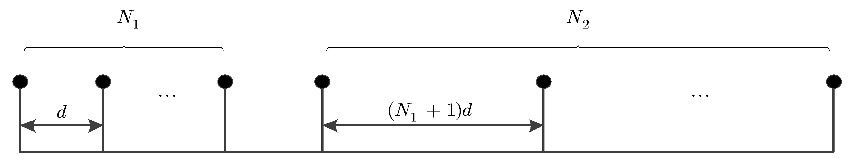
3. Tensor Model for a Nested Vector-Sensor Array
4. New Model for the Difference Co-Array
5. 2-D DOA and Polarization Parameter Estimation
5.1. Tensor-Based Spatial Smoothing
5.2. Uniqueness
5.3. Summary of the Proposed Method
6. Numerical Examples
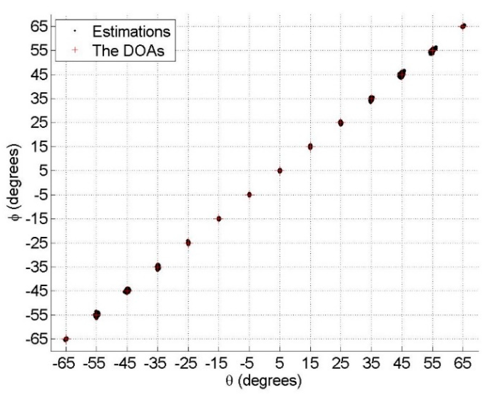
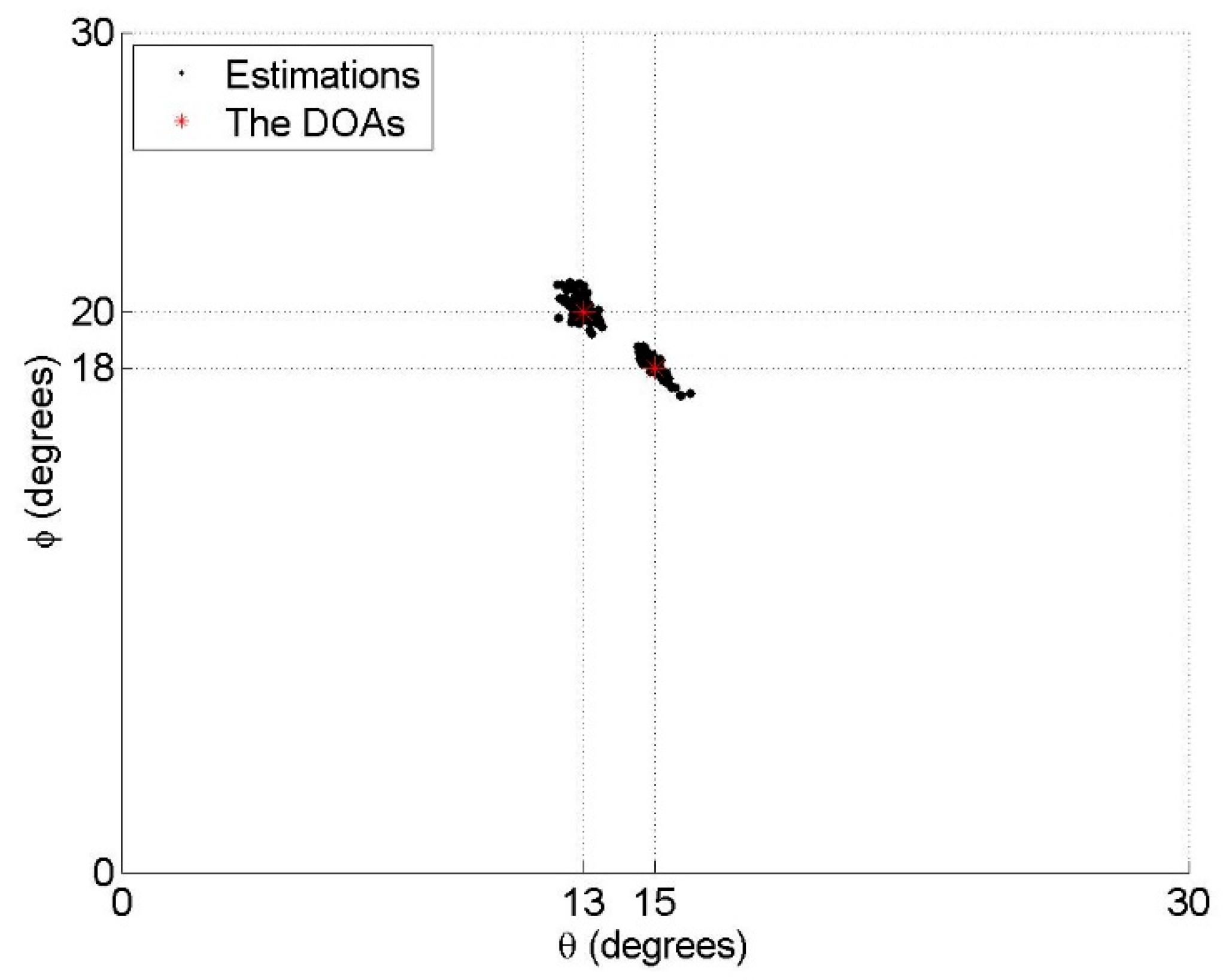
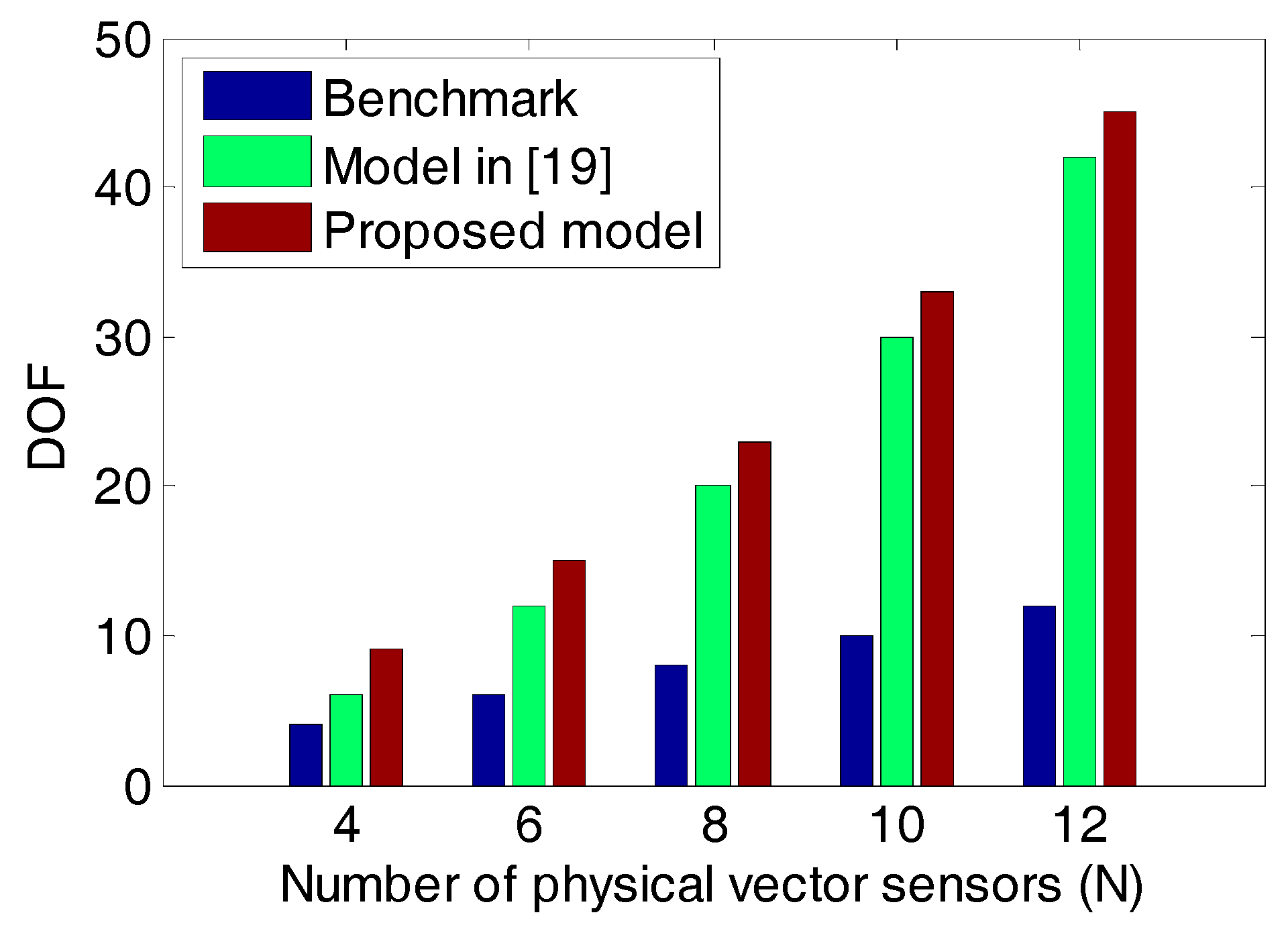
6.1. Identifiability of the Proposed Model
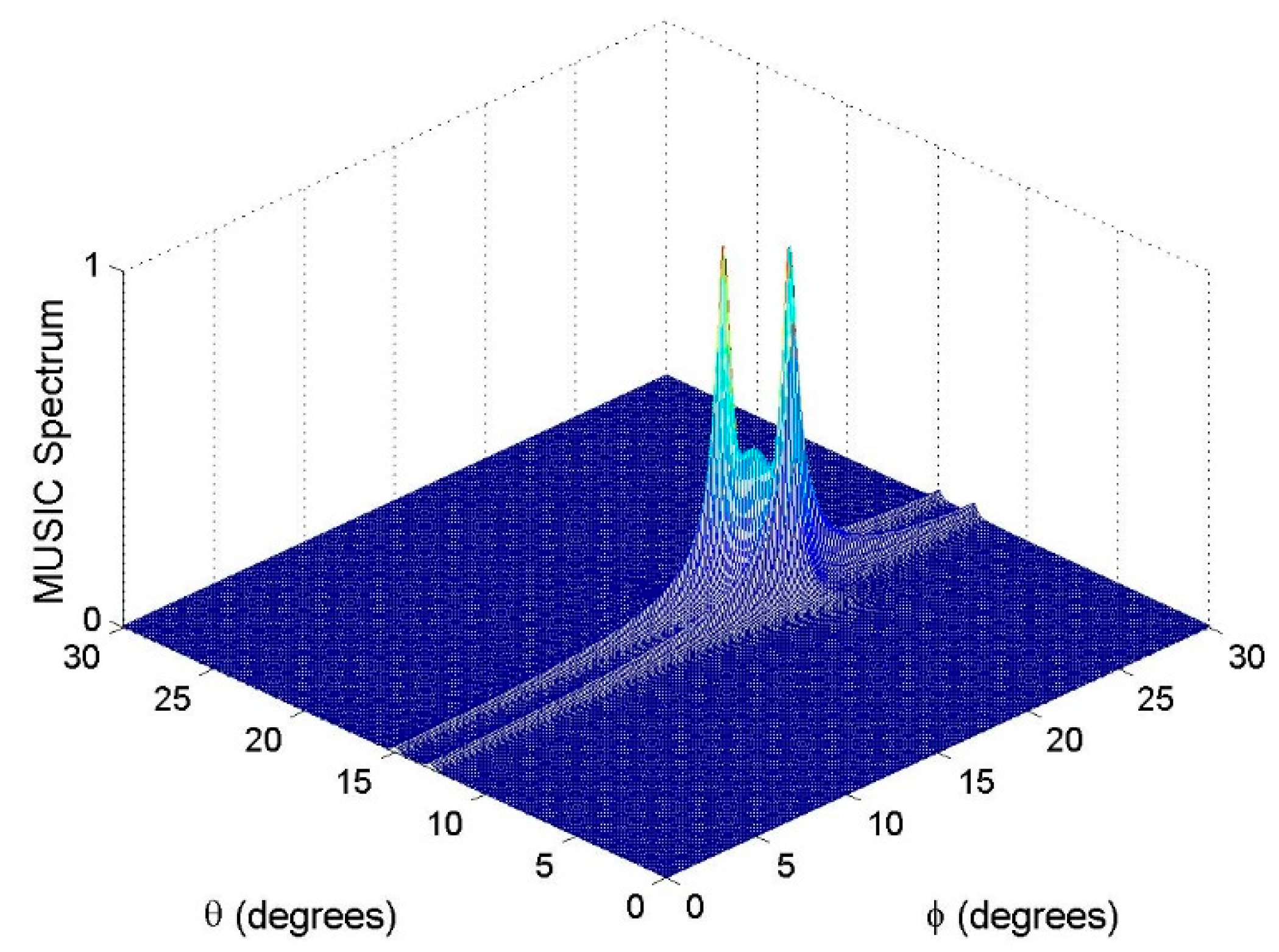
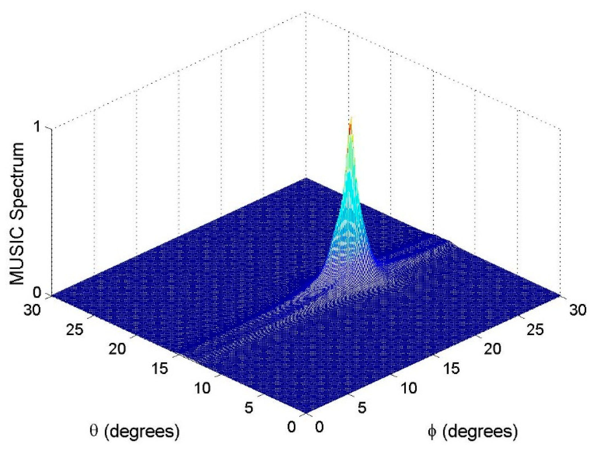
6.2. Resolution Performance
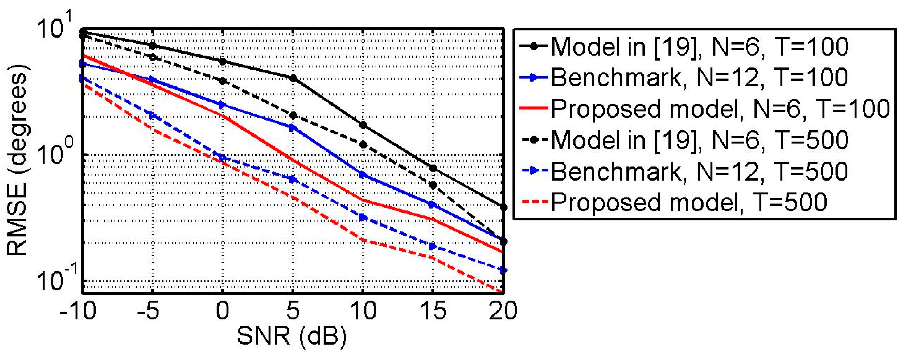
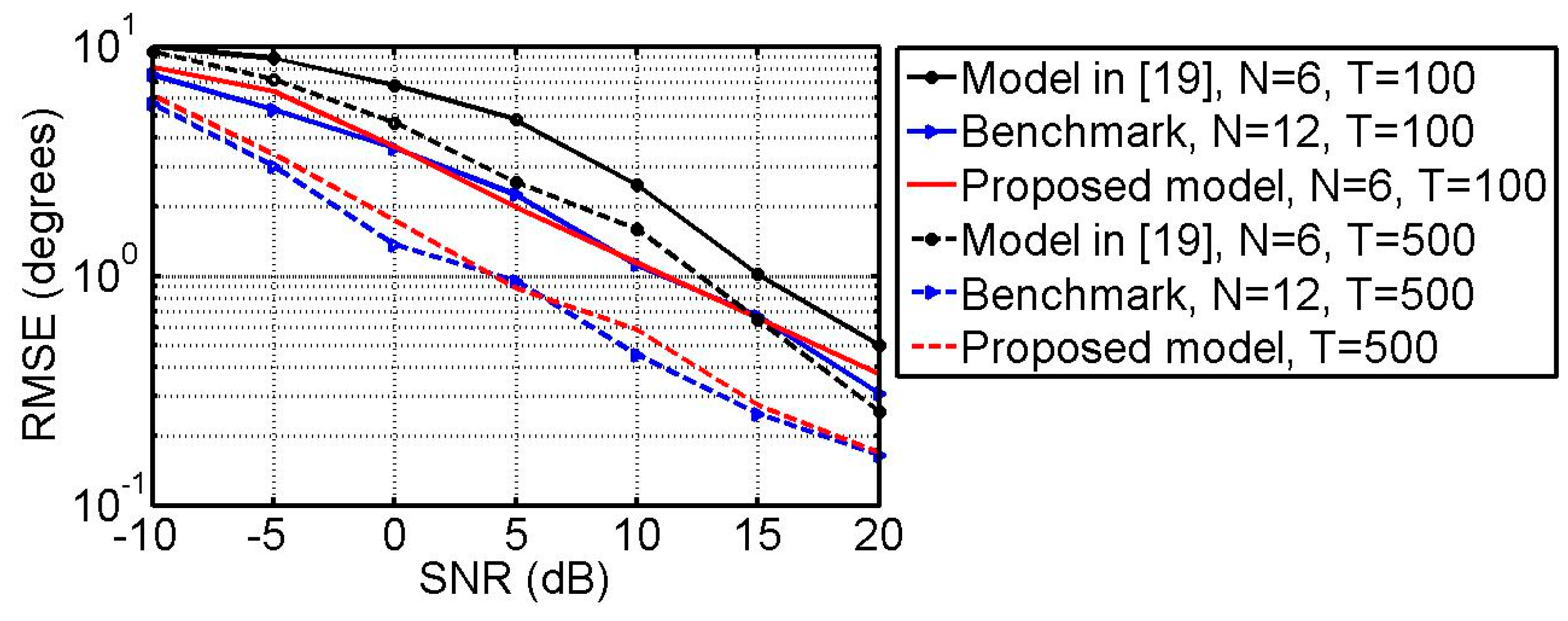
6.3. RMSE vs. SNR and Snapshots
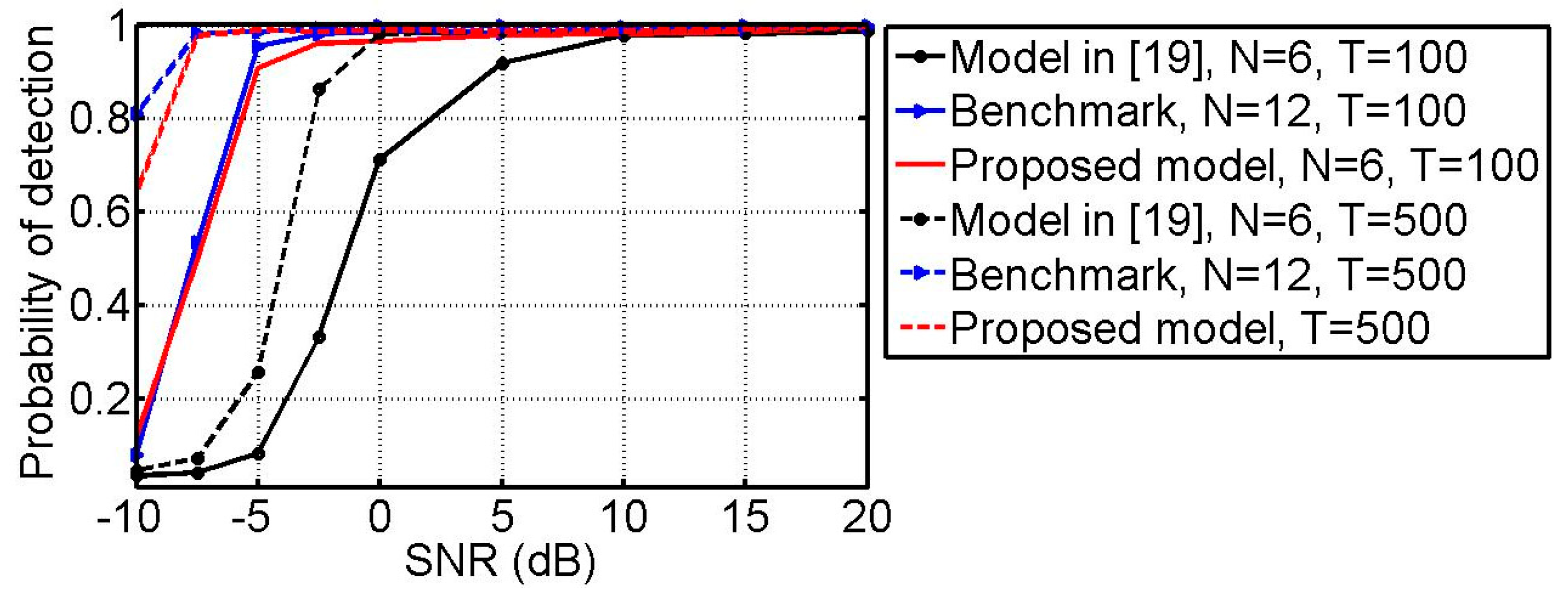
6.4. Detection Performance
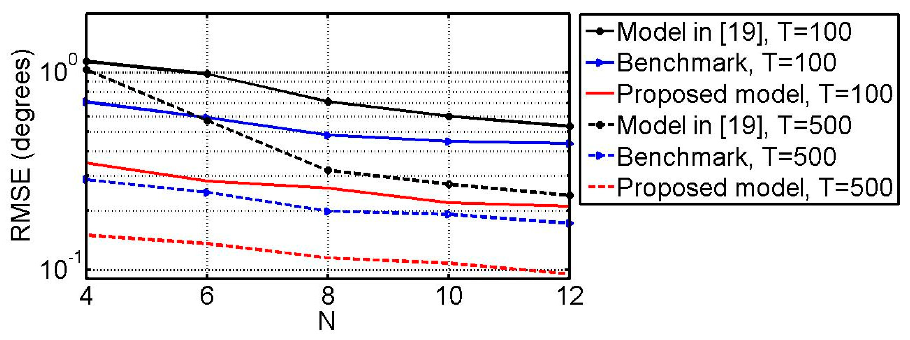
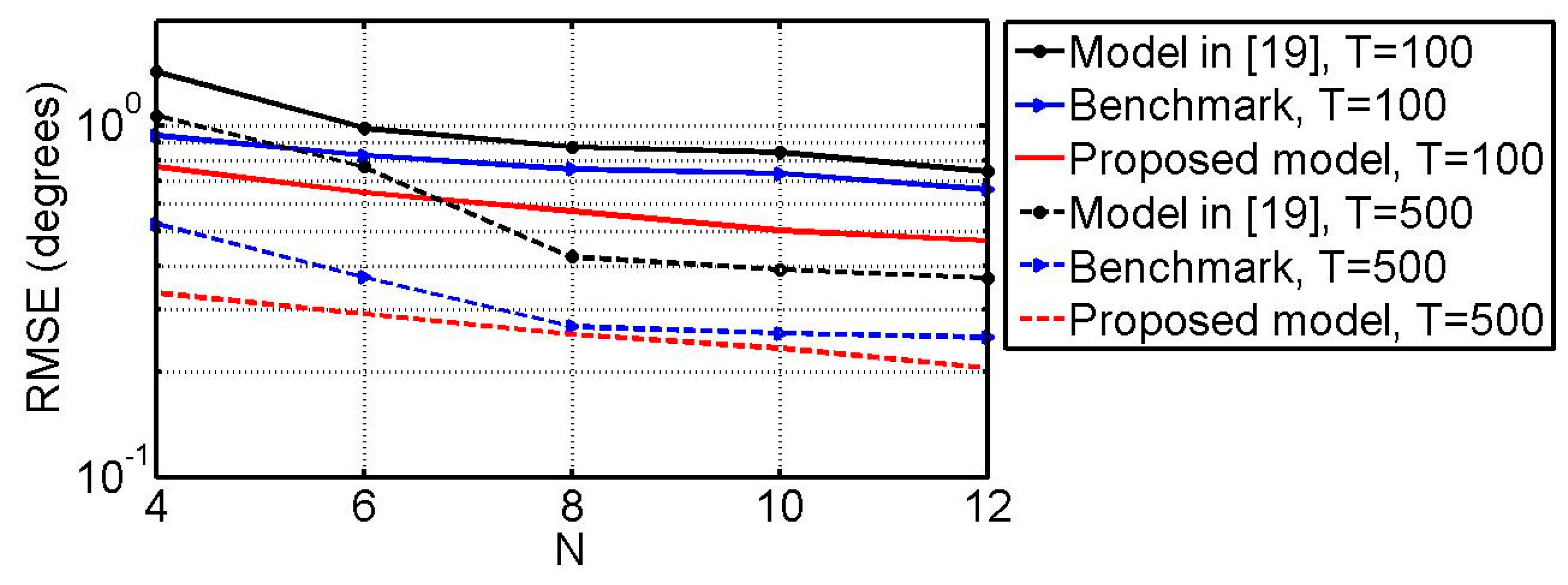
6.5 RMSE vs. N
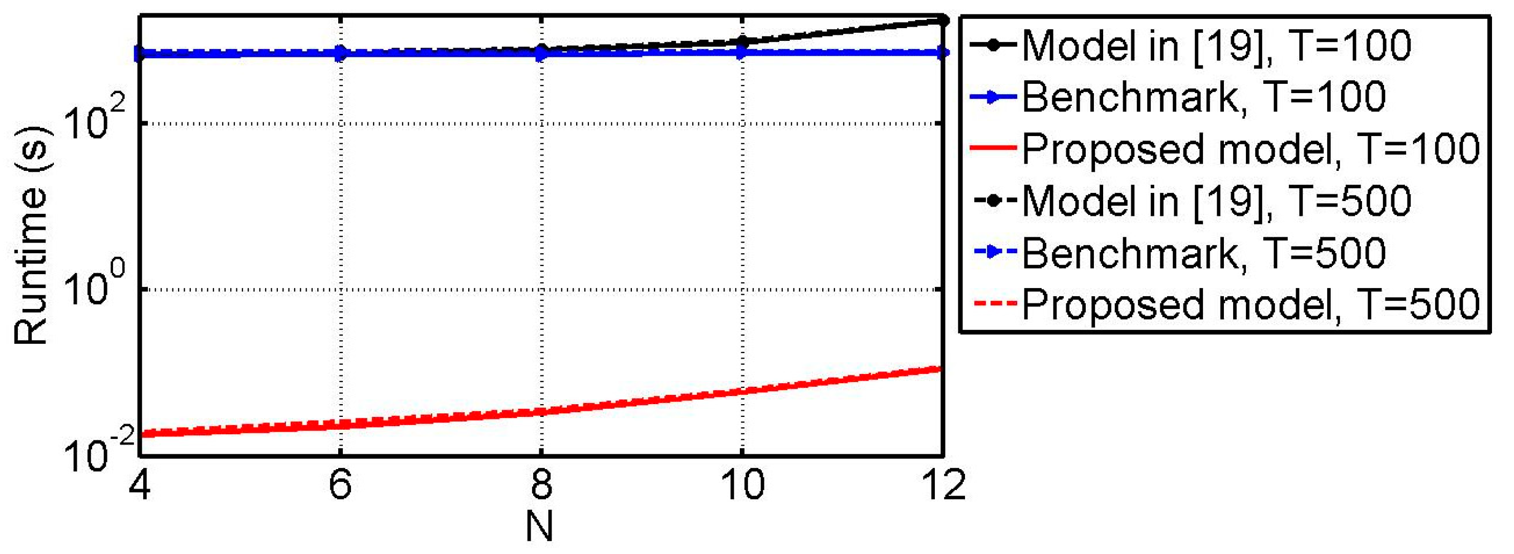
6.6. Runtime vs. N
7. Conclusions
Author Contributions
Funding
Conflicts of Interest
References
- Nehorai, A.; Paldi, E. Acoustic vector-sensor array-processing. IEEE Trans. Signal Process. 1994, 42, 2481–2491. [Google Scholar] [CrossRef]
- Nehorai, A.; Paldi, E. Vector-sensor array-processing for electromagnetic source localization. IEEE Trans. Signal Process. 1994, 42, 376–398. [Google Scholar] [CrossRef]
- Yuan, X. Estimating the doa and the polarization of a polynomial-phase signal using a single polarized vector-sensor. IEEE Trans. Signal Process. 2012, 60, 1270–1282. [Google Scholar] [CrossRef]
- Zhong, X.H.; Premkumar, A.B. Multiple wideband source detection and tracking using a distributed acoustic vector sensor array: A random finite set approach. Signal Process. 2014, 94, 583–594. [Google Scholar] [CrossRef]
- Zhao, A.; Bi, X.; Hui, J.; Zeng, C.; Ma, L. An improved aerial target localization method with a single vector sensor. Sensors 2017, 17, 2619. [Google Scholar] [CrossRef] [PubMed]
- Gu, C.; He, J.; Li, H.T.; Zhu, X.H. Target localization using mimo electromagnetic vector array systems. Signal Process. 2013, 93, 2103–2107. [Google Scholar] [CrossRef]
- Le Bihan, N.; Miron, S.; Mars, J.I. Music algorithm for vector-sensors array using biquaternions. IEEE Trans. Signal Process. 2007, 55, 4523–4533. [Google Scholar] [CrossRef]
- Liu, L.; Wang, L.; Zhang, Z. Vector-sensor-based signal parameter estimation by exploiting cpd of tensors. IEEE Sens. Lett. 2018, 2, 1–4. [Google Scholar] [CrossRef]
- Pal, P.; Vaidyanathan, P.P. Nested arrays: A novel approach to array processing with enhanced degrees of freedom. IEEE Trans. Signal Process. 2010, 58, 4167–4181. [Google Scholar] [CrossRef]
- Zhao, Y.H.; Zhang, L.R.; Gu, Y.B. Array covariance matrix-based sparse bayesian learning for off-grid direction-of-arrival estimation. Electron. Lett. 2016, 52, 401–402. [Google Scholar] [CrossRef]
- Pal, P.; Vaidyanathan, P.P. Nested arrays in two dimensions, part I: Geometrical considerations. IEEE Trans. Signal Process. 2012, 60, 4694–4705. [Google Scholar] [CrossRef]
- Alinezhad, P.; Seydnejad, S.R.; Abbasi-Moghadam, D. Doa estimation in conformal arrays based on the nested array principles. Digit. Signal Process. 2016, 50, 191–202. [Google Scholar] [CrossRef]
- Niu, C.; Zhang, Y.S.; Guo, J.R. Interlaced double-precision 2-d angle estimation algorithm using l-shaped nested arrays. IEEE Signal Process. Lett. 2016, 23, 522–526. [Google Scholar] [CrossRef]
- Zhang, L.; Ren, S.; Li, X.; Ren, G.; Wang, X. Generalized l-shaped nested array concept based on the fourth-order difference co-array. Sensors 2018, 18, 2482. [Google Scholar] [CrossRef] [PubMed]
- Yang, J.; Liao, G.S.; Li, J. Robust adaptive beamforming in nested array. Signal Process. 2015, 114, 143–149. [Google Scholar] [CrossRef]
- Han, K.Y.; Nehorai, A. Wideband gaussian source processing using a linear nested array. IEEE Signal Process. Lett. 2013, 20, 1110–1113. [Google Scholar]
- Han, K.Y.; Nehorai, A. Nested array processing for distributed sources. IEEE Signal Process. Lett. 2014, 21, 1111–1114. [Google Scholar]
- Han, X.; Shu, T.; He, J.; Yu, W. Polarization-angle-frequency estimation with linear nested vector sensors. IEEE Access 2018, 6, 36916–36926. [Google Scholar] [CrossRef]
- Han, K.; Nehorai, A. Nested vector-sensor array processing via tensor modeling. IEEE Trans. Signal Process. 2014, 62, 2542–2553. [Google Scholar] [CrossRef]
- Kolda, T.G.; Bader, B.W. Tensor decompositions and applications. SIAM Rev. 2009, 51, 455–500. [Google Scholar] [CrossRef]
- Boizard, M.; Ginolhac, G.; Pascal, F.; Forster, P. Low-rank filter and detector for multidimensional data based on an alternative unfolding hosvd: Application to polarimetric stap. EURASIP J. Adv. Signal Process. 2014, 2014, 119. [Google Scholar] [CrossRef]
- Li, Y.; Zhang, J.Q. Mode-r subspace projection of a tensor for multidimensional harmonic parameter estimations. IEEE Trans. Signal Process. 2013, 61, 3002–3014. [Google Scholar] [CrossRef]
- Sorensen, M.; De Lathauwer, L. Blind signal separation via tensor decomposition with vandermonde factor: Canonical polyadic decomposition. IEEE Trans. Signal Process. 2013, 61, 5507–5519. [Google Scholar] [CrossRef]
- Dong, Y.Y.; Dong, C.x.; Liu, W.; Chen, H.; Zhao, G.q. 2-d doa estimation for l-shaped array with array aperture and snapshots extension techniques. IEEE Signal Process. Lett. 2017, 24, 495–599. [Google Scholar] [CrossRef]
- Pal, P.; Vaidyanathan, P.P. Nested arrays in two dimensions, part II: Application in two dimensional array processing. IEEE Trans. Signal Process. 2012, 60, 4706–4718. [Google Scholar] [CrossRef]
- Rao, W.; Li, D.; Zhang, J.Q. A tensor-based approach to l-shaped arrays processing with enhanced degrees of freedom. IEEE Signal Process. Lett. 2018, 25, 1–5. [Google Scholar] [CrossRef]
- Kah-Chye, T.; Kwok-Chiang, H.; Nehorai, A. Linear independence of steering vectors of an electromagnetic vector sensor. IEEE Trans. Signal Process. 1996, 44, 3099–3107. [Google Scholar] [CrossRef]
- Hochwald, B.; Nehorai, A. Identifiability in array processing models with vector-sensor applications. IEEE Trans. Signal Process. 1996, 44, 83–95. [Google Scholar] [CrossRef]
- Lathauwer, L.D. Decompositions of a higher-order tensor in block terms—Part I: Lemmas for partitioned matrices. SIAM J. Matrix Anal. Appl. 2008, 30, 1022–1032. [Google Scholar] [CrossRef]
- Nion, D.; Sidiropoulos, N.D. Tensor algebra and multidimensional harmonic retrieval in signal processing for mimo radar. IEEE Trans. Signal Process. 2010, 58, 5693–5705. [Google Scholar] [CrossRef]
- He, Z.; Cichocki, A.; Xie, S.; Choi, K. Detecting the number of clusters in n-way probabilistic clustering. IEEE Trans. Pattern Anal. Mach. Intell. 2010, 32, 2006–2021. [Google Scholar] [PubMed]
- Cichocki, A.; Mandic, D.P.; Phan, A.H.; Caiafa, C.F.; Zhou, G.X.; Zhao, Q.B.; De Lathauwer, L. Tensor decompositions for signal processing applications. IEEE Signal Process. Mag. 2015, 32, 145–163. [Google Scholar] [CrossRef]


| The Proposed Method |
|---|
| Input: of the form (5). 1. Extract from . 2. Compute and , and built . 3. Compute and built . 4. Extract from according to (29), and built . 5. Compute and built . 6. Obtain , and from . 7. Obtain from . 8. Obtain , and from . Output: , , and . |
© 2018 by the authors. Licensee MDPI, Basel, Switzerland. This article is an open access article distributed under the terms and conditions of the Creative Commons Attribution (CC BY) license (http://creativecommons.org/licenses/by/4.0/).
Share and Cite
Rao, W.; Li, D.; Zhang, J.Q. A Novel PARAFAC Model for Processing the Nested Vector-Sensor Array. Sensors 2018, 18, 3708. https://doi.org/10.3390/s18113708
Rao W, Li D, Zhang JQ. A Novel PARAFAC Model for Processing the Nested Vector-Sensor Array. Sensors. 2018; 18(11):3708. https://doi.org/10.3390/s18113708
Chicago/Turabian StyleRao, Wei, Dan Li, and Jian Qiu Zhang. 2018. "A Novel PARAFAC Model for Processing the Nested Vector-Sensor Array" Sensors 18, no. 11: 3708. https://doi.org/10.3390/s18113708
APA StyleRao, W., Li, D., & Zhang, J. Q. (2018). A Novel PARAFAC Model for Processing the Nested Vector-Sensor Array. Sensors, 18(11), 3708. https://doi.org/10.3390/s18113708