1. Introduction
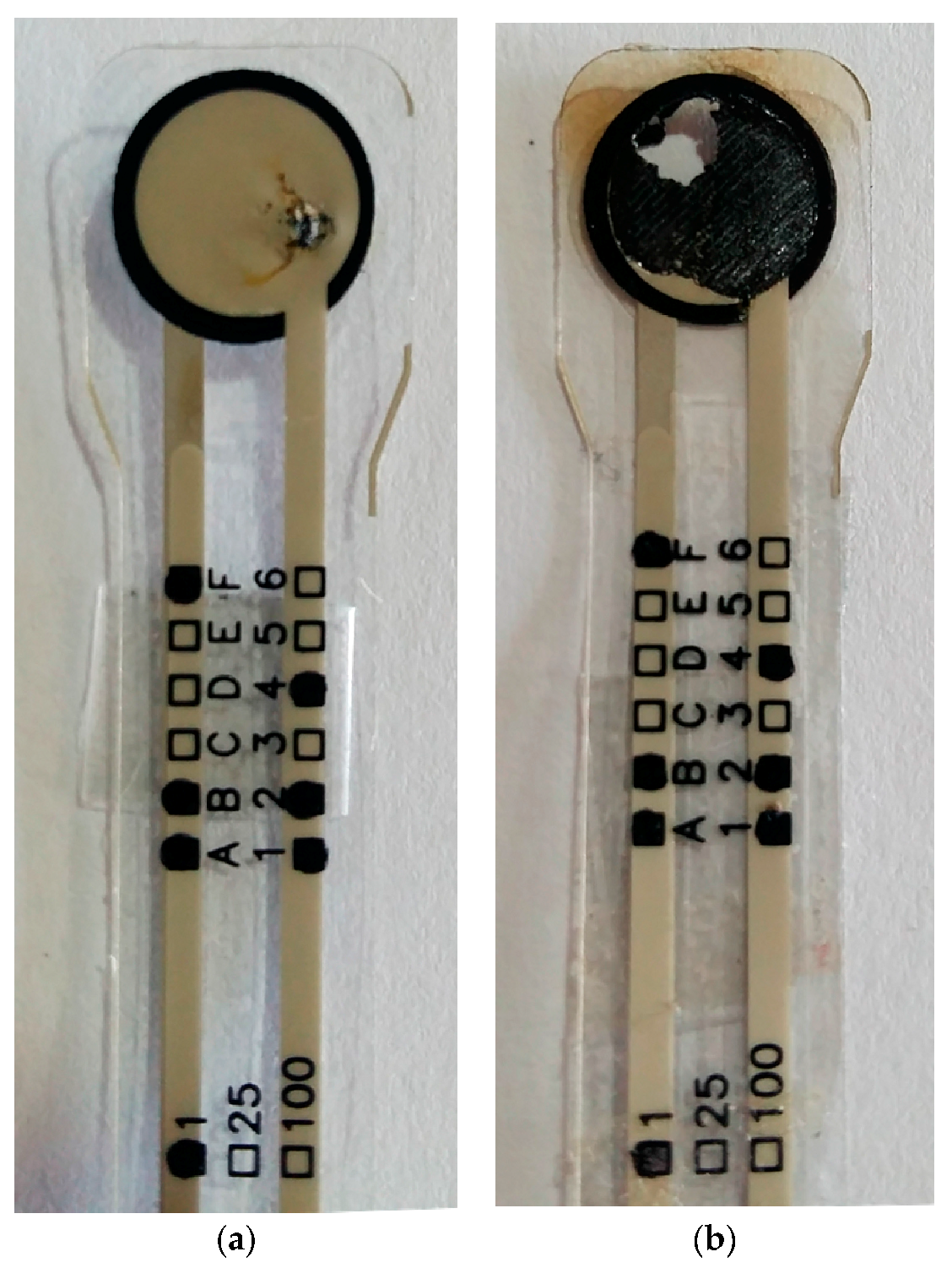
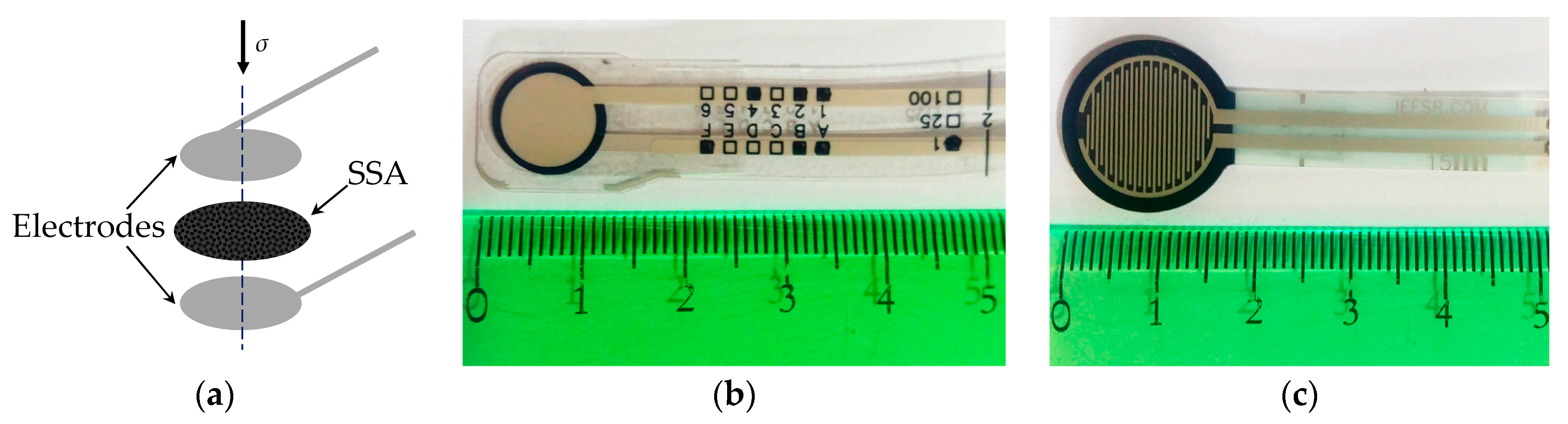
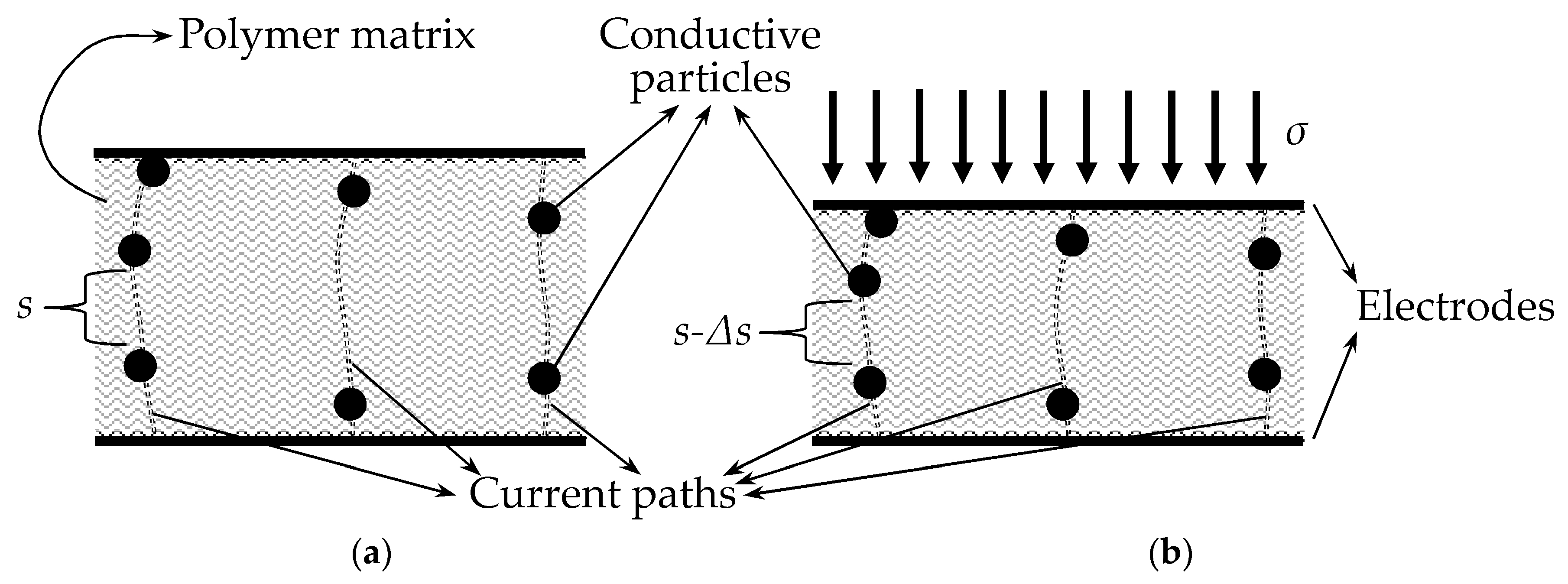
A Force Sensing Resistor (FSR) is a two-terminal passive device which exhibits a dramatic decrease in its electrical resistance when stress is exerted over the Sensor Sensitive Area (SSA). The SSA is usually made from conductive particles which are randomly dispersed in a non-conductive polymer resulting in a polymer composite; the SSA is later sandwiched between two metal electrodes to allow electrical measurements; the resulting device is an FSR as shown on the sketch of
Figure 1a and on the picture of
Figure 1b. This manufacturing process holds the designation of Traditional Sandwich Element (TSE). It is also possible to assemble an FSR using non-aligned electrodes (NAEE) or transverse electrodes (TEP) as the sensor on
Figure 1c. Wang et al. [
1,
2] have demonstrated that the location of the electrodes notably influences the creep behavior of FSRs.
The characterization of materials that can be used in the SSA manufacturing is currently an active research area. A broad range of materials have been evaluated as the non-conductive element in the fabrication of SSA, but elastomers, rubbers and polydimethylsilicone (PDMS) are the preferably chosen polymers as reported by Stassi et al. [
3]. Likewise, conductive particles can be obtained from different metals, such as Nickel or Cooper, with particles sizes within the range of tens of nanometers up to a few micrometers [
4,
5]. Carbon black and carbon nanotubes have also been implemented as conductive phases in the insulating matrix [
6,
7].
As can be noticed from the previously cited studies, the research possibilities are vast within the manufacturing of SSA since they comprise multiple design parameters, such as: electrode configuration (TSE, NAEE, TEP and hybrid topologies), type of insulating material (elastomer, rubber, resins, metal-oxides and thermostable polymers), and properties of the conductive particles (material and size of particles, mass ratio of the conductive particles to the insulating material). Therefore, multiple designations have been given in literature to these kinds of smart materials, but the key aspect to categorize them has been placed on the type of insulating element. Hence, the most common designations that can be found in regard to the SSA are: conductive polymer [
8], semiconductive polymer [
9], and rubber/elastomer/PDMS composite with conductive nanoparticles [
10]. Likewise, the phenomenological designation of piezoresistive sensor is also common in literature [
11]. Henceforth in this article, the designation of polymer composite is used when discussing about the material employed in the manufacturing of the SSA.
On the other hand, the designation of FSR has been preferably used to refer to off-the-shelf sensors which can be readily integrated into a given application. Several models of FSRs are currently commercially available [
12], but the most-widely used brands of FSRs are the family of FlexiForce A201/A401 sensors, manufactured by Tekscan, Inc. (Boston, MA, USA) [
13,
14,
15] and the family of FSR 40X sensors manufactured by Interlink Electronics, Inc. (Westlake Village, CA, USA) [
16,
17,
18]. Pictures of both sensors are shown in
Figure 1b,c, respectively. Both manufacturers offer a broad range of force-sensing solutions in terms of nominal force ranges, sensor dimensions, interface circuits and end-user software, such as the popular F-scan in-shoe analysis system which is intended for gait analysis [
19].
It must be recalled that the designation of thin insulating film/layer has been used in literature to describe and model the conduction mechanisms of polymer composites [
20,
21]. A polymer composite operates on the basis of either quantum tunneling or percolation; although both phenomena can actually occur simultaneously [
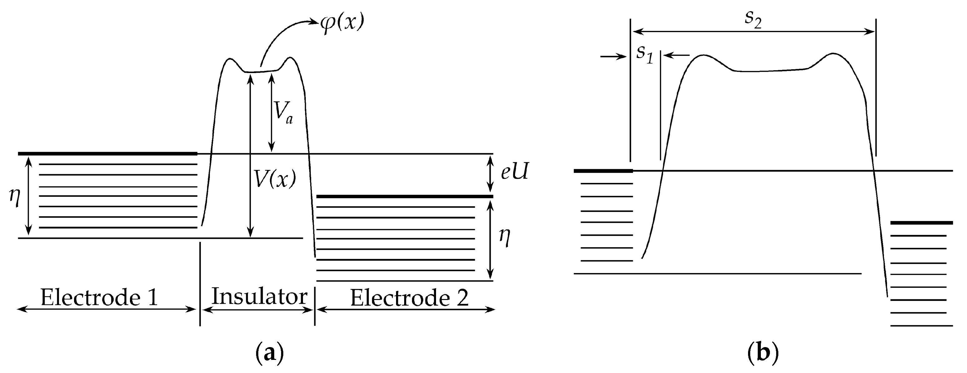
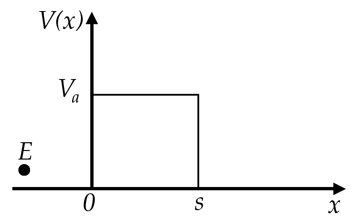
3]. When subjected to stress, the average inter-particle separation of the polymer composite changes, and consequently, the electrical resistance of the SSA varies. In the 1960s, Simmons [
21] provided the foundation physics for the quantum tunneling conduction of thin insulating layers. His model accurately predicted the current-voltage (
I-U) relationship that Fisher and Giaever [
20] have previously reported when characterizing thin insulating film layers fabricated from aluminum oxide. Later models have been developed based upon the original formulation from Simmons [
21]; such models are more complex as they embrace additional parameters such as: particle size on the conductive filler [
9], creep response of the polymer composite [
22] and mass ratio of the conductive phase to the insulating matrix [
23].
The afore-cited models of Kalantari et al. [
9], Zhang et al. [
22] and Wang et al. [
23] share one thing in common; they describe the relative variation of the electrical resistance when the polymer composite is subjected to stress. The relative variation of resistance is represented in regard to one of the following magnitudes: the original resistance immediately upon the application of stress [
9,
22], or the original resistance when the polymer composite is unloaded [
23]. In practice, this implies that the aforementioned models rely upon experimental readings to describe the
I-U, stress-resistance (
σ-R), and the time-resistance (
t-R) relationships. Nonetheless, the original formulation from Simmons [
21] does not comprise any type of experimental readings. Instead, the model from Simmons [
21] is based upon physical constants, e.g., electron mass and charge, Planck constant, and upon different properties from the conductive and the non-conductive elements, e.g., average inter-particle separation and work function of each element.
The main contribution of this article is to derive a theoretical model capable of predicting the absolute
I-U and
σ-R relationships of polymer composites and FSRs when subjected to stress. The proposed model has mainly two differences with the aforesaid studies from Kalantari et al. [
9], Zhang et al. [
22] and Wang et al. [
23] as next mentioned: first, as the proposed model describes the absolute
I-U and
σ-R relationships, it does not require experimental measurements of the electrical resistance; this is important because the proposed model is capable of making predictions relying solely on simulation, and second, the proposed model embraces two additional parameters that the above mentioned studies have ignored or have assumed as constant; these are: the stress-dependent behavior of the area (
A) for quantum tunneling conduction, and the influence of the input voltage (
U) over the electrical resistance.
Finally, it must be recalled that FSRs are made from a polymeric binder, and thus, a rheological behavior is observed in the electrical resistance of the device [
24]. The rheological response of polymers yields inaccuracies that fall within the following types of errors: hysteresis [
25], creep [
26], and loss of sensitivity under continuous operation [
27,
28]. In this article, and for the sake of paper length, the rheological behavior of polymer composites is not taken into account which is a limitation of the proposed model. Similarly, this work is based upon the Simmons model [
21] for the current conduction through thin insulating layers which was derived on the basis of two approximations: the WKB and approximated evaluation of integrals, and thereby, the experimental data do not perfectly fit the proposed model.
The rest of this paper is organized as follows: the conduction mechanisms of polymer composites and FSRs are described in
Section 2 with special emphasis on the quantum tunneling effect and the contact resistance. In
Section 3, a review is presented for the models that predict the relative variation of the
I-U and
σ-R relationships of polymer composites. In
Section 4, the derivation of the proposed model is addressed, followed in
Section 5 by a presentation of the experimental results, and conclusions on
Section 6. Two appendixes have been included in this article:
Appendix A presents a review on the concepts of current density (
J) electrical current (
I), and electrical resistance per unit area (
RA). A full understanding of such concepts is required to comprehend Simmons’ model [
21].
Appendix B describes the steps followed by Simmons to derive his model.
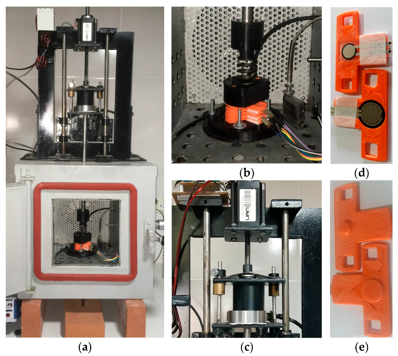
The tests conducted in this study were performed over A201-1 and FSR 402 sensors, manufactured by Tekscan, Inc. (South Boston, MA, USA) and Interlink Electronics, Inc. (Camarillo, CA, USA), respectively. The nominal range of both sensors is 4.5 N and 20 N, respectively.
3. A Review on the Models that Predict the I-U and σ-R Relationships of Polymer Composites
In this section, it is presented a brief description of the models that predict the relative variation of resistance in polymer composites. The models of Zhang et al. [
22], Wang et al. [
23] and Kalantari et al. [
9] are individually addressed. The original notation from the authors has been kept for all symbols except for the parameters describing the sensor area. This was necessary for two reasons: the aforesaid authors do not employ a unique nomenclature, and second, a distinction was introduced in this article for the sensor physical area,
AFSR, and the effective area for tunneling conduction,
A. The start point for all the models is the following equation:
where
R(
σ) is the composite resistance as a function of the applied stress,
L is the number of particles forming one conductive path (series-connected),
S is the total number of conductive paths,
RPol is given by Equation (9), and
Rpar is the resistance of a single conductive particle. Zhang et al., Wang et al. and Kalantari et al. stated that
Rpar is negligible when compared to the resistance of the polymer composite—the tunneling resistance
RPol—and thus, Equation (12) can be simplified to:
Let
R0 be the resistance of the polymer composite at rest state, i.e., when
σ = 0. In practice,
R0 is experimentally measured with a multimeter before sensor testing [
9,
22,
23]. By replacing Equation (9) at the Equation (13), and dividing by
R0, the following expression can be obtained:
where
s0 is the inter-particle separation in the polymer composite at sensor rest and
s is the inter-particle separation when subjected to stress. The quotient
L/
S has been removed from the Equation (14), because Zhang et al. and Kalantari et al. considered that such a quotient is force independent. Conversely, Wang et al. stated in their model that the number of conductive paths actually grows as the applied stress increases. The authors’ proposal on this topic is addressed on
Section 4. Variations of Equation (14) have been developed by Zhang et al., Wang et al. and Kalantari et al. as next described:
3.1. The Model of Zhang et al. [22]
Zhang et al. were the first to propose a model for the relative variation of resistance in polymer composites. Later models from Kalantari et al. and Wang et al. are based on the original formulation of Zhang et al., and hence, special emphasis is placed on describing the original formulation from Zhang et al., whereas the other two models are briefly described.
Previous attempts on modeling the piezoresistance of polymer composites have been carried out by Carmona et al. [
37] and Ruschau et al. [
35]. However, it must be remarked that the Carmona’s derivation was obtained on the basis of assuming classical percolation conduction through the polymer composite, whereas Ruschau et al. put more emphasis on the tunneling resistance at the contacts but a theoretical model for such phenomenon was not provided. Conversely, the model from Zhang et al. and their successors were obtained on the basis of quantum tunneling. Zhang et al. developed two models for the relative variation of resistance. The first model is focused on static forces whereas the second predicts the creep response of polymer composites.
Given the compressive modulus (M) of the insulating polymer matrix subjected to stress, σ. The strain (ε) can be found from the quotient ε = σ/M.
Given the inter-particle separation in the polymer composite at rest state,
s0. An expression for
s0 can be found from the particle diameter (
D) and filler volume fraction (
θ) as follows:
The filler volume fraction can be understood as the density ratio of the conductive nanoparticles to the insulating polymer matrix, readers may refer to Equation (19) at [
23] for further details on this topic. The relationship between the inter-particle separation,
s, and strain,
ε, can be expressed as:
A combination of Equations (9), (15) and (16) yields the first model of Zhang et al. in regard to the electrical resistance at sensor rest,
R0. The designation “in regard to
R0” implies dividing the resulting equation by
R0 as in Equation (14).
Three important facts can be yielded from Equation (17); first note that it is only capable of modeling the relative variation of resistance in regard to R0, second, it is assumed that the effective area for tunneling conduction is held constant regardless of σ, hence, the quotient A(σ)/A0 is not included because Zhang et al. assumed that A(σ) = A0, and third, Equation (17) predicts a voltage-independent behavior for R(σ).
The second model was obtained on the basis of the Nutting equation that relates sensor strain with time:
where
ε0 is the original strain immediately upon the application of stress,
ψ and
n are constants estimated on an empirical basis from a known-input stress. The time dependence of
s under conditions of constant stress can be calculated from:
Finally, the second model can be obtained by combining Equations (9) and (19) in regard to
R0:
Explicit time dependence on Equation (20) is possible by substituting Equation (18) on the time-dependent strain,
ε(
t). Likewise, the expression for
s0 can be also included in the second model from Zhang et al. as next:
3.2. The model of Wang et al. [23]
Wang et al. have developed several models to describe the piezoresistance behavior of polymer composites [
1,
6,
7,
23,
38]. However, the contribution from [
23] is the most relevant because it comprises multiple parameters in regard to the spatial distribution of the conductive nanoparticles, for such reason, such contribution is here described.
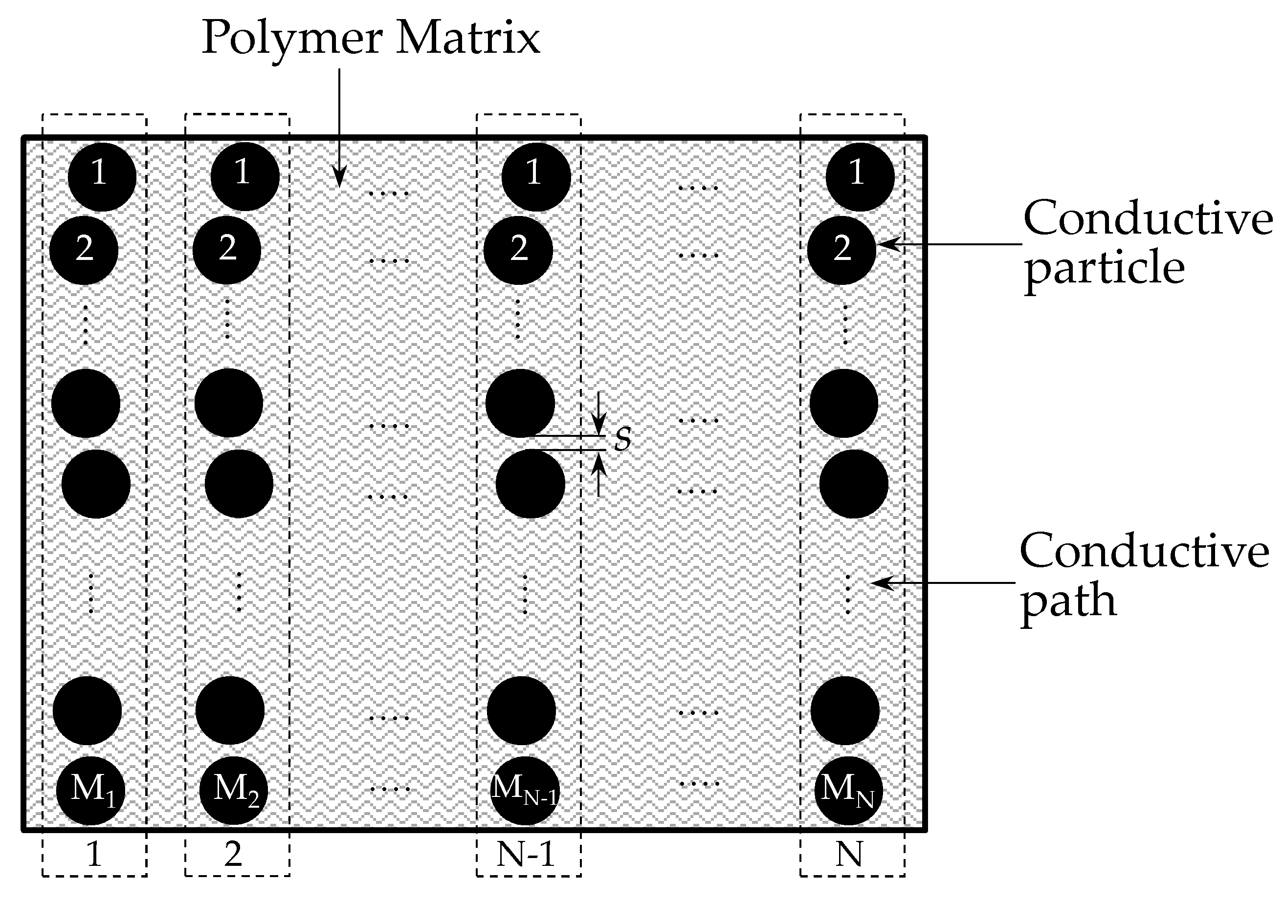
Given an insulating polymer matrix with
N paths for current conduction, the following equation can be stated for the electrical resistance of a polymer composite:
where
s stands for the inter-particle separation and
K represents the total number of particles along a conductive path as shown in
Figure 7. Equation (22) was obtained from (9) with the addition of the operands
K and
N to take into account the multiple conductive paths. Note that Equation (22) embraces dependence upon the area
A, and also, dependence upon the number of conductive paths,
N. However, the dependence upon
A is later discarded by Wang et al. as the final model assumes the relative variation of resistance (
Rr(
σ)) as:
where
Rs(
σ) is the electrical resistance of a single conductive path under stress. On the other hand, the following magnitudes, related to the rest state,
Rs(0),
R(0),
N(0) are the resistance of a single conductive path, the resistance of the whole polymer composite and the number of conductive paths, respectively. Note that the dependence on
A has been discarded on Equation (23), but the dependence on the quotient
N(
σ)/
N(0) remains. To authors’ criteria; this is the main contribution proposed by Wang et al. [
23] since the quotient
N(
σ)/
N(0) was useful to model the response of polymer composites working on the basis of percolation, readers may refer to Equation (21) at [
23]. It must be remarked that the percolation phenomenon is not addressed in this article, because quantum tunneling is the predominant conduction mechanism for the A201-1 and FSR 402 sensors.
Finally, note from Equation (23) that a voltage-independent behavior is assumed, and just as the previous formulation from Zhang et al. [
22], the model relies upon experimental measurements of the electrical resistance at sensor rest,
R(0).
3.3. The model of Kalantari et al. [9]
The theoretical formulation of Kalantari et al. is quite similar to the model of Zhang et al
. [
22], with the difference that the contact resistance,
RCon, was included in the model. By combining the expressions for the contact resistance, Equations (10) and (11), with the Zhang et al. formulation at Equation (17), the initial proposal from Kalantari et al. can be obtained as:
where all the symbols from Equation (24) have the same meaning as from the Zhang et al. formulation in
Section 3.1. A description for the symbols
ρ1, ρ2,
F and
H was already presented on
Section 2.3.
The main difference between the formulation of Zhang et al. and Kalantari et al. is that the latter employed the Zener rheological model [
24] to describe the time dependence of strain,
ε, whereas the former employed the nutting equation from Equation (18). The relationship between strain,
ε, and force,
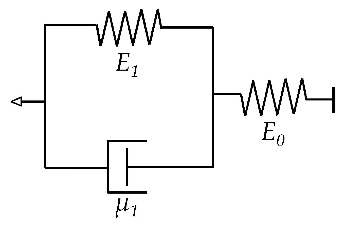
F, for a Zener element is given by:
where
E0,
E1 and
μ1 are the elasticity and viscosity constants from the Zener element shown in
Figure 8. The factor
AFSR is the corresponding area of the force sensor, which must not be confused with the effective area for tunneling conduction,
A. Readers may refer to
Appendix A for more details regarding this topic. Finally the model proposed by Kalantari et al. can be obtained by replacing
ε in Equation (24) for the time-dependent
ε(
t) as in Equation (25). The final expression is presented below:
Following with the trends of Zhang et al. [
22] and Wang et al. [
23], the model from Kalantari et al. also relies upon measurements of the electrical resistance at sensor rest, see the
R0 factor at Equations (24) and (26). Likewise, the input voltage,
U, and the area
A are not considered as parameters in either equation.
4. Proposal of a New Model for the Current-Voltage and the Stress-Resistance Relationships of FSRs
With the aim of avoiding any possible confusion, a different nomenclature is henceforth used in the derivation of the proposed model; this was mandatory because new mathematical expressions are introduced in this section for the resistance of the polymer composites,
RPol, and the contact resistance,
RCon. It must be remarked that multiple expression for
RPol were presented in
Section 3 as a part of the models from Zhang et al. [
22], Wang et al. [
23] and Kalantari et al. [
9]. Likewise, an expression for
RCon was already given in Equation (11).
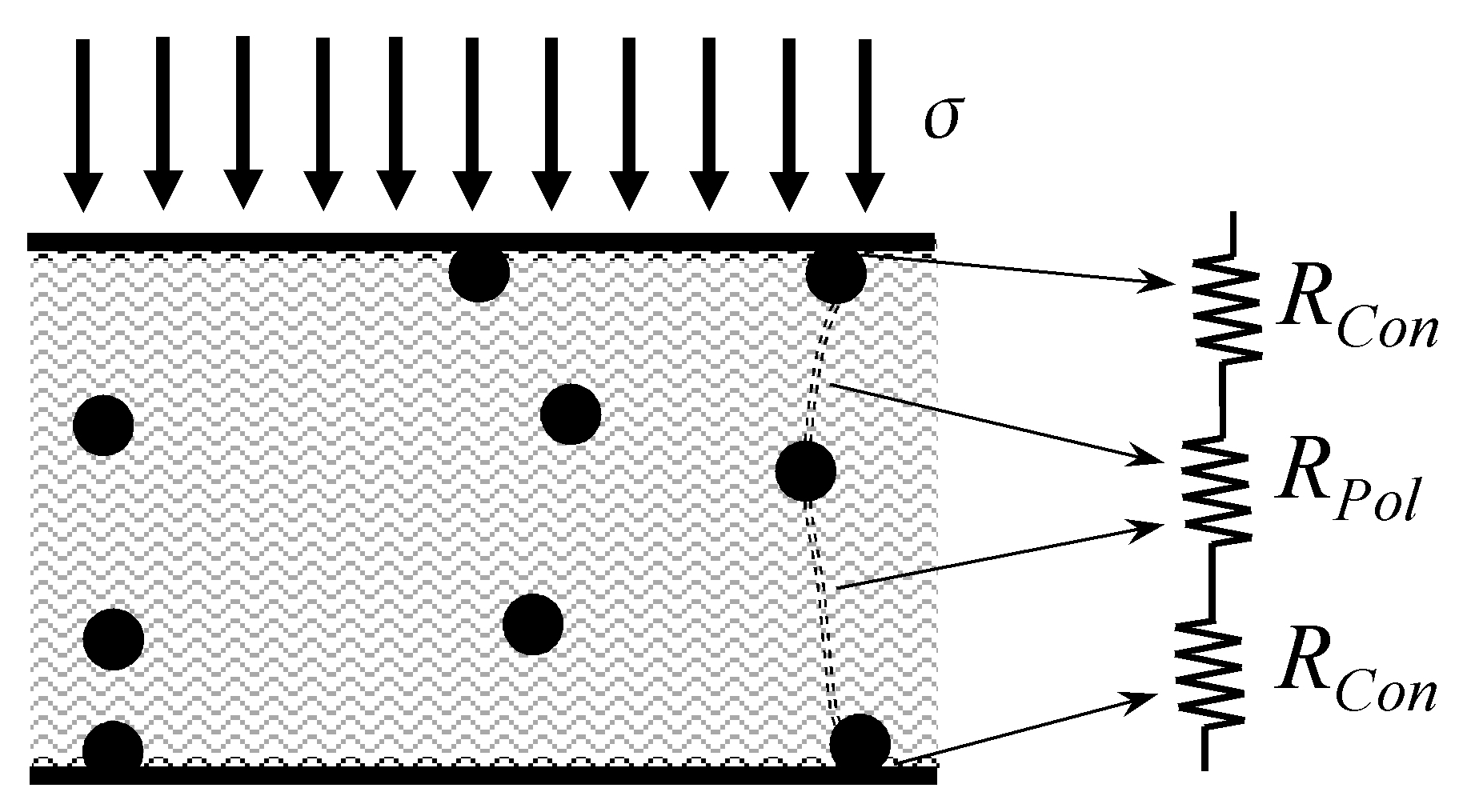
The formulation from Equation (10) is the start point for the proposal of the new model, but a different nomenclature is henceforth used below:
where
RFSR is the total resistance across the FSR comprising a series connection between the bulk resistance (
Rbulk) and the contact resistance (
Rc). The same sketch from
Figure 5 can be used to represent the series connection of
Rc and
Rbulk with the proviso that
RCon has been re-labeled as
Rc and
RPol has been re-labeled as
Rbulk. Note that the same current
I flows through both resistances. Hence, the following expression is yielded if Equation (27) is multiplied by
I:
In previous sections
U has been employed to refer to the input voltage;
U has been also used for the voltage across the thin insulating film, such a designation is enough for [
9,
21,
22,
23], but for the sake of this paper, it turns out to be insufficient because when operating on the basis of Equations (27) and (28), the input voltage—henceforth labeled as
VFSR—is split between the voltage across the polymer composite (
Vbulk), and the voltage across the contact resistance (
VRc). For such reason,
U is no longer used in this article, but
VFSR,
Vbulk and
VRc are used instead.
4.1. New Proposed Model for the Resistance of Polymer Composites, Rbulk, and the Effective Area, A
The proposed model embraces two additional parameters: the stress-dependent area,
A, and the voltage across the polymer composite,
Vbulk. It must be stated that the distinction presented in
Section 2.2 in regard of the difference between polymer composites and FSRs. In this Section, the contact resistance existing between the electrodes and the conductive particles is deliberately omitted, but in
Section 4.3, a combined model for
Rc and
Rbulk is presented.
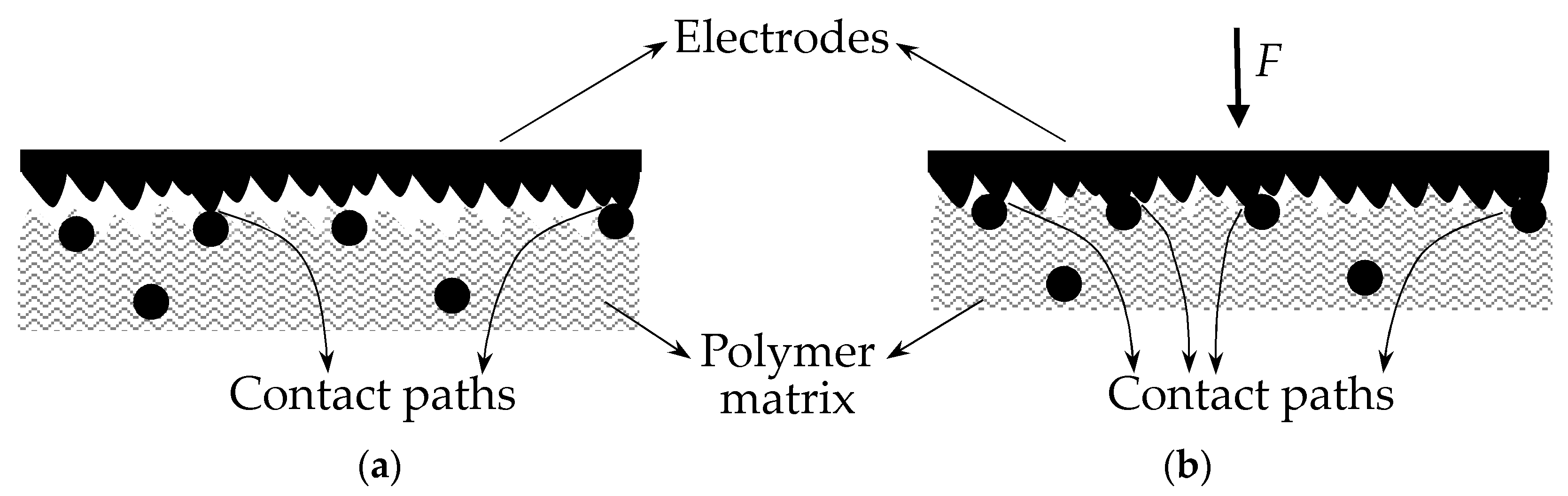
Let
A(
σ) be the effective area for the electrons to cross the potential barrier as a function of the applied stress with the following general form:
where
A0 is the effective area for tunneling conduction at rest state, and
f(
σ) is a stress dependent function that describes the increase in the number of conduction paths—and hence of the effective area—as the applied stress increases; such a phenomenon was previously depicted in
Figure 6. for the case of FlexiForce and Interlink sensors. The best suited form for
f(
σ) was found to be a power function:
It must be pointed out that Equation (30) has been proposed after testing several models on the experimental data from the A201-1 and FSR 402 sensors. Thus, Equation (30) cannot be assumed as a general model for the effective area of any piezoresistive sensor. Different forms of
f(
σ) could be proposed for custom-made sensors and for other sensor brands. However, the power-law from Equation (30) is quite similar to the behavior of the contact resistance; this similarity is later discussed in
Section 4.2.
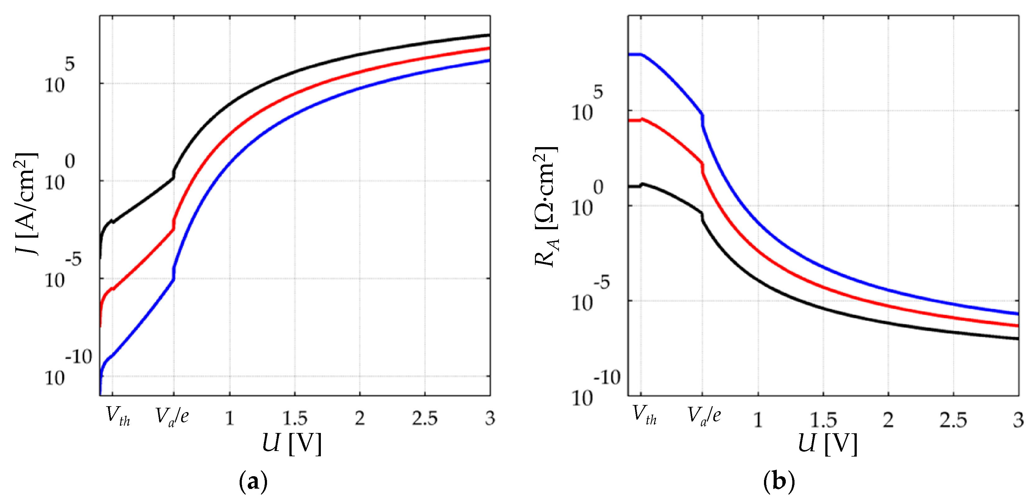
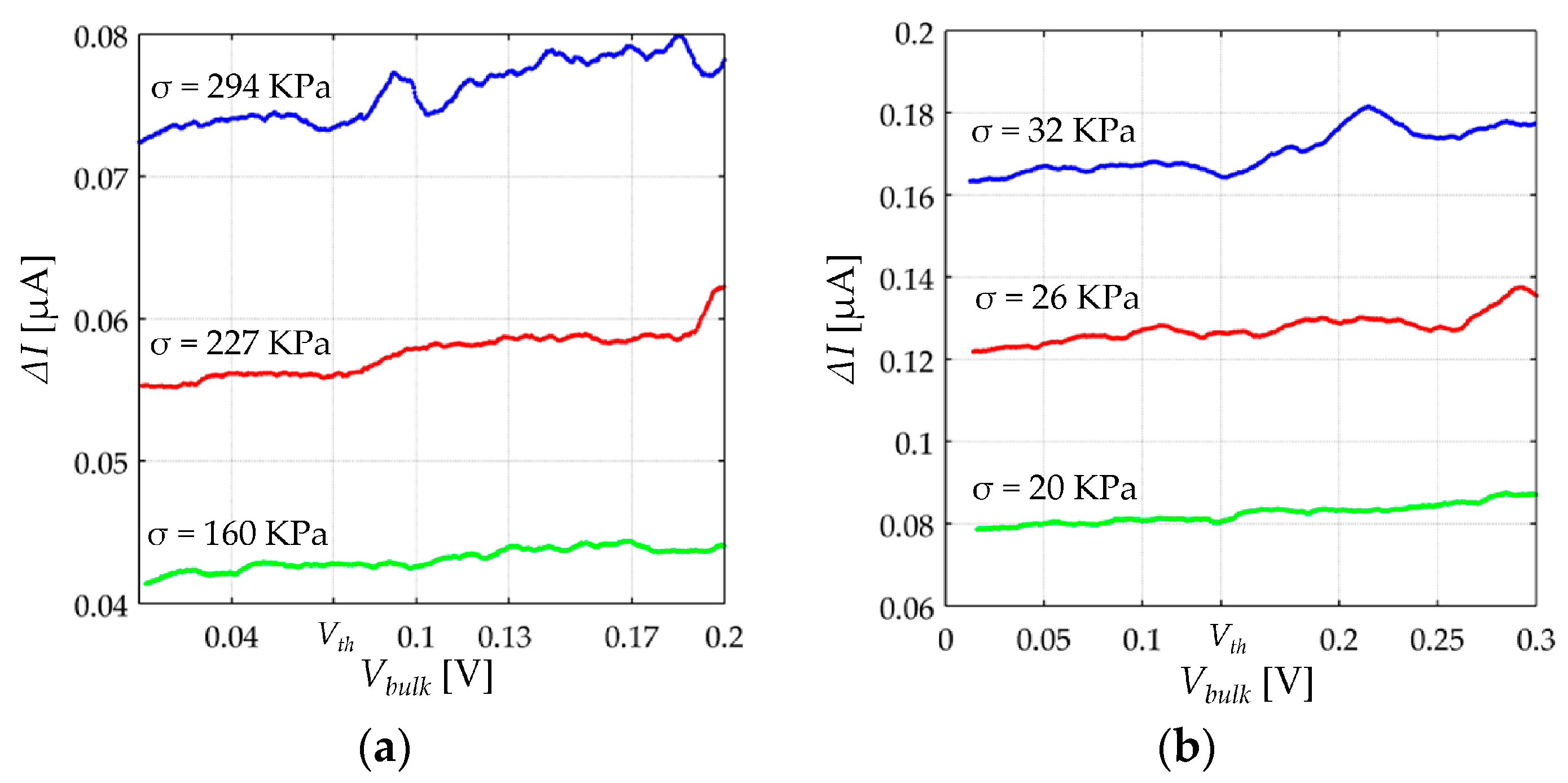
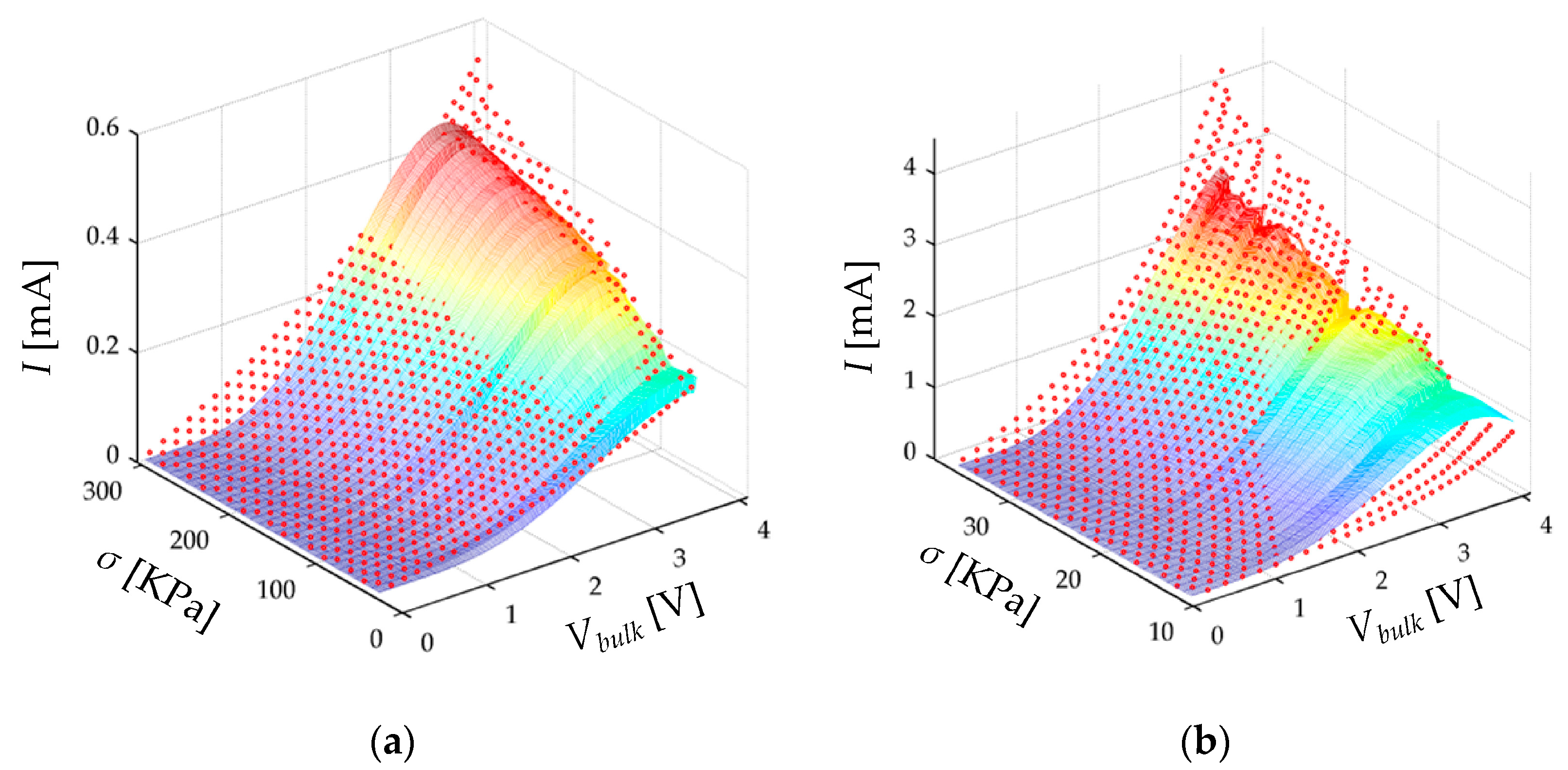
Variations in
Vbulk modify
Rbulk in a highly non-linear fashion as previously shown in the simulation plot of
Figure 4b. When
Vbulk is in the millivolt range,
Rbulk exhibits an ohmic behavior. When
Vbulk is increased beyond the millivolt threshold,
Vth, a decrease in
Rbulk is expected for incremental values of
Vbulk. Finally, when
Vbulk is greater than the height of the potential barrier,
Va/e, a small increment in
Vbulk yields a dramatic increase in sensor current. These statements have been experimentally demonstrated by Fisher and Giaever [
20].
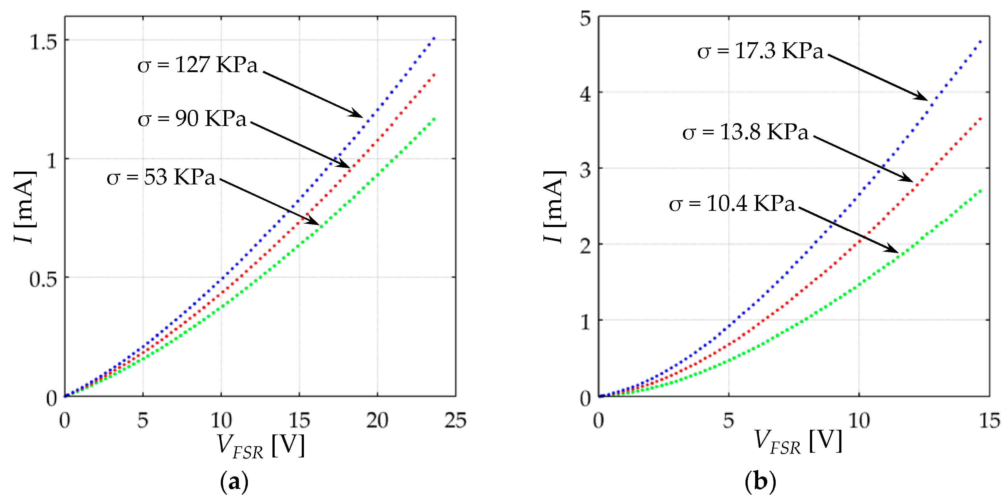
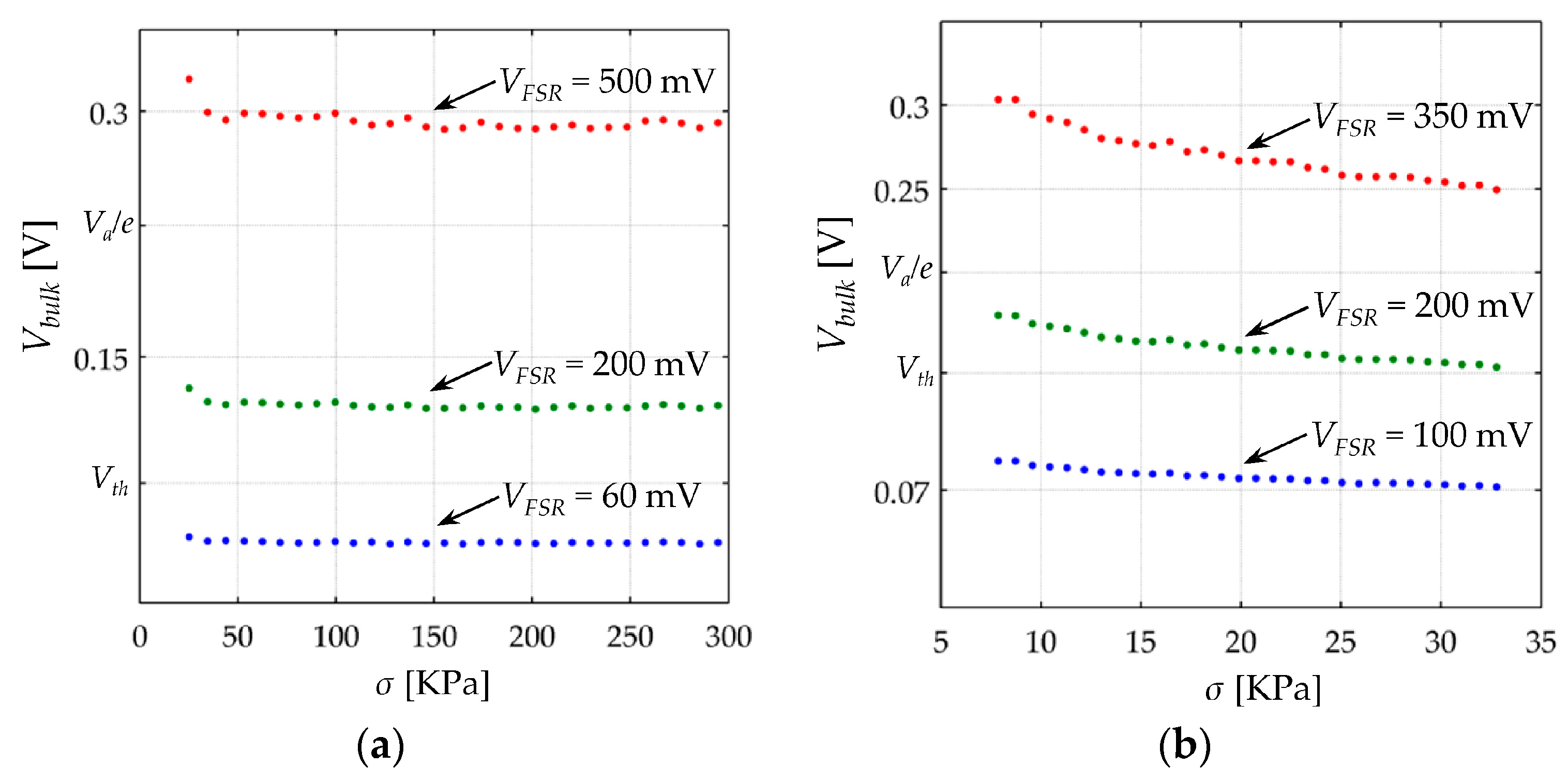
In a typical force sensing application,
VFSR is usually within the range (300 mV–5 V) [
13,
28]. It is later demonstrated in
Section 5 that under such circumstances, the value of
Vbulk is typically larger than
Va/e, and thus, Equation (8) can be taken as the equation for describing the current conduction in the polymer composite. Note that a close form for
Rbulk is not possible in such interval and only an
I-VFSR relationship can be formulated. When
VFSR is within the range (0 V–150 mV),
Rbulk has an ohmic behavior because
Vbulk is typically lower than
Vth. Thus, a close form for
Rbulk is possible in this interval. Finally, when
VFSR is within the range (150 mV–300 mV)
Vbulk is greater than
Vth but smaller than
Va/e, under such circumstances, Equation (7) describes the
I-VFSR relationship of the polymer composite.
Unfortunately, the previously mentioned intervals are approximated because Vbulk is a function of VFSR and Rc, see Equation (28). Hence, absolute intervals cannot be defined for Vbulk because Rc varies from one sensor to another, i.e., there are not two identical sensors. For such reason, the piecewise model for the polymer composite must be stated in terms of: Vbulk = VFSR − 2·I·Rc.
If
VFSR − 2·
I·
Rc <
Vth Equations (6), (16), (29), (30), (A2) and (A3) are combined as next:
where Equation (31) is valid only when
VFSR is approximately within the range (0 V–150 mV).
If
Vth
< VFSR − 2·
I·
Rc <
Va/e Equations (7), (16), (29), (30) and (A2) are combined as next:
where Equation (32) is valid only when
VFSR is approximately within the range (150 mV–300 mV)
Finally, if
VFSR − 2·
I·
Rc >
Va/e Equations (8), (16), (29), (30) and (A2) are combined as next:
where Equation (33) is valid only when
VFSR is greater than 300 mV.
Note that Equations (31)–(33) notably vary from the models previously described on
Section 3. The Equations (31)–(33) impose a voltage-dependent and area-dependent behavior for the current flowing through the polymer composite. Likewise, they do not rely upon experimental measurements of the electrical resistance at rest state,
R0.
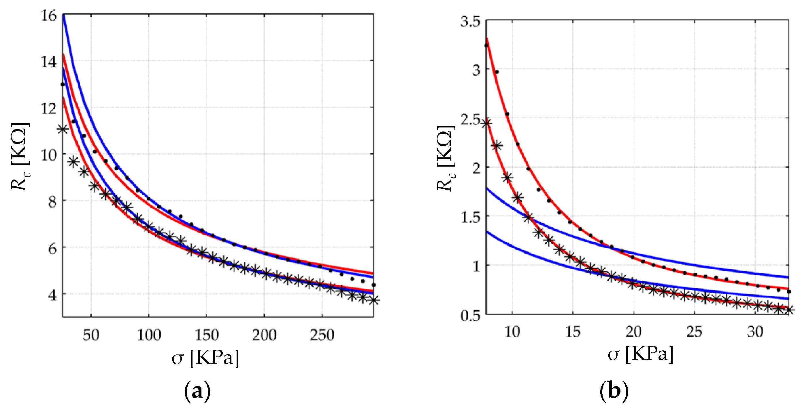
4.2. New Proposed Model for the Contact Resistance (Rc)
In
Section 2.3, a model for the contact resistance was presented based upon previous results from Kalantari et al. [
9]. Equation (11) predicts a reduction in the contact resistance in an inverse square root fashion of the applied force. However, as later demonstrated in
Section 5, the application of such a model is not suitable, at least for the FlexiForce and Interlink sensors. For this reason, the following model is proposed:
Previous Equation can be stated in terms of the applied force,
F, to allow comparison with the formulation from Kalantari et al.:
where
AFSR is the physical area of the FSR, and
is the value of the contact resistance at rest state.
Note from Equations (34) and (35) that an infinite resistance is expected when σ = F = 0. In practice, it does not occur because the sensor is preloaded with a small force imposed by the sensor encapsulating material which is tightly bonded around the sensor edges. An offset can be added to Equations (34) and (35) in the form of σ + σ0 or F + F0, but typically, the values of σ0 and F0 are negligible when compared with the exerted forces, so, they have not been included in the aforementioned equations.
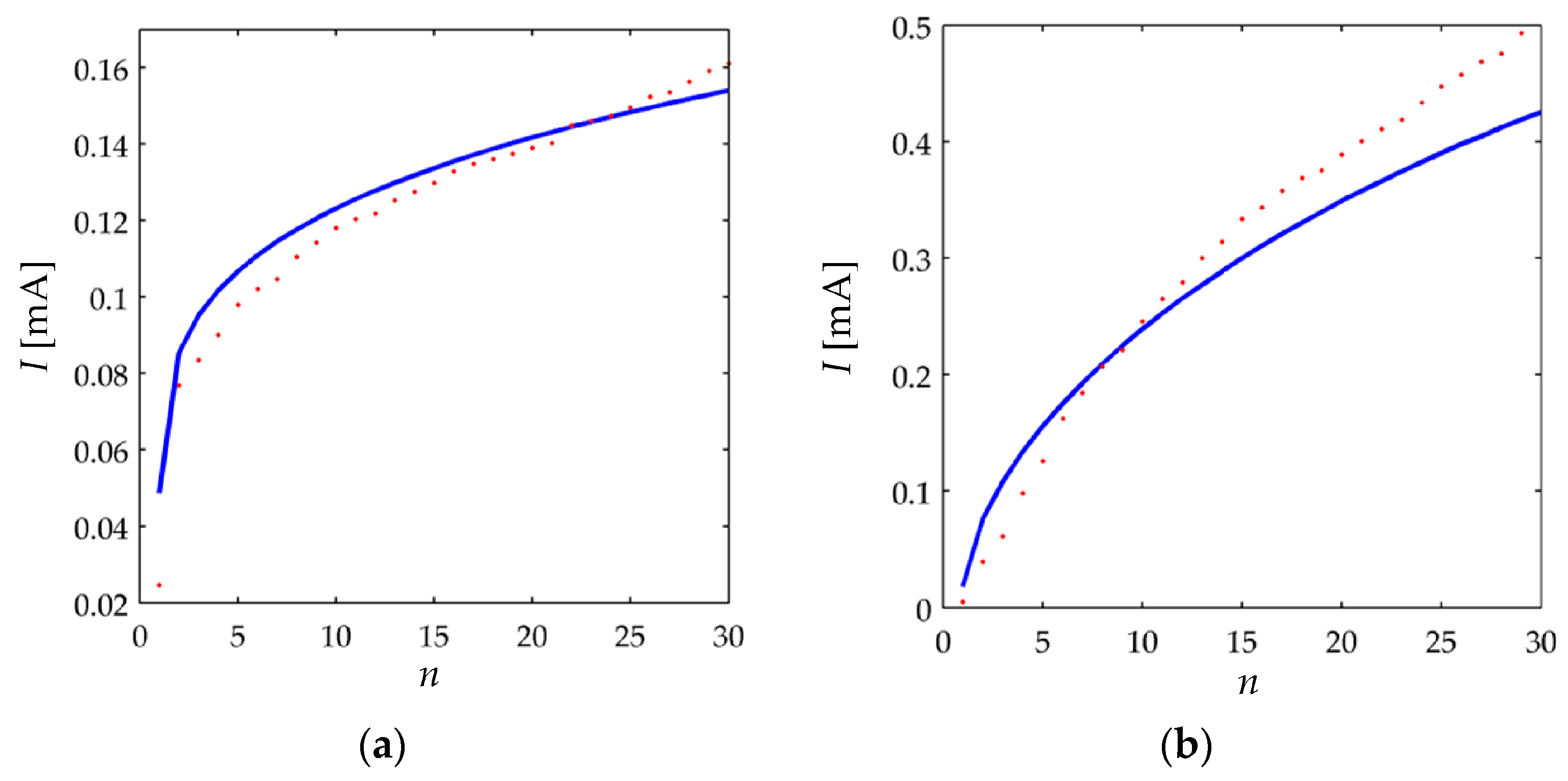
The resistance of the conductive particles,
Rpar, is included in Equations (34) and (35) because at the nano- and microscopic levels, the conductive particles behave as quantum point contacts, and thus, the classical definition of resistivity does not hold. This occurs when the length of the particle is comparable with 2π/
Kf, where
Kf is the Fermi wavefactor. Under such circumstances, the conductance of a nanoparticle is quantized in terms of the conductance quantum
G0:
The conductance increments occur in integer multiples of the particle length (
Lpar) as next:
where
n = 0, 1, 2… and
Kf is given by:
with
Ef standing for the Fermi energy of the particle. The phenomenon of quantum point contacts was discovered by independent studies carried out by Van Wees et al. [
39] and Wharam et al. [
40], but a comprehensive explanation of the phenomenon is addressed by Timp [
41]. In brief, for discrete increments of
Lpar, the particle’s conductance grows in a discrete fashion of
n·
G0. Only for sufficiently large values of
n, the conductance follows a continuous-classical-variation.
To the best of authors’ knowledge, the proposal of quantum point contacts for the conductive nanoparticles has not been considered before by any author in the polymer composite field [
33,
34,
42,
43,
44]. This is an important contribution since it complements previous models from Zhang et al. [
22], Wang et al. [
23] and Kalantari et al. [
9] in which they assumed that
Rpar is negligible when compared to
Rpol, see Equation (13). Moreover, the experimental results from
Section 5 support the hypothesis that
Rpar cannot be neglected.
On the other hand, the form
from Equation (34) and
from Equation (35) have been previously reported for the constriction (contact) resistance of materials with different sizes. In general, the constriction resistance follows power-laws as stated by Shi et al. [
45] and Mikrajuddin et al. [
36]. So, the form of Equations (34) and (35) is plausible as it models the series connection between the contact resistance—following power-laws—and the nanoparticle resistance. As previously stated, the underlying basis for the contact resistance can be found on the plastic and elastic interactions occurring between the conductive particles and the sensor electrodes at a microscopic level [
35]. Similarly, the increment in the effective area,
A, follows a power-law function as previously presented on Equations (29) and (30); this is not a coincidence as the behavior of
Rc and
A are tightly related, see
Section 2.3 and
Figure 6.
In
Section 5.2.1, experimental data are fitted to Equation (34) with good results. However, the model for the contact resistance can be further generalized, because as previously stated in Equation (12) the resistance of the conductive particles is computed from
L·
Rpar/
S, where
L and
S are the number of series-connected and parallel-connected particles, respectively. Nonetheless, when the applied stress increases more current paths are formed, and therefore, the number of parallel-connected particles,
S, also grows. This implies that
S should have the form
S(
σ), but for simplification purposes and considering the good results obtained, the proposed model from Equation (34) is henceforth used when modelling the contact resistance.
Finally, note that Equations (34) and (35) predict a voltage independent behavior for the contact resistance. This statement is experimentally demonstrated on
Section 5 on the basis of applying large values of
VFSR at different stresses.
4.3. Final Proposed Model for the I-VFSR Relationship of Force Sensing Resistors, FSRs
The final proposed model for the I-VFSR relationship of FSRs is based on combining the expression for the I-VFSR relationship of polymer composites, Equations (31)–(33), with the expression for the contact resistance.
For the sake of providing a consistent formulation with previous sections on this article, the final model is stated in terms of stress; hence Equation (34) is chosen as the mathematical expression for the contact resistance. The framework for combining both expressions is based upon Equations (27) and (28).
Considering that multiple symbols are embraced in the proposed model,
Table 1 summarizes the symbols employed by the authors while providing a comparison with previous notation from Zhang et al. [
22], Wang et al. [
23] and Kalantari et al. [
9]. The proposed model is presented next using piecewise functions in regard of
Vbulk, where
Vbulk =
VFSR − 2·
I·
Rc according to Equation (28).
If
VFSR − 2·
I·
Rc <
Vth, Equations (27), (31) and (34) are combined to obtain:
If
Vth
< VFSR − 2·
I·
Rc <
Va/e, Equations (28) and (32) are merged, so that
Vbulk is stated in terms of
VFSR and
Rc as next:
If
VFSR − 2·
I·
Rc >
Va/e, Equations (28) and (33) are merged, so that
Vbulk is stated in terms of
VFSR and
Rc as next:
where
Rc is given by Equation (34).
Equations (39)–(41) are stated in terms of the universal constants:
m,
e,
h, specific properties from the polymer and the nanoparticles:
s0,
M,
Va,
A0,
A1,
A2, and in terms of the contact resistance,
Rc. This last term can be independently estimated by re-arranging Equation (28):
For very large values of
VFSR, the
Vbulk term from Equation (42) can be set to 0 as an initial approximation because
I grows with the square of
Vbulk—see Equations (33) and (41)—whereas the voltage drop across the contact resistance,
VRc, grows linearly with the sensor current. This implies in practice, that for a constant stress, an increment in
VFSR—and hence on sensor current—yields a small increment of
Vbulk, whereas most of the additional
VFSR actually drops in the contact resistance, i.e., for large values of
VFSR,
Rc dominates because
Rbulk is diminished, see
Figure 4b. Finally, Equation (42) can be approximated to the following expression for sufficiently large values of
VFSR:
Equation (43) is very useful in practice because it allows an approximated estimation of the contact resistance in an empirical basis. Moreover, Equation (43) does not require information from the materials employed during the manufacturing process of the polymer composites. An iterative process that yields accurate results for Rc is addressed in the next Section.
6. Conclusions and Future Work
A model for the Current-Voltage relationship (I-VFSR) of Force Sensing Resistors (FSRs) and polymer composites has been derived and tested. The proposed model is capable of predicting sensor current based upon information from the applied stress, σ, and sourcing voltage, VFSR. This model exhibits multiple differences compared with previous contributions to the field, as it embraces three additional parameters which have been omitted or assumed constant by previous studies. These are: the non-linear I-VFSR relationship, the force-dependent behavior of the effective area for current conduction (A), and the resistance of the conductive particles (Rpar) deposited in the insulating polymer; such particles behave as quantum point contacts with nonzero resistance. Experimental evidence supports the force-dependent behavior of A, and similarly, the nonlinear I-VFSR relationship has been experimentally identified by applying different voltages at constant mechanical stress.
The proposed model has been implicitly formulated by using piecewise functions. It was obtained from a combination of two concepts from quantum mechanics and one concept from classical physics. The quantum concepts are: the tunneling conduction and the resistance of quantum point contacts. The pressure dependence on the contact resistance (Rc) of materials is the classical concept included in the model.
The proposed model was tested over commercially available FSRs manufactured by Interlink Electronics, Inc and Tekscan, Inc. In general, the test results are satisfactory, especially for the contact resistance, Rc. However, when modeling the tunneling conduction, a lower goodness of fit was obtained; this occurred because the literature regarding tunneling conduction was derived from a semi-classical solution for the Schrödinger equation (the WKB approximation), and due to the fact that numerical approximations were done by previous authors when deriving the I-VFSR relationship of thin insulating layers. Thus, one pending task is to derive a more accurate model for the current conduction of thin insulating film layers operating on the basis of quantum tunneling.
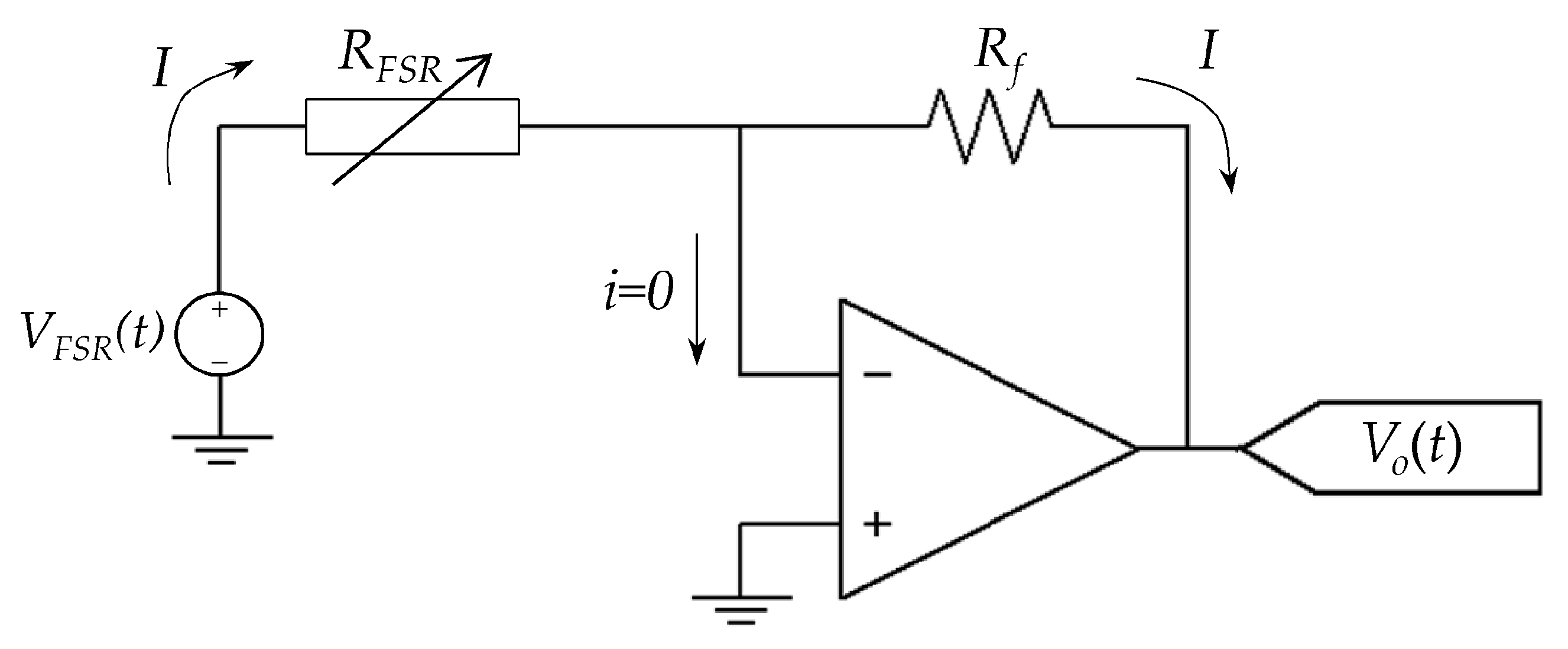
The authors discourage Wheatstone bridges, voltage dividers and multimeters as the experimental setup for reading the resistance of polymer composites (Rbulk) and FSRs (RFSR). Theoretical models and experimental evidence have been presented in this study in regard to the voltage-dependent behavior of Rbulk and RFSR. Wheatstone bridges, voltage dividers and multimeters operate on the basis of changing the voltage across the unknown resistance, and thus, a modulation effect is created as the applied stress and the applied voltage change simultaneously. Instead, authors encourage the usage of an amplifier in inverting configuration as the method to collect sensor data. Similarly, the voltage applied to the FSRs during testing, VFSR, should be specified by the authors in order to ensure the repeatability of results.
Future work possibilities are vast within the manufacturing and modeling of FSRs. From the manufacturing scope, the fabrication of FSRs using different materials and electrode configuration are research possibilities which are currently being explored by several authors. From the modeling standpoint, the inclusion of rheological models in the proposed model is currently a research focus of the authors; by doing this, creep compensation could be performed thus enhancing sensor performance. Similarly, the modeling and compensation of hysteresis are also being considered by the authors.


