Line-Constrained Camera Location Estimation in Multi-Image Stereomatching

Abstract
:1. Introduction
1.1. The Benefits of Multiple Views
1.2. The Importance of Camera Location Estimation
1.3. Outline
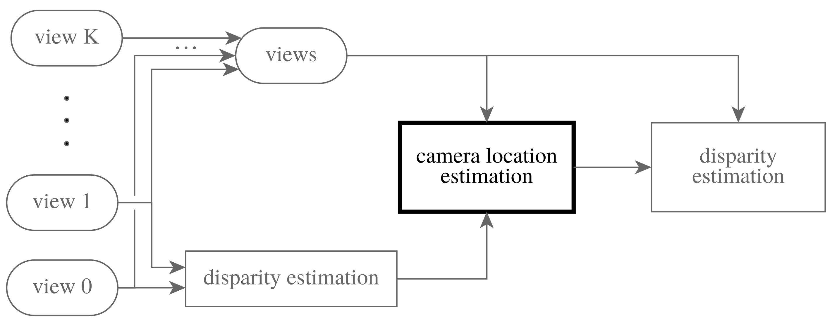
2. Methods
2.1. Multi-Image Stereomatching
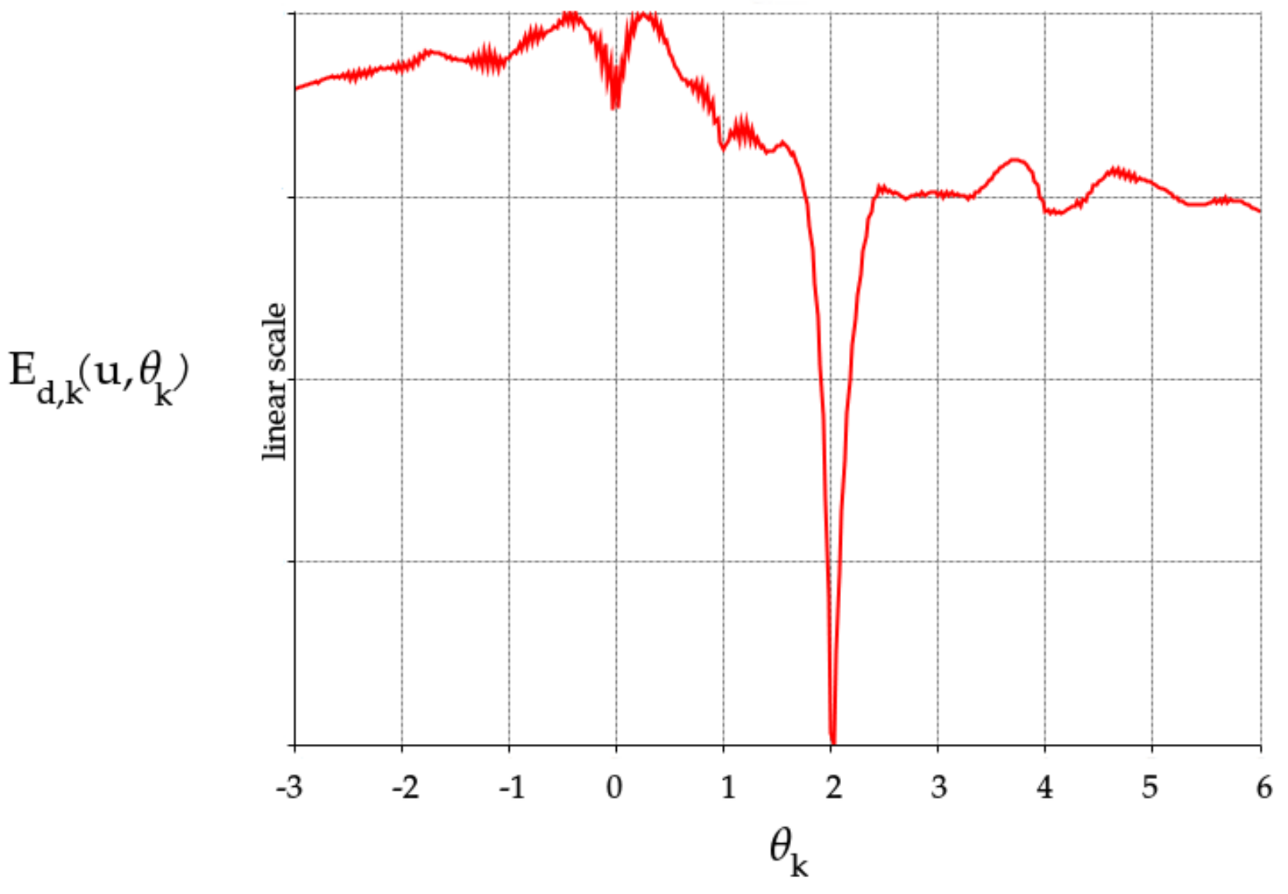
2.2. Camera Location Estimation
2.3. Monotonicity Constraint
2.4. Hierarchical Approach
2.5. Overview of the Entire Work Flow
| Algorithm 1: Overview of the proposed approach |
| u← disparity estimate from two views |
| for t from T-1 to 0 do |
| upscale by factor (bilinear) |
| resize by factor |
| for warp from 1 to W do |
| for ℓ from 1 to L do |
| the solution of the system Equation (9) (see Appendix A) |
| end for |
| end for |
| end for |
| u← disparity estimate from all views as described in [16]. |
- levels in the pyramid, with a scaling factor of ;
- warps per level;
- block-coordinate descent iterations per warp for optimizing the dual variables.
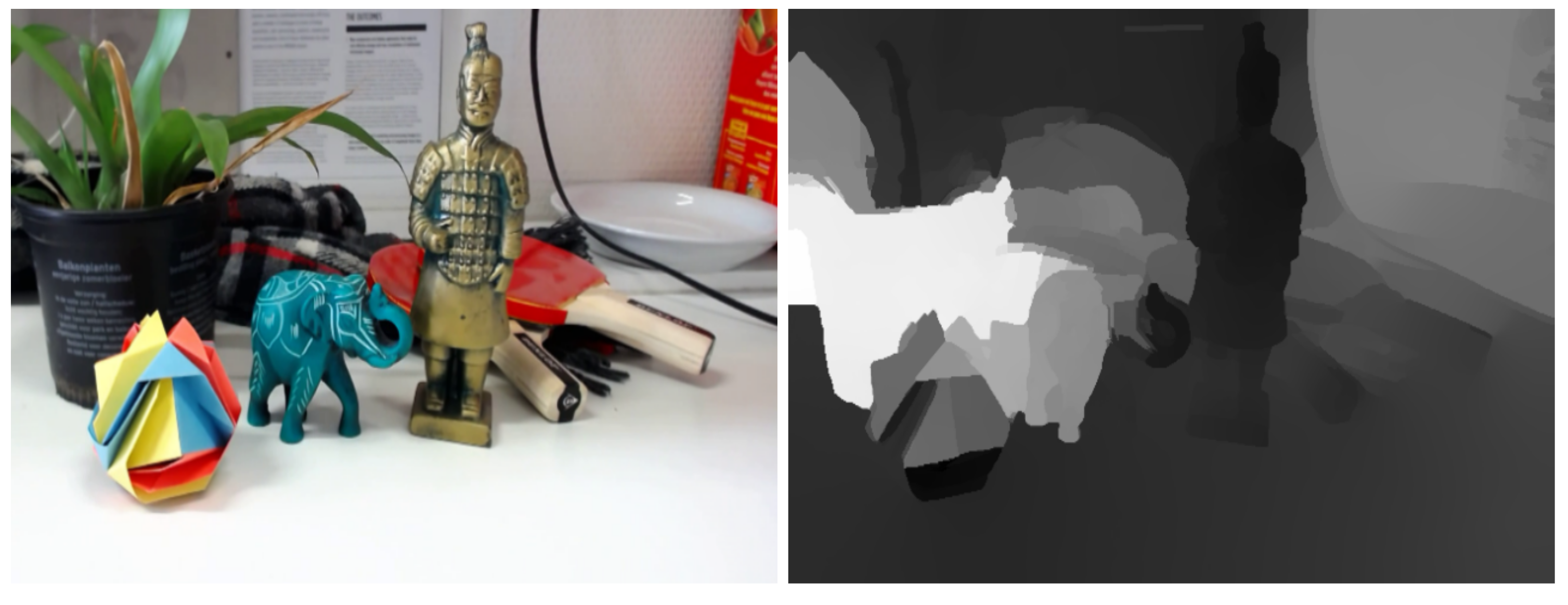
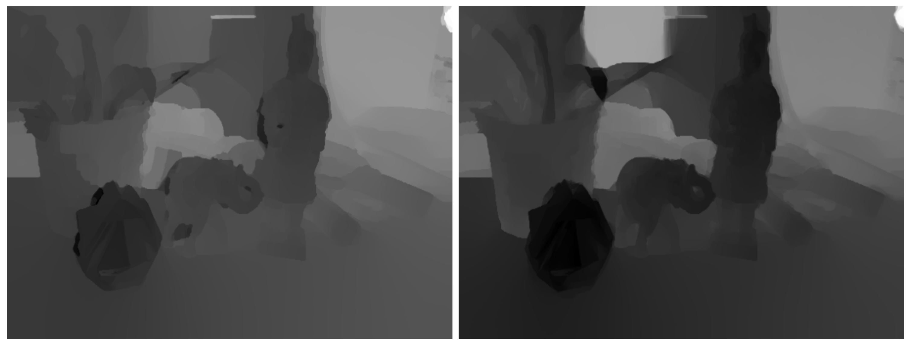
3. Results
3.1. Monotonicity Constraint
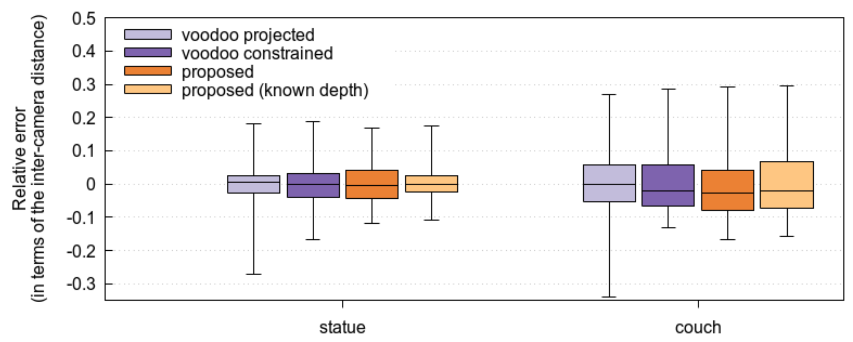
3.2. Accuracy of the Proposed Method
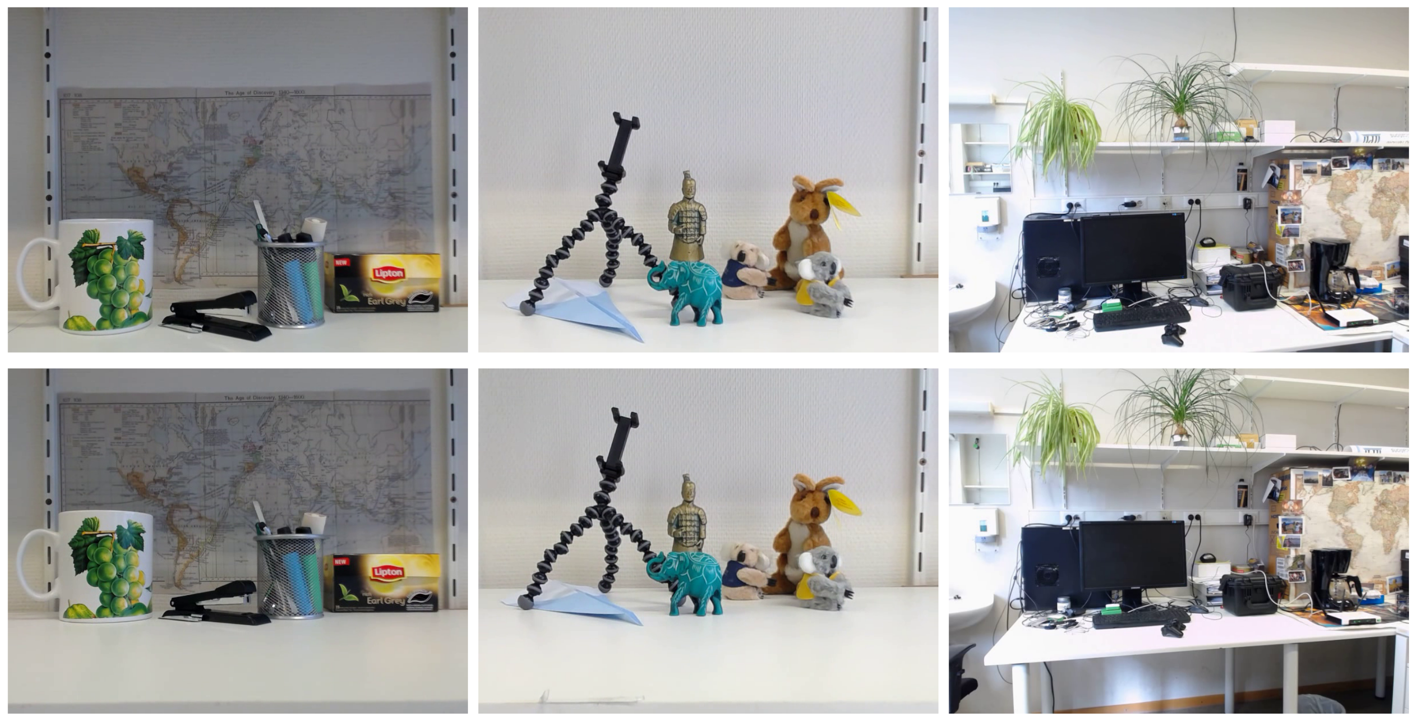
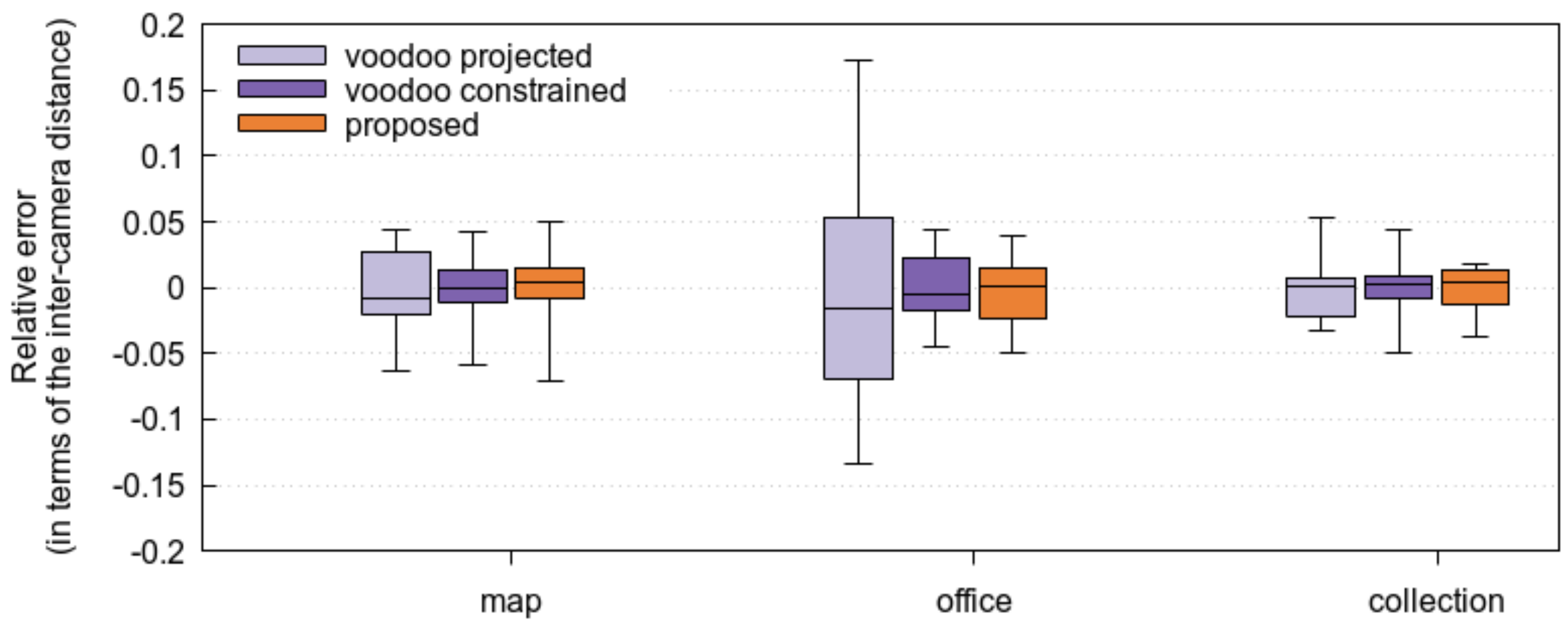
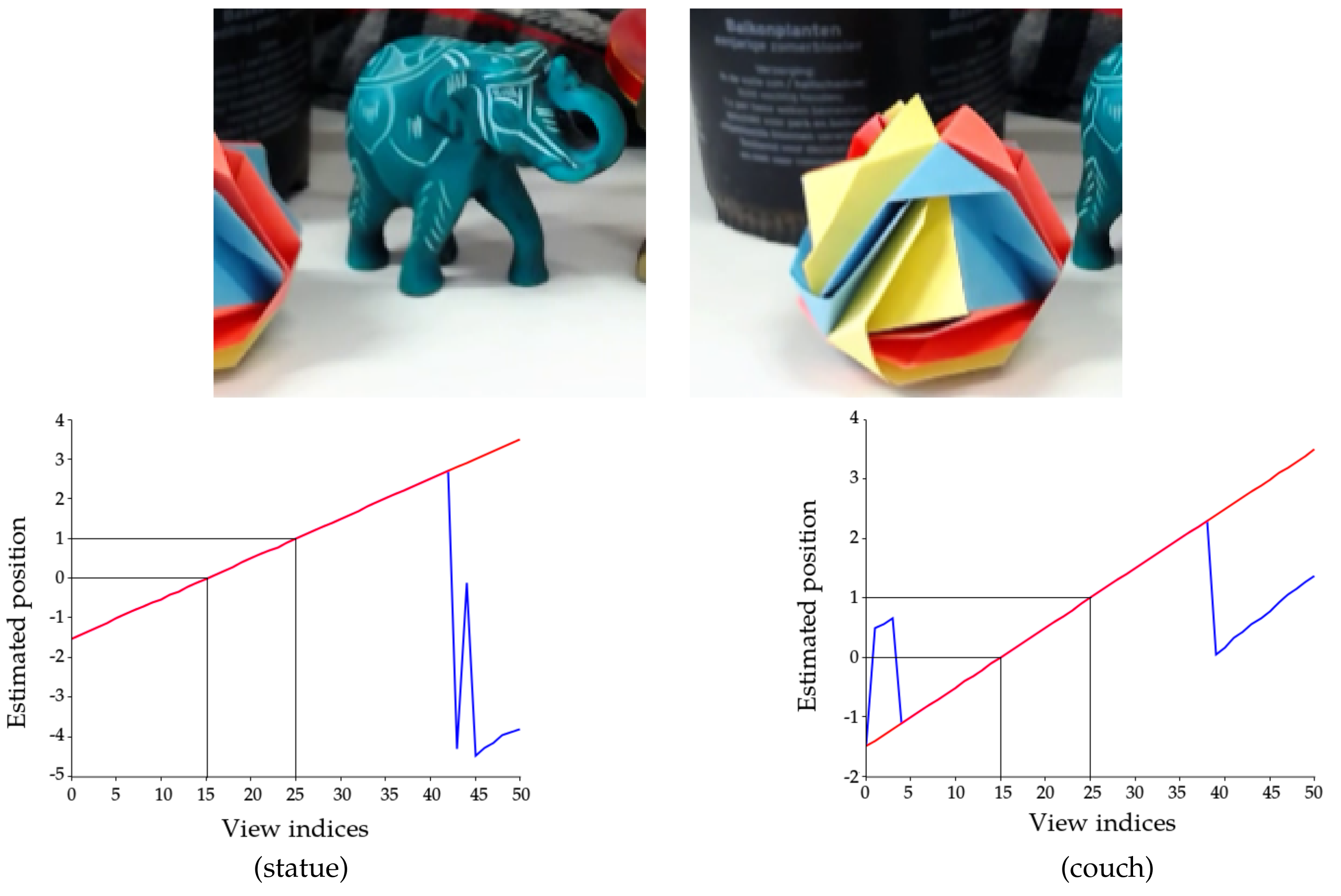
3.3. Estimation in a Practical Setting
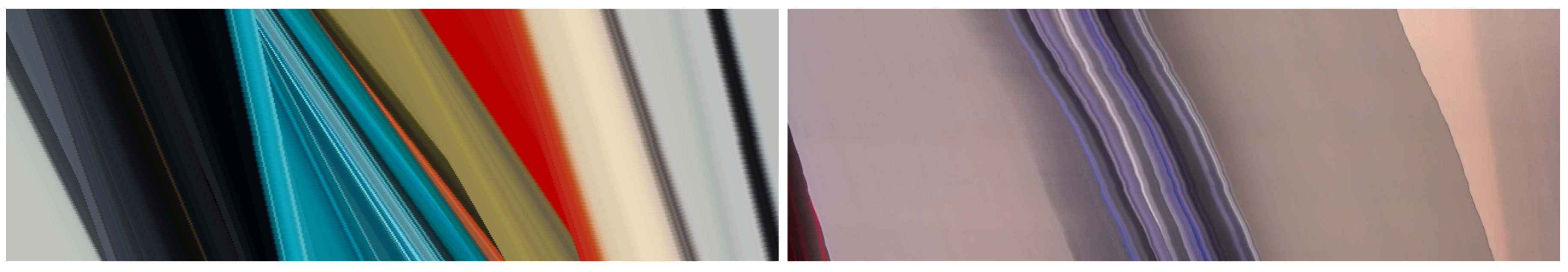
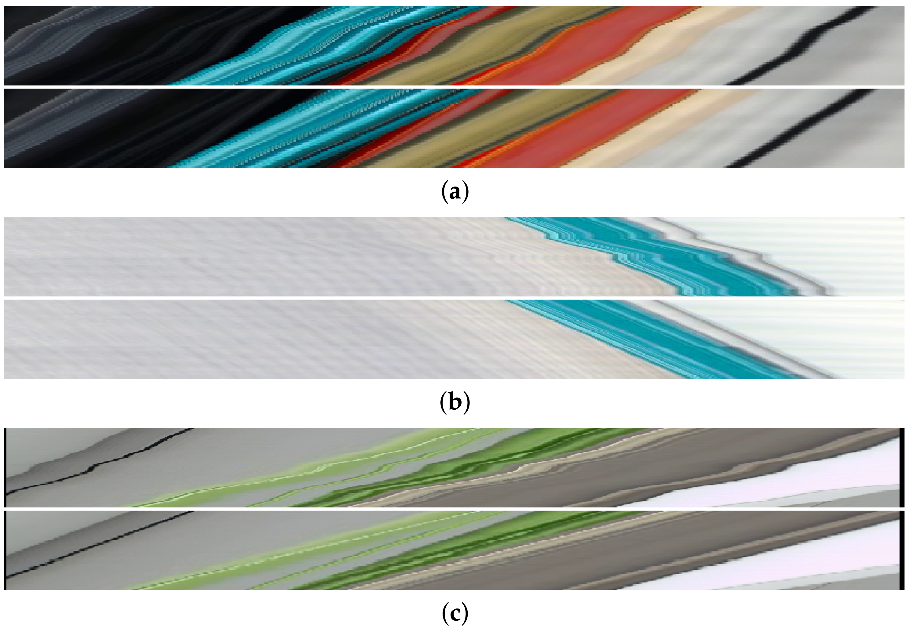
3.4. Rectifying the Epipolar Plane Images
4. Conclusions
Acknowledgments
Author Contributions
Conflicts of Interest
Appendix A. Deriving the Update Rules
Appendix B. Optimizing the Location Reference System for the Trackers
References
- Horn, B.K.; Schunck, B.G. Determining optical flow. Artif. Intell. 1981, 17, 319–331. [Google Scholar] [CrossRef]
- Gilliam, C.; Blu, T. Local All-Pass filters for optical flow estimation. In Proceedings of the IEEE International Conference on Acoustics, Speech and Signal Processing, Brisbane, QLD, Australia, 19–24 April 2015; pp. 1533–1537. [Google Scholar]
- Drulea, M.; Nedevschi, S. Motion Estimation Using the Correlation Transform. IEEE Trans. Image Process. 2013, 22, 3260–3270. [Google Scholar] [CrossRef] [PubMed]
- Richardt, C.; Orr, D.; Davies, I.; Criminisi, A.; Dodgson, N.A. Real-time spatiotemporal stereo matching using the dual-cross-bilateral grid. In Proceedings of the European Conference on Computer Vision, Crete, Greece, 5–11 September 2010; pp. 510–523. [Google Scholar]
- Ranftl, R.; Gehrig, S.; Pock, T.; Bischof, H. Pushing the limits of stereo using variational stereo estimation. In Proceedings of the IEEE Intelligent Vehicles Symposium, Alcala de Henares, Spain, 3–7 June 2012; pp. 401–407. [Google Scholar]
- Xu, L.; Jia, J.; Matsushita, Y. Motion Detail Preserving Optical Flow Estimation. IEEE Trans. Pattern Anal. Mach. Intell. 2012, 34, 1744–1757. [Google Scholar] [PubMed]
- Kennedy, R.; Taylor, C.J. Optical flow with geometric occlusion estimation and fusion of multiple frames. In Energy Minimization Methods in Computer Vision and Pattern Recognition; Springer: Berlin/Heidelberg, Germany, 2015; pp. 364–377. [Google Scholar]
- Braux-Zin, J.; Dupont, R.; Bartoli, A. A General Dense Image Matching Framework Combining Direct and Feature-Based Costs. In Proceedings of the International Conference on Computer Vision, Sydney, NSW, Australia, 1–8 December 2013; pp. 185–192. [Google Scholar]
- Gay-Bellile, V.; Bartoli, A.; Sayd, P. Direct Estimation of Nonrigid Registrations with Image-Based Self-Occlusion Reasoning. IEEE Trans. Pattern Anal. Mach. Intell. 2010, 32, 87–104. [Google Scholar] [CrossRef] [PubMed]
- Zhang, L.; Zhang, K.; Chang, T.S.; Lafruit, G.; Kuzmanov, G.K.; Verkest, D. Real-Time High-Definition Stereo Matching on FPGA. In Proceedings of the 19th ACM/SIGDA International Symposium on Field Programmable Gate Arrays, Monterey, CA, USA, 27 February–1 March 2011; pp. 55–64. [Google Scholar]
- Chambolle, A.; Pock, T. A First-Order Primal-Dual Algorithm for Convex Problems with Applications to Imaging. J. Math. Imaging Vis. 2011, 40, 120–145. [Google Scholar] [CrossRef]
- Sun, J.; Zheng, N.N.; Shum, H.Y. Stereo matching using belief propagation. IEEE Trans. Pattern Anal. Mach. Intell. 2003, 25, 787–800. [Google Scholar]
- Wanner, S.; Meister, S.; Goldluecke, B. Datasets and Benchmarks for Densely Sampled 4D Light Fields. In Annual Workshop on Vision, Modeling & Visualization; The Eurographics Association: Geneva, Switzerland, 2013; pp. 225–226. [Google Scholar]
- Heber, S.; Ranftl, R.; Pock, T. Variational Shape from Light Field. In Energy Minimization Methods in Computer Vision and Pattern Recognition; Springer: Berlin/Heidelberg, Germany, 2013; pp. 66–79. [Google Scholar]
- Kim, C.; Zimmer, H.; Pritch, Y.; Sorkine-Hornung, A.; Gross, M. Scene Reconstruction from High Spatio-angular Resolution Light Fields. ACM Trans. Graph. 2013, 32, 73. [Google Scholar] [CrossRef]
- Donné, S.; Goossens, B.; Aelterman, J.; Philips, W. Variational Multi-Image Stereo Matching. Proceedings of IEEE International Conference on Image Processing, Quebec City, QC, Canada, 27–30 September 2015; pp. 897–901. [Google Scholar]
- Oram, D. Rectification for any epipolar geometry. BMVC 2001, 1, 653–662. [Google Scholar]
- Fusiello, A.; Irsara, L. Quasi-Euclidean uncalibrated epipolar rectification. In Proceedings of the 19th International Conference on IEEE Pattern Recognition (ICPR), Tampa, FL, USA, 8–11 December 2008; pp. 1–4. [Google Scholar]
- Levoy, M.; Hanrahan, P. Light Field Rendering. In Proceedings of the 23rd Annual Conference on Computer Graphics and Interactive Techniques, New Orleans, LA, USA, 4–9 August 1996; pp. 31–42. [Google Scholar]
- Adelson, E.; Wang, J. Single lens stereo with a plenoptic camera. IEEE Trans. Pattern Anal. Mach. Intell. 1992, 14, 99–106. [Google Scholar] [CrossRef]
- Voodoo Camera Tracker. Available online: http://www.viscoda.com (accessed on 17 August 2017).
- Hartley, R.; Zisserman, A. Multiple View Geometry in Computer Vision; Cambridge University Press: Cambridge, UK, 2003. [Google Scholar]
- Kahl, F.; Hartley, R. Multiple-View Geometry Under the L∞-Norm. IEEE Trans. Pattern Anal. Mach. Intell. 2008, 30, 1603–1617. [Google Scholar] [CrossRef] [PubMed]
- Olsson, C.; Eriksson, A.P.; Kahl, F. Efficient optimization for L∞ problems using pseudoconvexity. In Proceedings of the 2007 IEEE 11th International Conference on Computer Vision, Rio de Janeiro, Brazil, 14–21 October 2007; pp. 1–8. [Google Scholar]
- Goossens, B.; De Vylder, J.; Philips, W. Quasar: A new heterogeneous programming framework for image and video processing algorithms on CPU and GPU. In Proceedings of the IEEE International Conference on Image Processing, Paris, France, 27–30 October 2014; pp. 2183–2185. [Google Scholar]
- Zabih, R.; Woodfill, J. Non-parametric local transforms for computing visual correspondence. In Proceedings of the European Conference on Computer Vision, Stockholm, Sweden, 2–6 May 1994; pp. 151–158. [Google Scholar]
- Hafner, D.; Demetz, O.; Weickert, J.; Reißel, M. Mathematical Foundations and Generalisations of the Census Transform for Robust Optic Flow Computation. J. Math. Imaging Vis. 2014, 52, 71–86. [Google Scholar] [CrossRef]
- Bailer, C.; Taetz, B.; Stricker, D. Flow Fields: Dense Correspondence Fields for Highly Accurate Large Displacement Optical Flow Estimation. In Proceedings of the IEEE International Conference on Computer Vision, Santiago, Chile, 7–13 December 2015; pp. 4015–4023. [Google Scholar]
- Kılıç, E. Explicit formula for the inverse of a tridiagonal matrix by backward continued fractions. Appl. Math. Comput. 2008, 197, 345–357. [Google Scholar] [CrossRef]
- Mallik, R.K. The inverse of a tridiagonal matrix. Linear Algebra Appl. 2001, 325, 109–139. [Google Scholar] [CrossRef]


© 2017 by the authors. Licensee MDPI, Basel, Switzerland. This article is an open access article distributed under the terms and conditions of the Creative Commons Attribution (CC BY) license (http://creativecommons.org/licenses/by/4.0/).
Share and Cite
Donné, S.; Goossens, B.; Philips, W. Line-Constrained Camera Location Estimation in Multi-Image Stereomatching. Sensors 2017, 17, 1939. https://doi.org/10.3390/s17091939
Donné S, Goossens B, Philips W. Line-Constrained Camera Location Estimation in Multi-Image Stereomatching. Sensors. 2017; 17(9):1939. https://doi.org/10.3390/s17091939
Chicago/Turabian StyleDonné, Simon, Bart Goossens, and Wilfried Philips. 2017. "Line-Constrained Camera Location Estimation in Multi-Image Stereomatching" Sensors 17, no. 9: 1939. https://doi.org/10.3390/s17091939
APA StyleDonné, S., Goossens, B., & Philips, W. (2017). Line-Constrained Camera Location Estimation in Multi-Image Stereomatching. Sensors, 17(9), 1939. https://doi.org/10.3390/s17091939