
Sea Ice Detection Based on an Improved Similarity Measurement Method Using Hyperspectral Data


Abstract
:1. Introduction
2. Improved Similarity Measurement Method
2.1. Pixel Selection
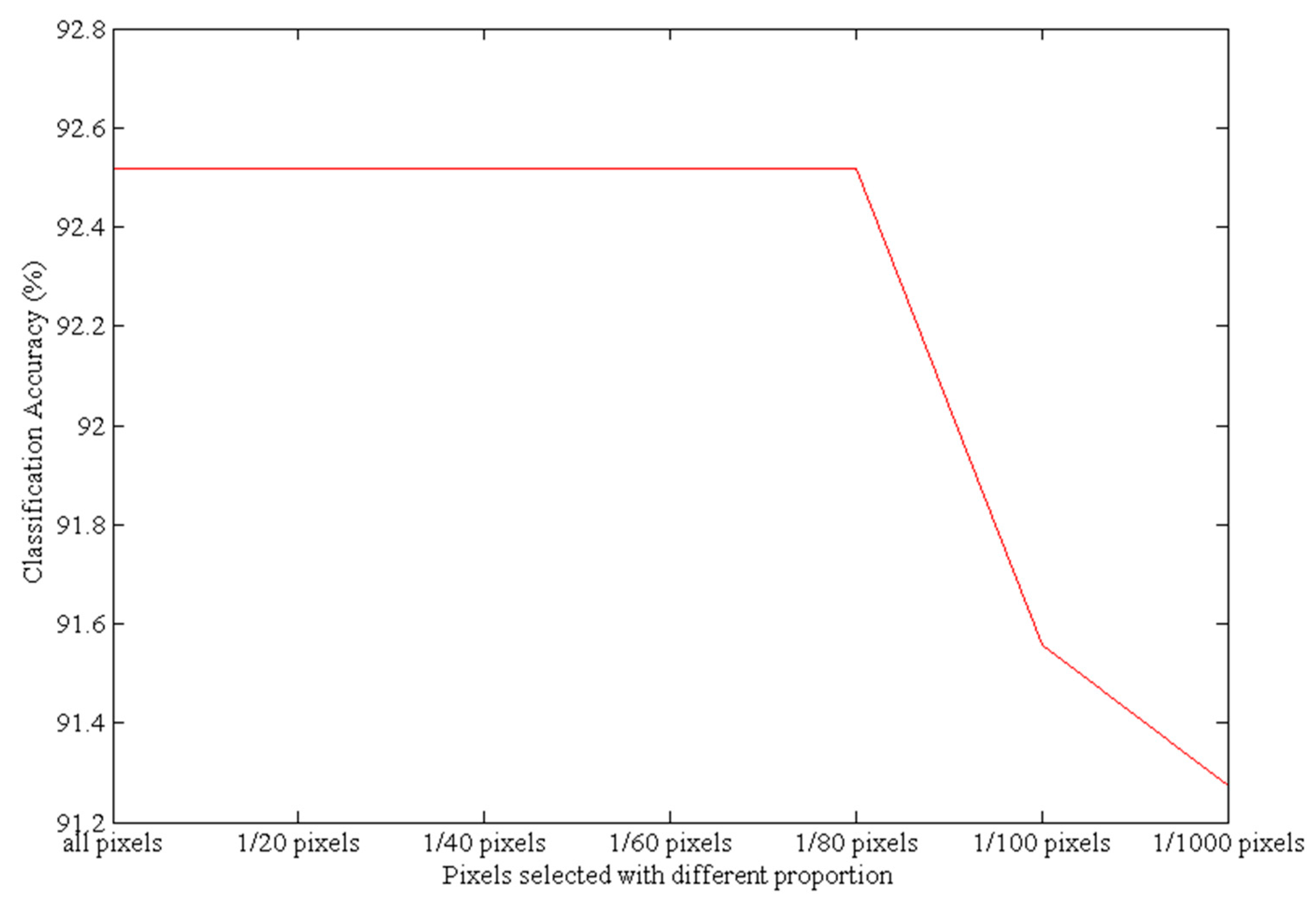
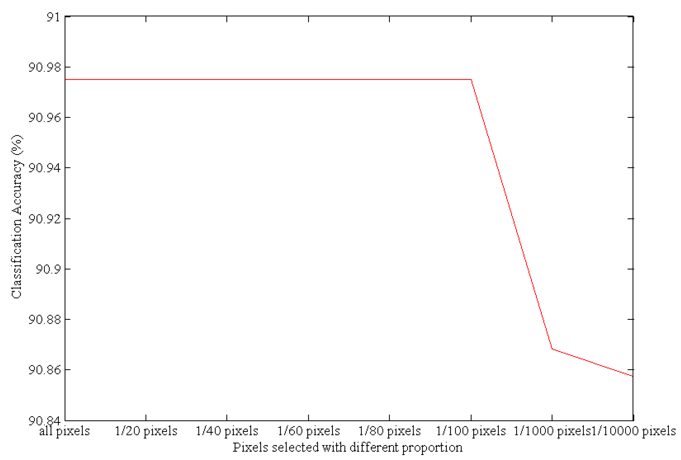
- Number of selected pixels: First select a band with all pixels, followed by a comparative analysis using all pixels, 1/100 pixels, 1/1000 pixels, 1/10,000 pixels, etc.
- Locations of the selected pixels: When using a low proportion to randomly select pixels for an entire image, not all categories of pixels can always be included in all cases. To eliminate this effect, this investigation adopted a pixel-selection method using K-means clustering. The specific steps are as follows:
- 1
- Select all the bands (after removing the invalid bands without radiometric calibration), perform the K-means clustering classification, and then merge the same categories.
- 2
- Calculate the number and locations of different categories of pixels, and determine the number of pixels in each category.
- 3
- According to step 2, choose the corresponding pixels in each type by uniform randomness.
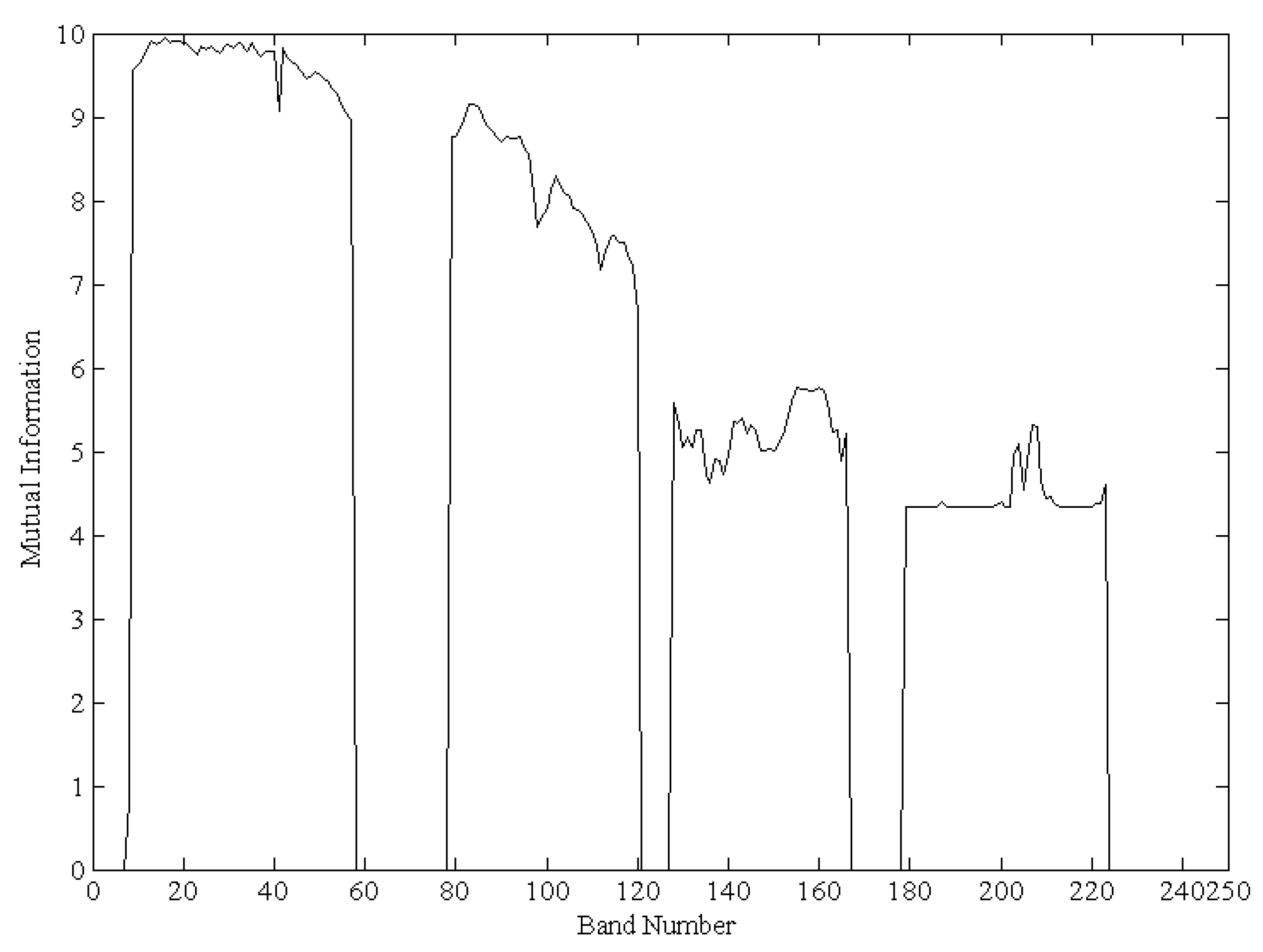
2.2. Band Selection Method
2.2.1. Original Band Selection Method
2.2.2. Subsequent Band Selection Method
- Initialize the algorithm with the pair B1 and B2, and construct a band subset Φ = {B1, B2}.
- Find B3, which is the band least similar to B1 and B2, and then update the selected band subset to .
- Repeat until the subset Φ contains a sufficient number of bands.
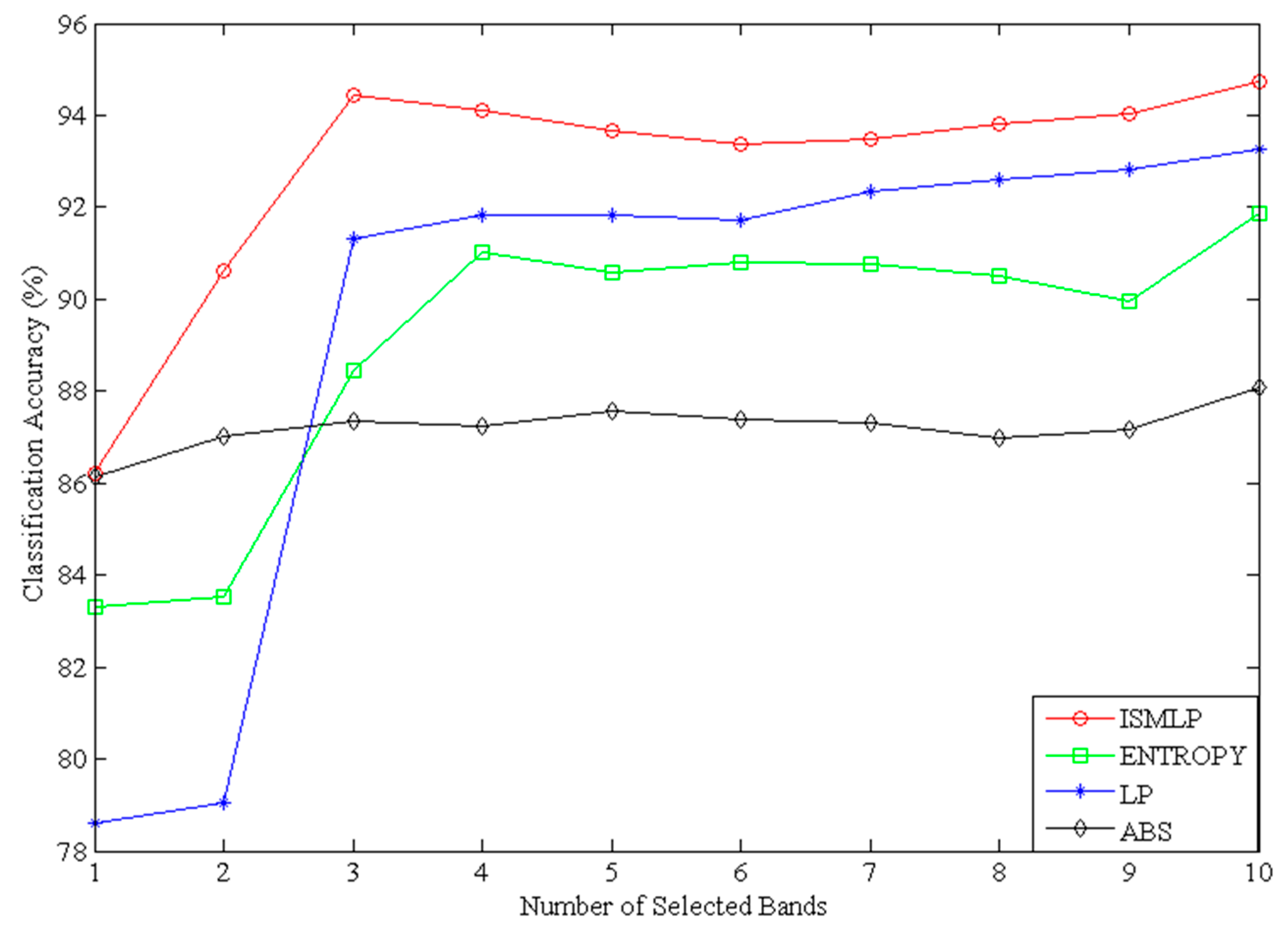
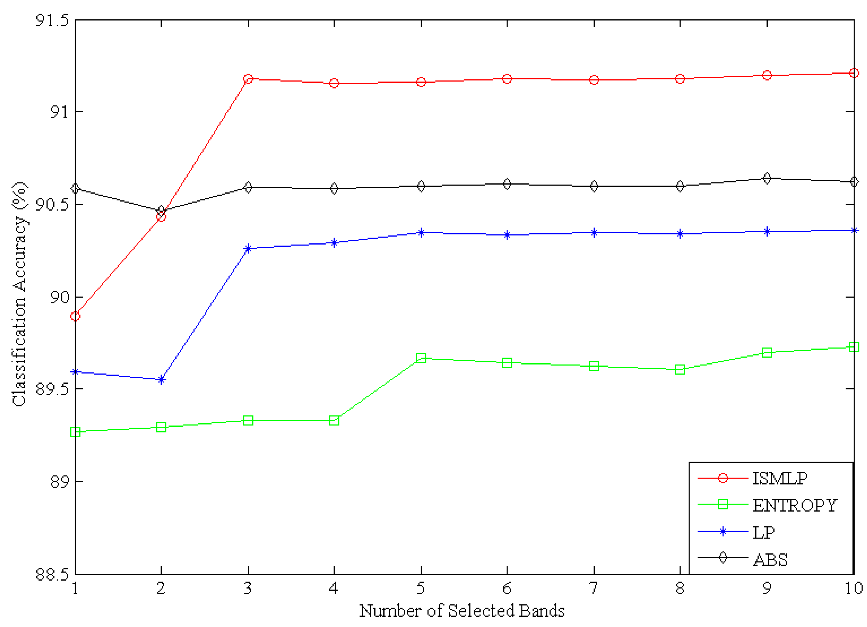
2.2.3. Number of Selected Bands
2.3. Sea Ice Classification Model
3. Experimental Analysis
3.1. Experiment in Baffin Bay
3.1.1. Data Description
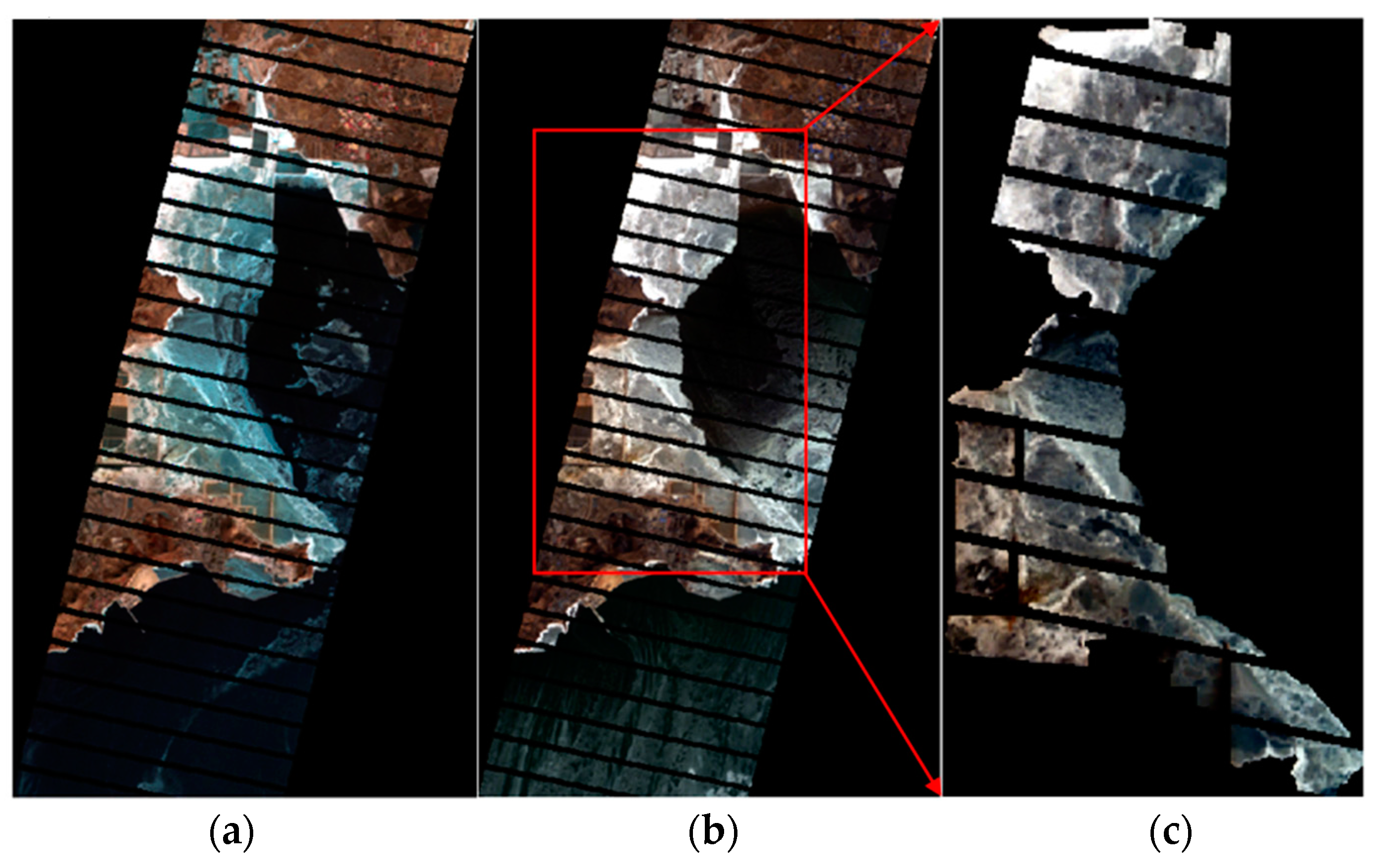
3.1.2. Preprocessing of Hyperspectral Data
3.1.3. Pixel Selection and Band Selection Based on the ISMLP Method
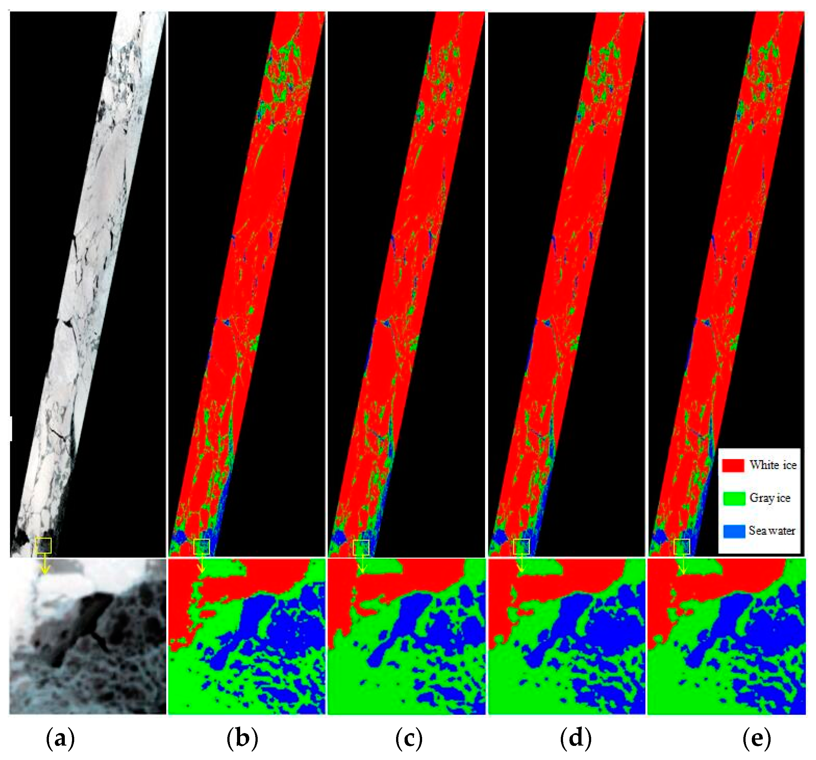
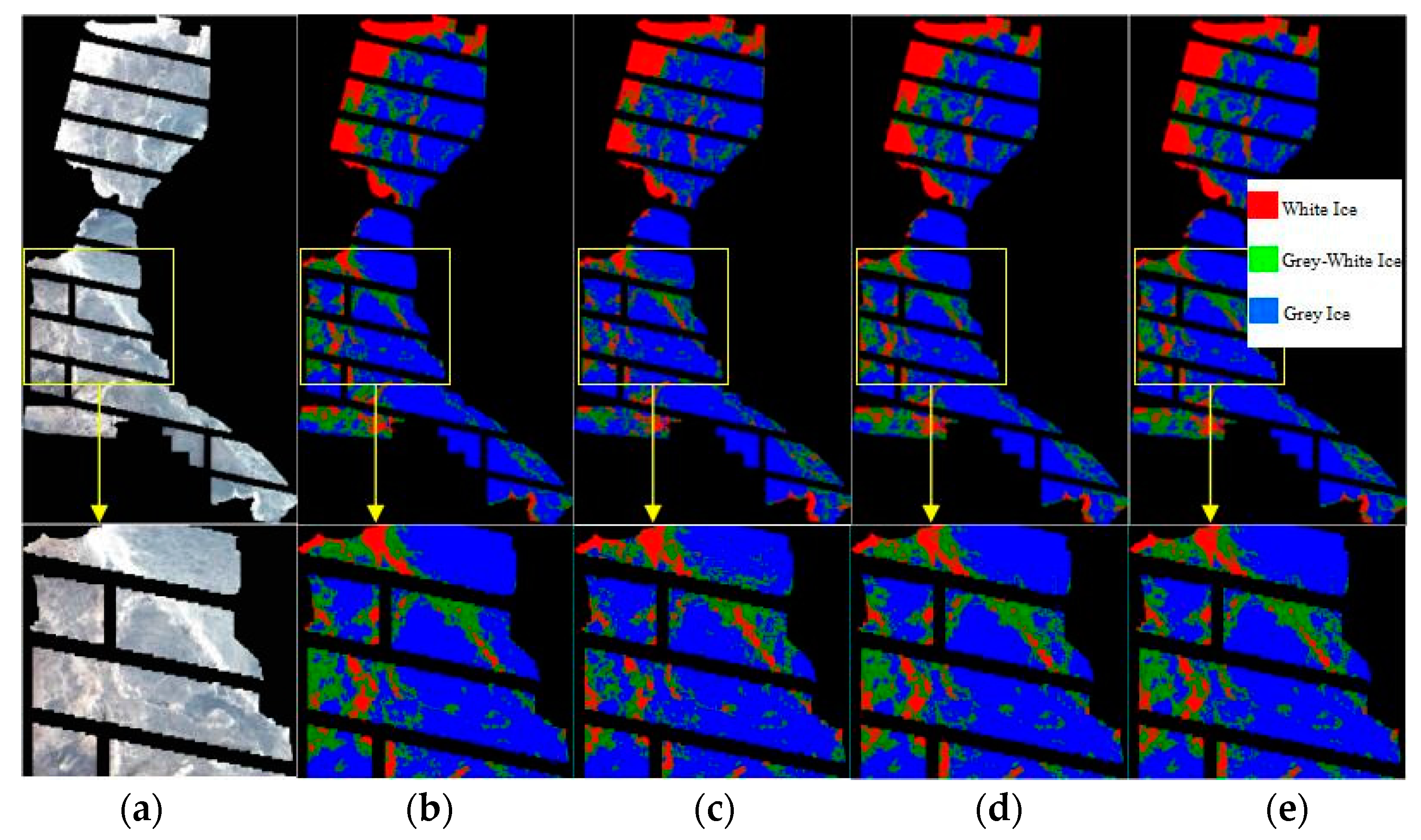
3.1.4. Accuracy Evaluation of the Sea Ice Detection Method
3.2. Experiment in Bohai Bay
3.2.1. Data Description
3.2.2. Preprocessing of Hyperspectral Data
3.2.3. Pixel Selection and Band Selection Based on the ISMLP Method
3.2.4. Accuracy Evaluation of Sea Ice Detection
4. Conclusions
- Considering each band’s information and the similarity between bands, the proposed ISMLP method produces the best classification accuracy compared to the traditional methods while also greatly reducing the data dimensions.
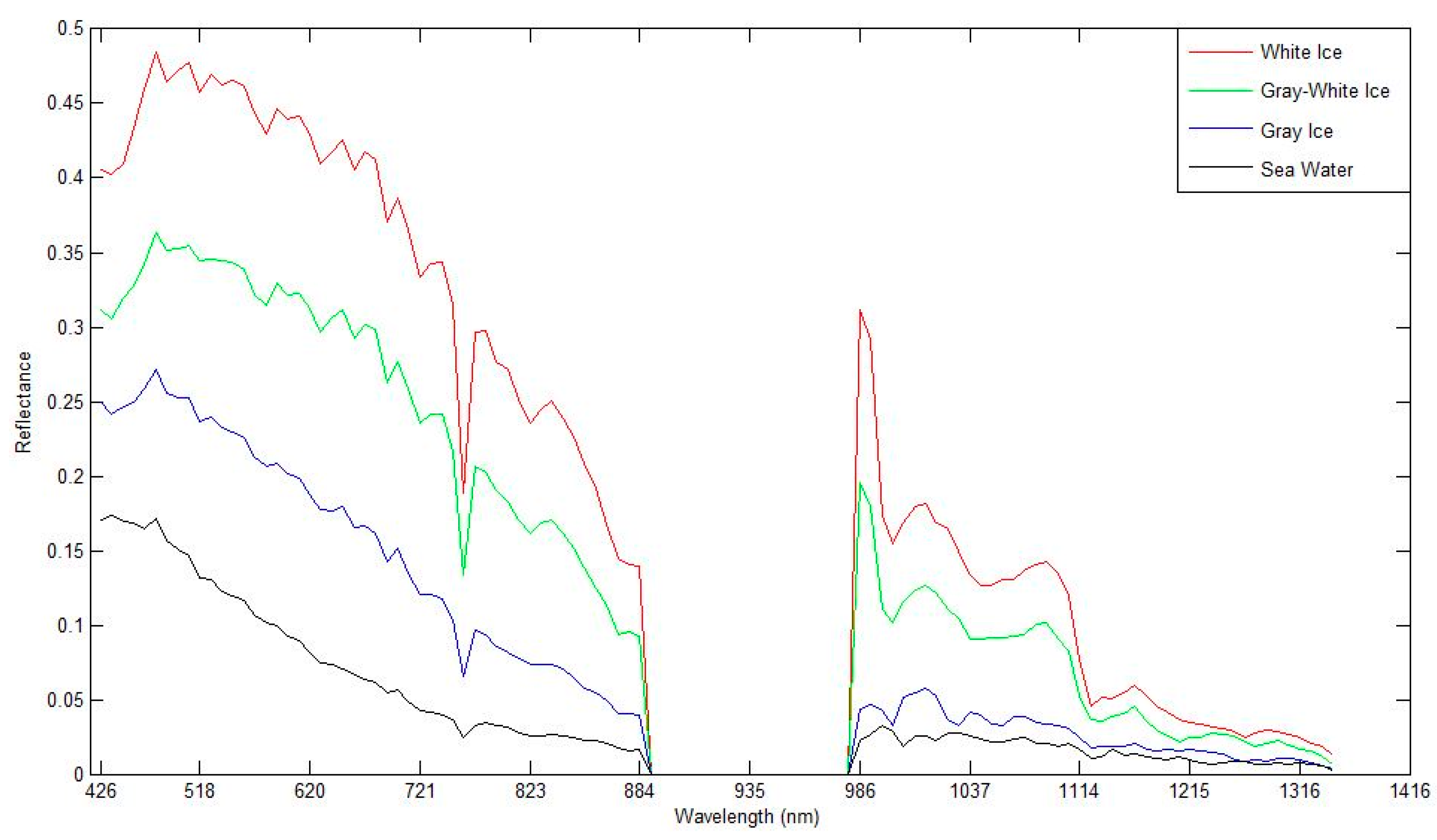
- Considering the spectral characteristics of sea ice, this work chose bands that have good spectral characteristics and separability and applied the band selection of the hyperspectral image to only those bands. This approach effectively reduces the scope of the original bands and enhances the efficiency of the method.
- Considering the high spatial correlations in the hyperspectral images, we selected pixels based on K-means clustering and analyzed the changes in the classification accuracy resulting from pixel selection at different proportions. The results revealed that selecting a proportion of approximately 1/100 pixels with K-means maintains the balance between efficiency and performance. That is, the 1/100 pixel-selection proportion reduced the computational cost while simultaneously achieving higher classification accuracy than other pixel-selection proportions.
Acknowledgments
Author Contributions
Conflicts of Interest
References
- Deser, C.; Walsh, J.E.; Timlin, M.S. Arctic sea ice variability in the context of recent atmospheric circulation trends. J. Clim. 2000, 13, 617–633. [Google Scholar] [CrossRef]
- Thomas, D.N. Sea Ice, 3rd ed.; Wiley-Blackwell: Hoboken, NJ, USA, 2017. [Google Scholar]
- Luo, Z.Y.; Sun, L. Study on Bohai seaice monitoring based on hyperspectral remote sensing imagery. Sci. Surv. Mapp. 2012, 37, 54–55. [Google Scholar]
- Laine, V. Antarctic ice sheet and sea ice regional albedo and temperature change, 1981–2000, from AVHRR Polar Pathfinder data. Remote Sens. Environ. 2008, 112, 646–667. [Google Scholar] [CrossRef]
- Hall, D.K.; Key, J.R.; Casey, K.A.; Riggs, G.A.; Cavalieri, D.J. Sea ice surface temperature product from MODIS. IEEE Trans. Geosci. Remote Sens. 2004, 42, 1076–1087. [Google Scholar] [CrossRef]
- Melgani, F.; Bruzzone, L. Classification of hyperspectral remote sensing images with support vector machines. IEEE Trans. Geosci. Remote Sens. 2004, 42, 1778–1790. [Google Scholar] [CrossRef]
- Xie, H.; Tong, X.H. A probability-based improved binary encoding algorithm for classification of hyperspectral images. IEEE J. Sel. Top. Appl. Earth Obs. Remote Sens. 2014, 7, 2108–2118. [Google Scholar] [CrossRef]
- Tong, X.H.; Xie, H.; Weng, Q. Urban land cover classification with airborne hyperspectral data: What features to use? IEEE J. Sel. Top. Appl. Earth Obs. Remote Sens. 2014, 7, 3998–4009. [Google Scholar] [CrossRef]
- Ke, C.Q.; Xie, H.J.; Lei, R.B.; Li, Q.; Sun, B. Spectral features analysis of sea ice in the Arctic ocean. Spectrosc. Spectr. Anal. 2012, 32, 1081–1084. [Google Scholar]
- Hughes, G. On the mean accuracy of statistical pattern recognizers. IEEE Trans. Inf. Theory 1968, 14, 55–63. [Google Scholar] [CrossRef]
- Yang, H.; Du, Q.; Su, H.; Sheng, Y. An efficient method for supervised hyperspectral band selection. IEEE Geosci. Remote Sens. Lett. 2011, 8, 138–142. [Google Scholar] [CrossRef]
- Fang, Q.; Liu, J. Novel face feature extraction method based on PCA/ICA. Electron. Meas. Technol. 2010, 33, 31–34. [Google Scholar]
- Wang, H.; Angelopoulou, E. Average Normalized Information: A Novel Entropy-Based Band Selection Method; Technical Report CS-2004-13; Stevens Institute Technology: Hoboken, NJ, USA, 2004. [Google Scholar]
- Du, Q.; Yang, H. Similarity-based unsupervised band selection for hyperspectral image analysis. IEEE Geosci. Remote Sens. Lett. 2008, 5, 564–568. [Google Scholar] [CrossRef]
- Yang, J.; Yin, Q.; Zhou, N. An improved method of hyperspectral remote sensing data adaptive band selection. Remote Sens. Technol. Appl. 2007, 22, 513–519. [Google Scholar]
- Bajcsy, P.; Groves, P. Methodology for hyperspectral band selection. Photogramm. Eng. Remote Sens. 2004, 70, 793–802. [Google Scholar] [CrossRef]
- Zhou, Y.; Li, X.; Zhao, L. Modified Linear-Prediction Based Band Selection for Hyperspectral Image. Acta Opt. Sin. 2013, 33, 0828002. [Google Scholar] [CrossRef]
- Conese, C.; Maselli, F. Selection of optimum bands from TM scenes through mutual information analysis. ISPRS J. Photogramm. Remote Sens. 1993, 48, 2–11. [Google Scholar] [CrossRef]
- Chen, J.; Jia, X.; Hong, Z.; Zhang, Y.; Zhang, L.; Meng, W.; Gu, Q. Generalization of subpixel analysis for hyperspectral data with flexibility in spectral similarity measures. IEEE Trans. Geosci. Remote Sens. 2009, 47, 2165–2171. [Google Scholar] [CrossRef]
- Han, Y.; Ren, J. Active Learning Algorithms for the Classification of Hyperspectral Sea Ice Images. Math. Probl. Eng. 2015. [Google Scholar] [CrossRef]
- Zhang, L.; Zhou, W.; Wu, C.; Huo, J.; Zou, H.; Jiao, L. Center matching scheme for K-means cluster ensembles. Int. Soc. Opt. Photonics 2009, 7496, 749614. [Google Scholar] [CrossRef]
- Guo, B.; Gunn, S.R.; Damper, R.I.; Nelson, J.D.B. Band selection for hyperspectral image classification using mutual information. IEEE Geosci. Remote Sens. Lett. 2006, 3, 522–526. [Google Scholar] [CrossRef]
- Ifarraguerri, A.; Prairie, M.W. Visual method for spectral band selection. IEEE Geosci. Remote Sens. Lett. 2004, 1, 101–106. [Google Scholar] [CrossRef]
- Chang, C.I.; Du, Q. Estimation of number of spectrally distinct signal sources in hyperspectral imagery. IEEE Trans. Geosci. Remote Sens. 2004, 42, 608–619. [Google Scholar] [CrossRef]
- Roger, R.E. Principal Components transform with simple, automatic noise adjustment. Int. J. Remote Sens. 1996, 17, 2719–2727. [Google Scholar] [CrossRef]
- Wu, Q.Y.; Meng, T.L.; Wu, S. Research progress of image thresholding methods in recent 20 years (1994–2014). J. Data Acquis. Process. 2015, 30, 1–23. [Google Scholar]
- Barry, P. EO-1/Hyperion Science Data User’s Guide, Level 1_B. TRW Space Def. Inf. Syst. 2001, 555–557. [Google Scholar]
- Hossain, M.S.; Bujang, J.S.; Zakaria, M.H.; Hashim, M. Assessment of Landsat 7 Scan Line Corrector-off data gap-filling methods for seagrass distribution mapping. Int. J. Remote Sens. 2015, 36, 1188–1215. [Google Scholar]


| Pixel Select Proportions | Bands Selected by ISMLP Method |
|---|---|
| All pixels | 16, 118, 84, 42, 79, 40, 82, 8, 89, 85 |
| 1/20 | 16, 118, 84, 42, 79, 40, 82, 8, 89, 85 |
| 1/40 | 16, 118, 84, 42, 79, 40, 82, 8, 89, 85 |
| 1/60 | 16, 118, 84, 42, 79, 40, 82, 8, 89, 85 |
| 1/80 | 16, 118, 84, 42, 79, 40, 82, 8, 89, 85 |
| 1/100 | 16, 118, 84, 42, 79, 40, 82, 8, 89, 85 |
| 1/1000 | 16, 120, 84, 79, 42, 40, 82, 8, 90, 85 |
| 1/10,000 | 19, 120, 84, 79, 42, 40, 81, 8, 57, 91 |
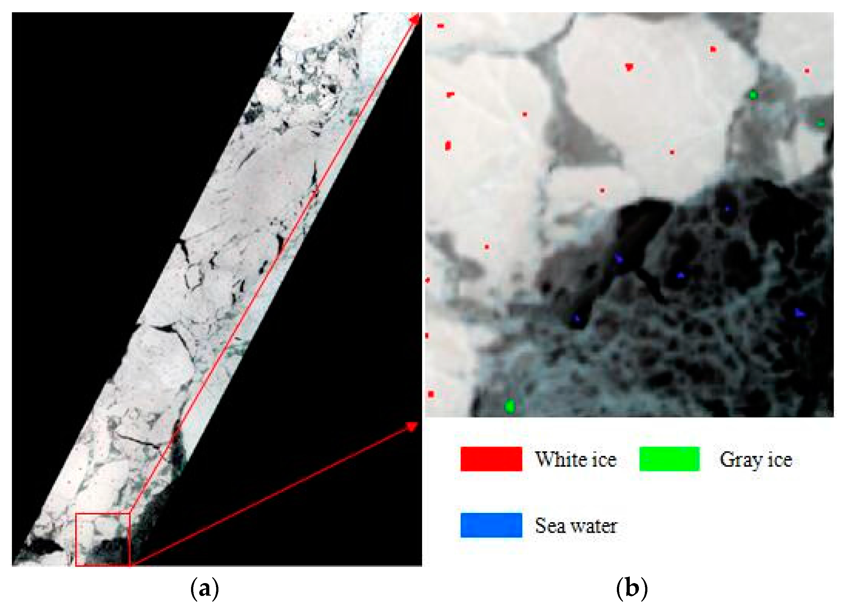
| Class | Training Samples |
|---|---|
| White ice | 2031 |
| Gray ice | 723 |
| Sea water | 549 |
| Total | 3303 |
| Pixel Select Proportions | Bands Selected by ISMLP Method |
|---|---|
| All pixels | 21, 120, 83, 8, 79, 81, 42, 85, 94, 9 |
| 1/20 | 21, 120, 83, 8, 79, 81, 42, 85, 94, 9 |
| 1/40 | 21, 120, 83, 8, 79, 81, 42, 85, 94, 9 |
| 1/60 | 21, 120, 83, 8, 79, 81, 42, 85, 94, 9 |
| 1/80 | 21, 120, 83, 8, 79, 81, 42, 85, 94, 9 |
| 1/100 | 21, 120, 83, 8, 79, 81, 42, 94, 86, 9 |
| 1/1000 | 20, 120, 84, 79, 8, 82, 39, 91, 9, 94 |
© 2017 by the authors. Licensee MDPI, Basel, Switzerland. This article is an open access article distributed under the terms and conditions of the Creative Commons Attribution (CC BY) license (http://creativecommons.org/licenses/by/4.0/).
Share and Cite
Han, Y.; Li, J.; Zhang, Y.; Hong, Z.; Wang, J. Sea Ice Detection Based on an Improved Similarity Measurement Method Using Hyperspectral Data. Sensors 2017, 17, 1124. https://doi.org/10.3390/s17051124
Han Y, Li J, Zhang Y, Hong Z, Wang J. Sea Ice Detection Based on an Improved Similarity Measurement Method Using Hyperspectral Data. Sensors. 2017; 17(5):1124. https://doi.org/10.3390/s17051124
Chicago/Turabian StyleHan, Yanling, Jue Li, Yun Zhang, Zhonghua Hong, and Jing Wang. 2017. "Sea Ice Detection Based on an Improved Similarity Measurement Method Using Hyperspectral Data" Sensors 17, no. 5: 1124. https://doi.org/10.3390/s17051124
APA StyleHan, Y., Li, J., Zhang, Y., Hong, Z., & Wang, J. (2017). Sea Ice Detection Based on an Improved Similarity Measurement Method Using Hyperspectral Data. Sensors, 17(5), 1124. https://doi.org/10.3390/s17051124