
Diagnosis by Volatile Organic Compounds in Exhaled Breath from Lung Cancer Patients Using Support Vector Machine Algorithm


Abstract
:1. Introduction
2. Breath Gas Analysis and Diagnosis Methods
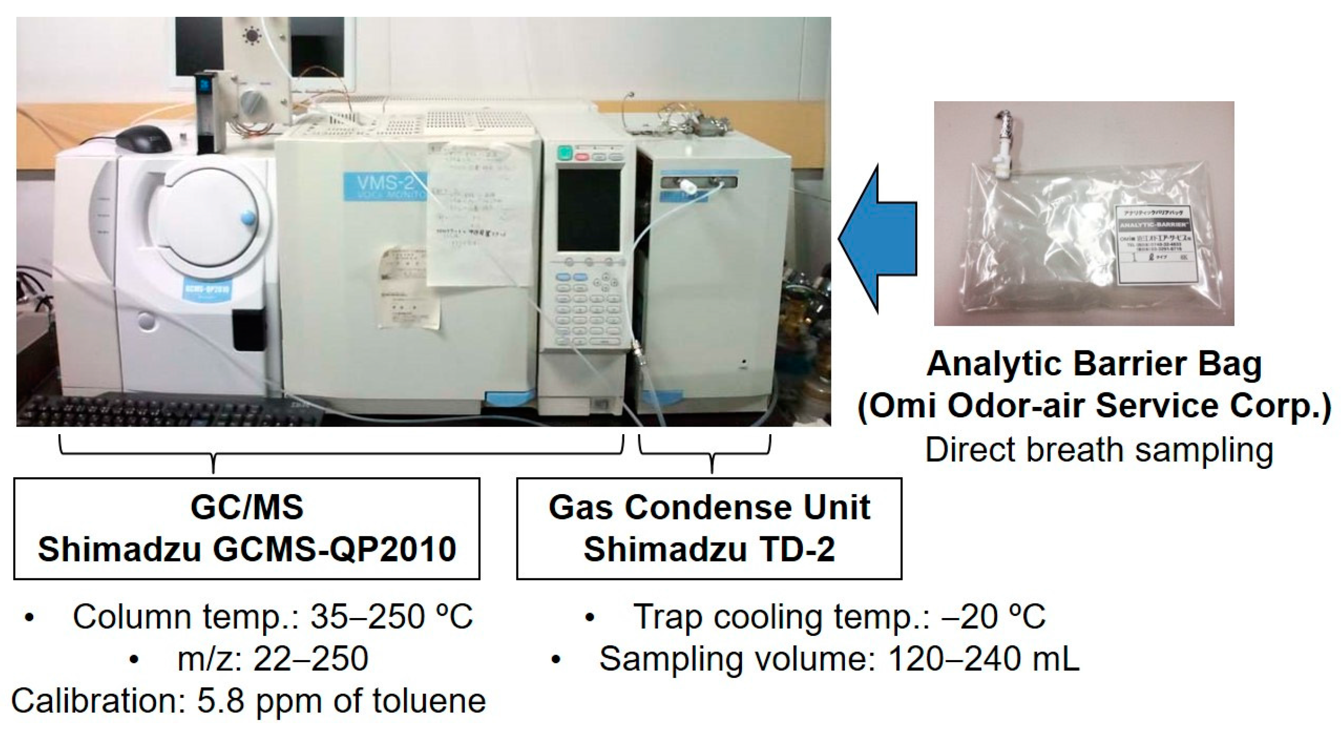
2.1. Breath Collection and Analysis
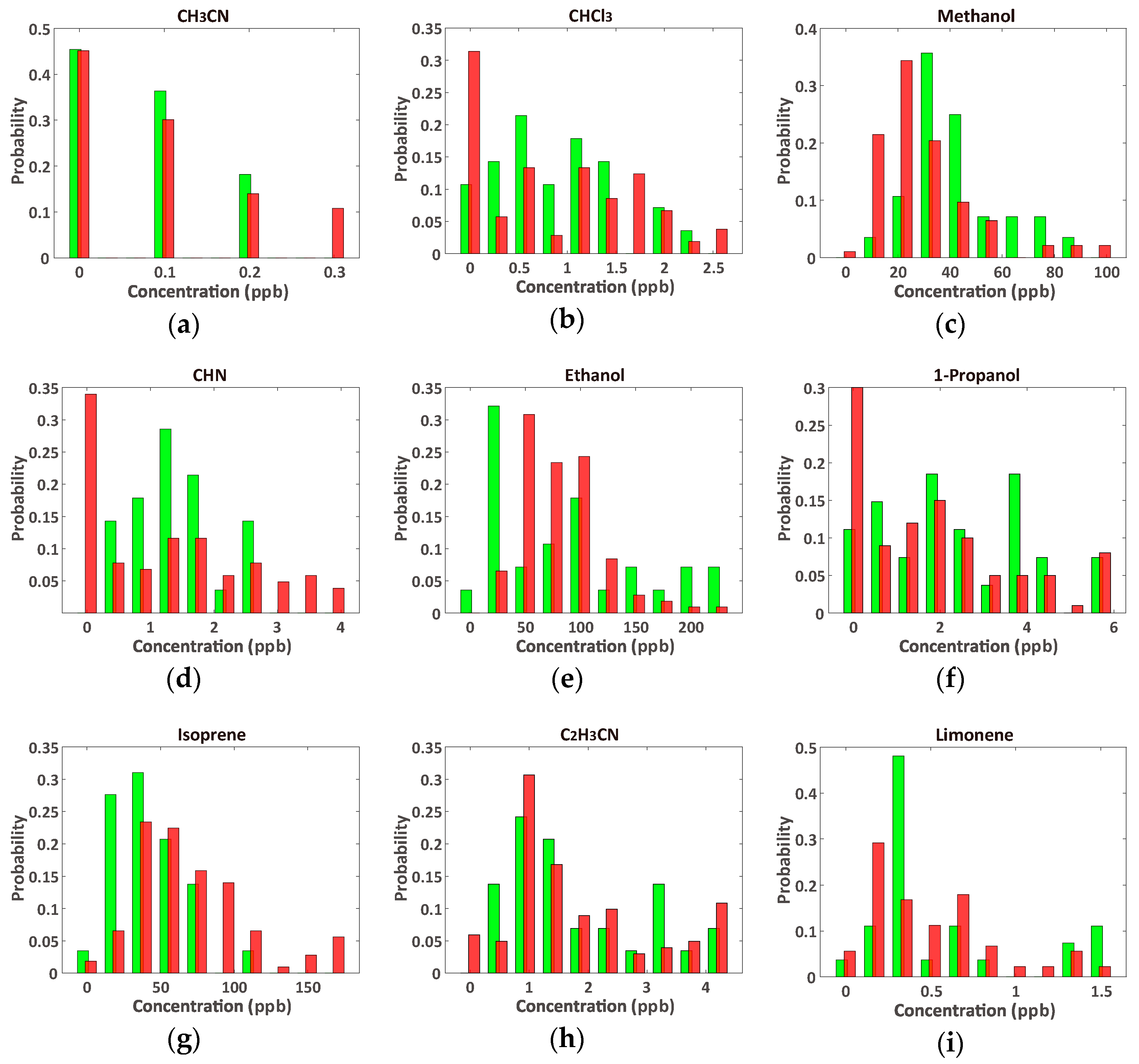
2.2. Data Sets
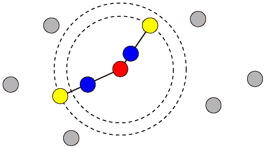
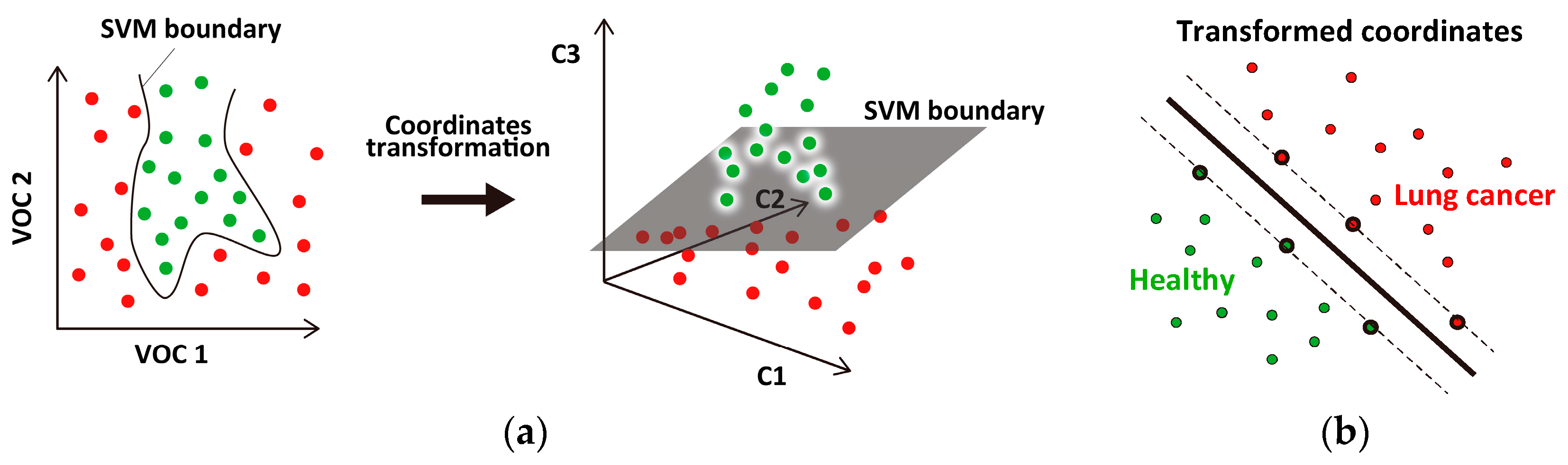
2.3. SVM Classifier
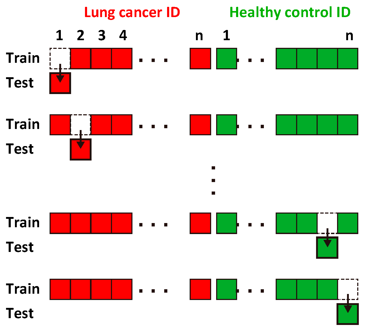
2.4. Evaluation of Classification Accuracy
3. Results and Discussion
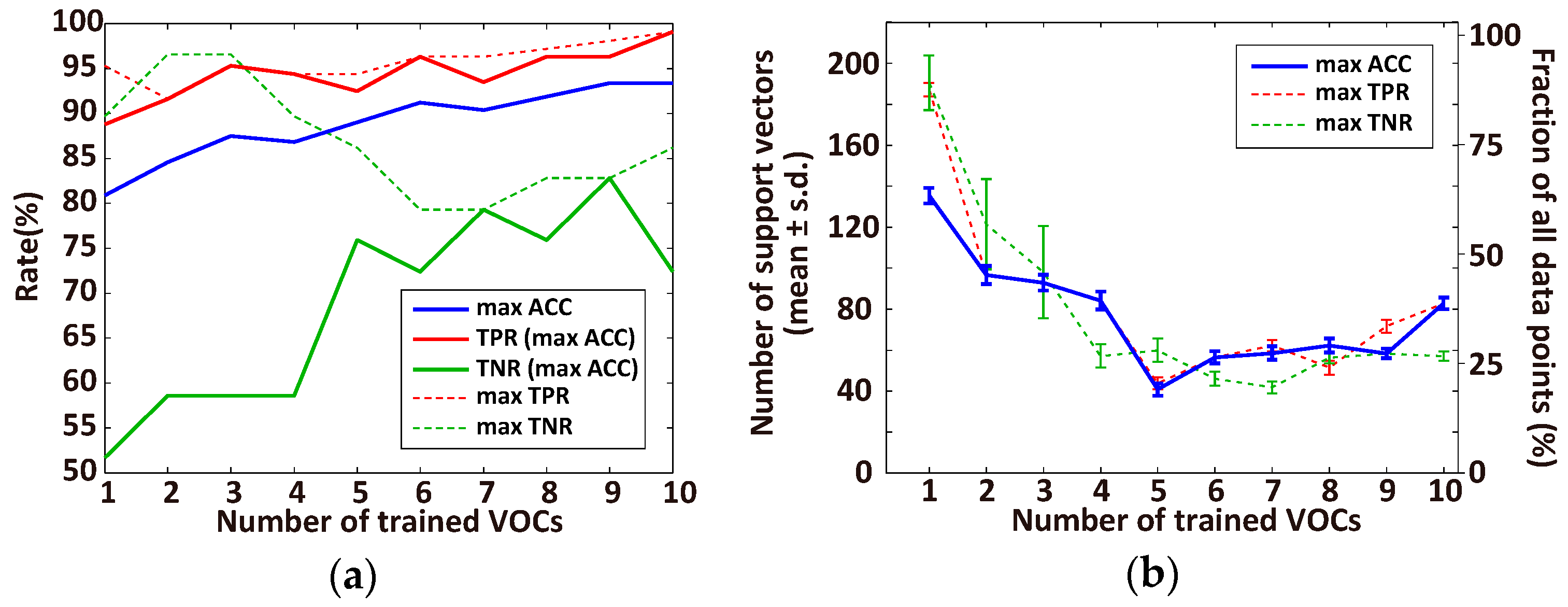
3.1. Optimal Number of VOCs for Classification
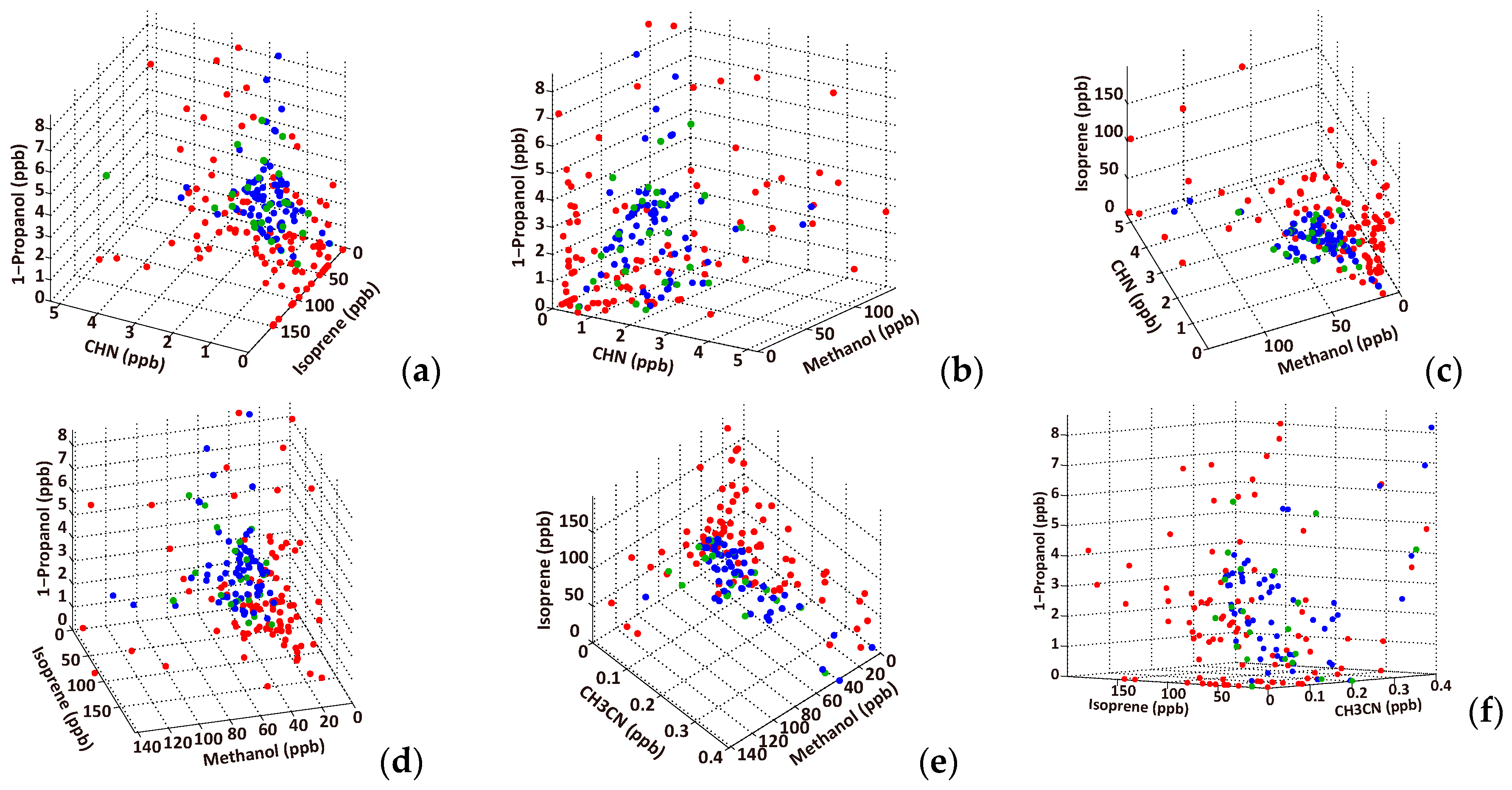
3.2. Effective VOC Combinations for Diagnosing Lung Cancer
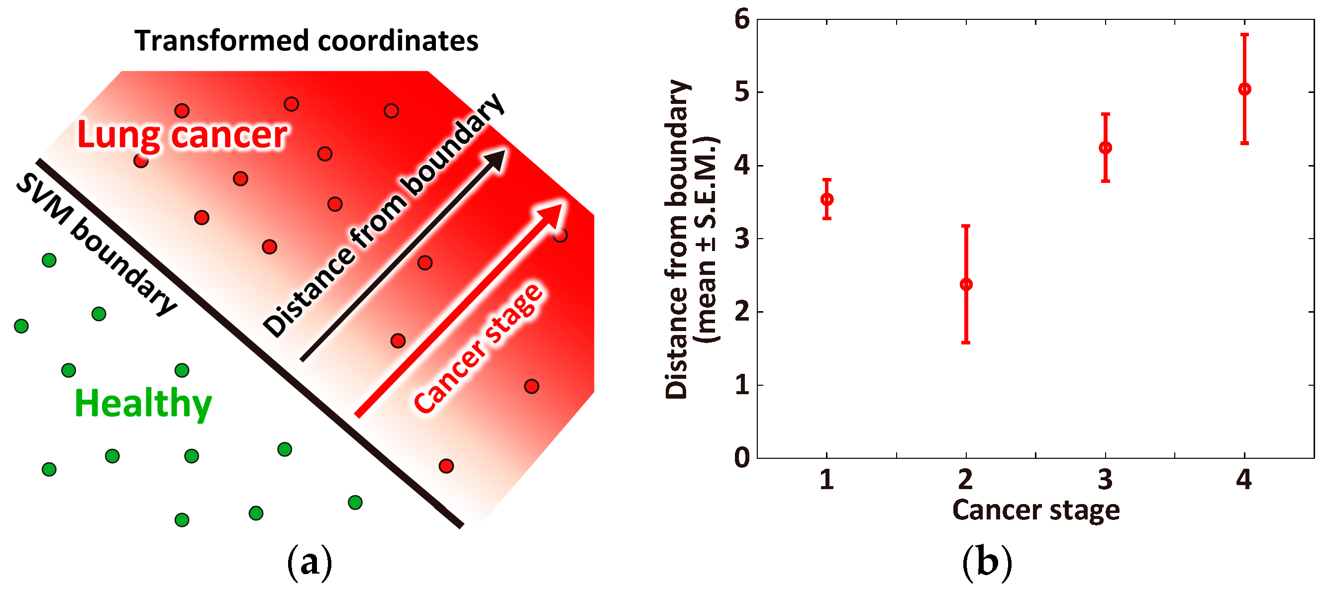
3.3. Correlation between Cancer Stage and Distance from the Classification Boundary
4. Summary and Conclusions
Supplementary Materials
Acknowledgments
Author Contributions
Conflicts of Interest
References
- Gordon, S.; Szidon, J.; Krotoszynski, B.; Gibbons, R.; O’Neill, H. Volatile organic compounds in exhaled air from patients with lung cancer. Clin. Chem. 1985, 31, 1278–1282. [Google Scholar] [PubMed]
- Kharitonov, S.A.; Barnes, P.J. Biomarkers of some pulmonary diseases in exhaled breath. Biomarkers 2002, 7, 1–32. [Google Scholar] [CrossRef] [PubMed]
- Bach, P.B.; Kelley, M.J.; Tate, R.C.; McCrory, D.C. Screening for lung cancer: A review of the current literature. Chest 2003, 123, 72S–82S. [Google Scholar] [CrossRef] [PubMed]
- Corazza, G.; Menozzi, M.; Strocchi, A.; Rasciti, L.; Vaira, D.; Lecchini, R.; Avanzini, P.; Chezzi, C.; Gasbarrini, G. The diagnosis of small bowel bacterial overgrowth. Reliability of jejunal culture and inadequacy of breath hydrogen testing. Gastroenterology 1990, 98, 302–309. [Google Scholar] [CrossRef]
- Phillips, M.; Gleeson, K.; Hughes, J.M.B.; Greenberg, J.; Cataneo, R.N.; Baker, L.; McVay, W.P. Volatile organic compounds in breath as markers of lung cancer: A cross-sectional study. Lancet 1999, 353, 1930–1933. [Google Scholar] [CrossRef]
- Amann, A.; Poupart, G.; Telser, S.; Ledochowski, M.; Schmid, A.; Mechtcheriakov, S. Applications of breath gas analysis in medicine. Int. J. Mass Spectrom. 2004, 239, 227–233. [Google Scholar] [CrossRef]
- Amann, A.; Smith, D. Breath Analysis for Clinical Diagnosis and Therapeutic Monitoring: (With CD-ROM); World Scientific: Singapore, 2005. [Google Scholar]
- Machado, R.F.; Laskowski, D.; Deffenderfer, O.; Burch, T.; Zheng, S.; Mazzone, P.J.; Mekhail, T.; Jennings, C.; Stoller, J.K.; Pyle, J. Detection of lung cancer by sensor array analyses of exhaled breath. Am. J. Respir. Crit. Care Med. 2005, 171, 1286–1291. [Google Scholar] [CrossRef] [PubMed]
- Wehinger, A.; Schmid, A.; Mechtcheriakov, S.; Ledochowski, M.; Grabmer, C.; Gastl, G.A.; Amann, A. Lung cancer detection by proton transfer reaction mass-spectrometric analysis of human breath gas. Int. J. Mass Spectrom. 2007, 265, 49–59. [Google Scholar] [CrossRef]
- Mazzone, P.J. Analysis of volatile organic compounds in the exhaled breath for the diagnosis of lung cancer. J. Thorac. Oncol. 2008, 3, 774–780. [Google Scholar] [CrossRef] [PubMed]
- Fuchs, P.; Loeseken, C.; Schubert, J.K.; Miekisch, W. Breath gas aldehydes as biomarkers of lung cancer. Int. J. Cancer 2010, 126, 2663–2670. [Google Scholar] [CrossRef] [PubMed]
- Lourenco, C.; Turner, C. Breath analysis in disease diagnosis: Methodological considerations and applications. Metabolites 2014, 4, 465–498. [Google Scholar] [CrossRef] [PubMed]
- Phillips, M.; Cataneo, R.N.; Cummin, A.R.; Gagliardi, A.J.; Gleeson, K.; Greenberg, J.; Maxfield, R.A.; Rom, W.N. Detection of lung cancer with volatile markers in the breath. Chest J. 2003, 123, 2115–2123. [Google Scholar] [CrossRef]
- Di Natale, C.; Macagnano, A.; Martinelli, E.; Paolesse, R.; D’Arcangelo, G.; Roscioni, C.; Finazzi-Agrò, A.; D’Amico, A. Lung cancer identification by the analysis of breath by means of an array of non-selective gas sensors. Biosens. Bioelectron. 2003, 18, 1209–1218. [Google Scholar] [CrossRef]
- Phillips, M.; Altorki, N.; Austin, J.H.; Cameron, R.B.; Cataneo, R.N.; Greenberg, J.; Kloss, R.; Maxfield, R.A.; Munawar, M.I.; Pass, H.I. Prediction of lung cancer using volatile biomarkers in breath. Cancer Biomark. 2007, 3, 95–109. [Google Scholar] [CrossRef] [PubMed]
- Peng, G.; Tisch, U.; Adams, O.; Hakim, M.; Shehada, N.; Broza, Y.Y.; Billan, S.; Abdah-Bortnyak, R.; Kuten, A.; Haick, H. Diagnosing lung cancer in exhaled breath using gold nanoparticles. Nat. Nanotechnol. 2009, 4, 669–673. [Google Scholar] [CrossRef] [PubMed]
- Dragonieri, S.; Annema, J.T.; Schot, R.; van der Schee, M.P.; Spanevello, A.; Carratú, P.; Resta, O.; Rabe, K.F.; Sterk, P.J. An electronic nose in the discrimination of patients with non-small cell lung cancer and COPD. Lung Cancer 2009, 64, 166–170. [Google Scholar] [CrossRef] [PubMed]
- Mazzone, P.J.; Wang, X.-F.; Xu, Y.; Mekhail, T.; Beukemann, M.C.; Na, J.; Kemling, J.W.; Suslick, K.S.; Sasidhar, M. Exhaled breath analysis with a colorimetric sensor array for the identification and characterization of lung cancer. J. Thorac. Oncol. 2012, 7, 137–142. [Google Scholar] [CrossRef] [PubMed]
- Pennazza, G.; Santonico, M.; Martinelli, E.; D’Amico, A.; Di Natale, C. Interpretation of exhaled volatile organic compounds. In Exhaled Biomarkers; European Respiratory Society: Lausanne, Switzerland, 2010. [Google Scholar]
- Mazzone, P.J.; Hammel, J.; Dweik, R.; Na, J.; Czich, C.; Laskowski, D.; Mekhail, T. Diagnosis of lung cancer by the analysis of exhaled breath with a colorimetric sensor array. Thorax 2007, 62, 565–568. [Google Scholar] [CrossRef] [PubMed]
- Phillips, M.; Altorki, N.; Austin, J.H.; Cameron, R.B.; Cataneo, R.N.; Kloss, R.; Maxfield, R.A.; Munawar, M.I.; Pass, H.I.; Rashid, A. Detection of lung cancer using weighted digital analysis of breath biomarkers. Clin. Chim. Acta 2008, 393, 76–84. [Google Scholar] [CrossRef] [PubMed]
- Vapnik, V.; Lerner, A. Pattern recognition using generalized portrait method. Autom. Remote Control 1963, 24, 774–780. [Google Scholar]
- Ruan, S.; Lebonvallet, S.; Merabet, A.; Constans, J.-M. Tumor segmentation from a multispectral MRI images by using support vector machine classification. In Proceedings of the 2007 4th IEEE International Symposium on Biomedical Imaging: From Nano to Macro, Arlington, VA, USA, 12–15 April 2007; pp. 1236–1239.
- Zacharaki, E.I.; Wang, S.; Chawla, S.; Soo Yoo, D.; Wolf, R.; Melhem, E.R.; Davatzikos, C. Classification of brain tumor type and grade using MRI texture and shape in a machine learning scheme. Magn. Reson. Med. 2009, 62, 1609–1618. [Google Scholar] [CrossRef] [PubMed]
- Klöppel, S.; Stonnington, C.M.; Chu, C.; Draganski, B.; Scahill, R.I.; Rohrer, J.D.; Fox, N.C.; Jack, C.R.; Ashburner, J.; Frackowiak, R.S. Automatic classification of MR scans in Alzheimer’s disease. Brain 2008, 131, 681–689. [Google Scholar] [CrossRef] [PubMed]
- Ortiz, A.; Górriz, J.M.; Ramírez, J.; Martínez-Murcia, F.J. LVQ-SVM based CAD tool applied to structural MRI for the diagnosis of the Alzheimer’s disease. Pattern Recognit. Lett. 2013, 34, 1725–1733. [Google Scholar] [CrossRef]
- Marquand, A.F.; Mourão-Miranda, J.; Brammer, M.J.; Cleare, A.J.; Fu, C.H. Neuroanatomy of verbal working memory as a diagnostic biomarker for depression. Neuroreport 2008, 19, 1507–1511. [Google Scholar] [CrossRef] [PubMed]
- Nouretdinov, I.; Costafreda, S.G.; Gammerman, A.; Chervonenkis, A.; Vovk, V.; Vapnik, V.; Fu, C.H. Machine learning classification with confidence: Application of transductive conformal predictors to MRI-based diagnostic and prognostic markers in depression. Neuroimage 2011, 56, 809–813. [Google Scholar] [CrossRef] [PubMed]
- Barash, O.; Peled, N.; Tisch, U.; Bunn, P.A., Jr.; Hirsch, F.R.; Haick, H. Classification of lung cancer histology by gold nanoparticle sensors. Nanomedicine 2012, 8, 580–589. [Google Scholar] [CrossRef] [PubMed]
- Van Berkel, J.J.; Dallinga, J.W.; Moller, G.M.; Godschalk, R.W.; Moonen, E.; Wouters, E.F.; van Schooten, F.J. Development of accurate classification method based on the analysis of volatile organic compounds from human exhaled air. J. Chromatogr. B 2008, 861, 101–107. [Google Scholar] [CrossRef] [PubMed]
- Van Berkel, J.J.; Dallinga, J.W.; Moller, G.M.; Godschalk, R.W.; Moonen, E.J.; Wouters, E.F.; van Schooten, F.J. A profile of volatile organic compounds in breath discriminates COPD patients from controls. Respir. Med. 2010, 104, 557–563. [Google Scholar] [CrossRef] [PubMed]
- Hakim, M.; Billan, S.; Tisch, U.; Peng, G.; Dvrokind, I.; Marom, O.; Abdah-Bortnyak, R.; Kuten, A.; Haick, H. Diagnosis of head-and-neck cancer from exhaled breath. Br. J. Cancer 2011, 104, 1649–1655. [Google Scholar] [CrossRef] [PubMed]
- Itoh, T.; Miwa, T.; Tsuruta, A.; Akamatsu, T.; Izu, N.; Shin, W.; Park, J.; Hida, T.; Eda, T.; Setoguchi, Y. Development of an Exhaled Breath Monitoring System with Semiconductive Gas Sensors, a Gas Condenser Unit, and Gas Chromatograph Columns. Sensors 2016, 16, 1891–1906. [Google Scholar] [CrossRef] [PubMed]
- Chawla, N.V.; Bowyer, K.W.; Hall, L.O.; Kegelmeyer, W.P. SMOTE: Synthetic minority over-sampling technique. J. Artif. Intell. Res. 2002, 16, 321–357. [Google Scholar]
- Akbani, R.; Kwek, S.; Japkowicz, N. Applying support vector machines to imbalanced datasets. In Machine Learning: ECML 2004, Proceedings of the 15th European Conference on Machine Learning, Pisa, Italy, 20–24 September 2004; Springer: Berlin/Heidelberg, Germany, 2004; pp. 39–50. [Google Scholar]
- Chawla, N.V. Data mining for imbalanced datasets: An overview. In Data Mining and Knowledge Discovery Handbook; Springer: Berlin/Heidelberg, Germany, 2005; pp. 853–867. [Google Scholar]
- Bernhard, E.B.; Isabelle, M.G.; Vapnik, V.N. A training algorithm for optimal margin classifiers. In Proceedings of the Fifth Annual Workshop on Computational Learning Theory, Pittsburgh, PA, USA, 27–29 July 1992; pp. 144–152.
- Furey, T.S.; Cristianini, N.; Duffy, N.; Bednarski, D.W.; Schummer, M.; Haussler, D. Support vector machine classification and validation of cancer tissue samples using microarray expression data. Bioinformatics 2000, 16, 906–914. [Google Scholar] [CrossRef] [PubMed]
- Brown, M.P.; Grundy, W.N.; Lin, D.; Cristianini, N.; Sugnet, C.W.; Furey, T.S.; Ares, M.; Haussler, D. Knowledge-based analysis of microarray gene expression data by using support vector machines. Proc. Natl. Acad. Sci. USA 2000, 97, 262–267. [Google Scholar] [CrossRef] [PubMed]
- Chai, H.; Domeniconi, C. An evaluation of gene selection methods for multi-class microarray data classification. In Proceedings of the Second European Workshop on Data Mining and Text Mining in Bioinformatics, Pisa, Italy, 20–24 September 2004; pp. 3–10.
- McHardy, A.C.; Martin, H.G.; Tsirigos, A.; Hugenholtz, P.; Rigoutsos, I. Accurate phylogenetic classification of variable-length DNA fragments. Nat. Methods 2007, 4, 63–72. [Google Scholar] [CrossRef] [PubMed]
- Yin, Z.; Sadok, A.; Sailem, H.; McCarthy, A.; Xia, X.; Li, F.; Garcia, M.A.; Evans, L.; Barr, A.R.; Perrimon, N. A screen for morphological complexity identifies regulators of switch-like transitions between discrete cell shapes. Nat. Cell Biol. 2013, 15, 860–871. [Google Scholar] [CrossRef] [PubMed]
- Van’t Veer, L.J.; Dai, H.; van de Vijver, M.J.; He, Y.D.; Hart, A.A.; Mao, M.; Peterse, H.L.; van der Kooy, K.; Marton, M.J.; Witteveen, A.T. Gene expression profiling predicts clinical outcome of breast cancer. Nature 2002, 415, 530–536. [Google Scholar] [CrossRef] [PubMed]
- Ambroise, C.; McLachlan, G.J. Selection bias in gene extraction on the basis of microarray gene-expression data. Proc. Natl. Acad. Sci. USA 2002, 99, 6562–6566. [Google Scholar] [CrossRef] [PubMed]
- Phillips, M.; Cataneo, R.N.; Condos, R.; Erickson, G.A.R.; Greenberg, J.; La Bombardi, V.; Munawar, M.I.; Tietje, O. Volatile biomarkers of pulmonary tuberculosis in the breath. Tuberculosis 2007, 87, 44–52. [Google Scholar] [CrossRef] [PubMed]
- Fens, N.; Zwinderman, A.H.; van der Schee, M.P.; de Nijs, S.B.; Dijkers, E.; Roldaan, A.C.; Cheung, D.; Bel, E.H.; Sterk, P.J. Exhaled breath profiling enables discrimination of chronic obstructive pulmonary disease and asthma. Am. J. Respir. Crit. Care Med. 2009, 180, 1076–1082. [Google Scholar] [CrossRef] [PubMed]
- Gilad-Bachrach, R.; Navot, A.; Tishby, N. Margin based feature selection-theory and algorithms. In Proceedings of the Twenty-First International Conference on Machine Learning, Banff, AB, Canada, 4–8 July 2004; pp. 144–152.
- Navot, A.; Shpigelman, L.; Tishby, N.; Vaadia, E. Nearest neighbor based feature selection for regression and its application to neural activity. Adv. Neural Inf. Process. Syst. 2006, 18, 995–1002. [Google Scholar]
- Klöppel, S.; Abdulkadir, A.; Jack, C.R.; Koutsouleris, N.; Mourão-Miranda, J.; Vemuri, P. Diagnostic neuroimaging across diseases. Neuroimage 2012, 61, 457–463. [Google Scholar] [CrossRef] [PubMed]


| Butane †,‡ | CH3CN †,‡ | CHCl3 †,‡ | Methanol † | Acetone ‡ |
|---|---|---|---|---|
| CHN ‡ | Ethanol ‡ | 1-Propanol | 2-Propanol | C8H16 |
| Isoprene | Dichlorobenzene | C8H17OH | Xylene | Methylcyclohexane |
| Toluene | C2H3CN | Limonene | Nonanal | Unknown 1 |
| Rank | 1 | 2 | 2 | 2 | 2 | 6 | 6 | 6 | 9 | 9 |
|---|---|---|---|---|---|---|---|---|---|---|
| ACC | 89.0 | 88.2 | 88.2 | 88.2 | 88.2 | 86.8 | 86.8 | 86.8 | 86.0 | 86.0 |
| TPR | 92.5 | 91.6 | 93.5 | 91.6 | 92.5 | 91.6 | 89.7 | 92.5 | 91.6 | 87.9 |
| TNR | 75.9 | 75.9 | 69.0 | 75.9 | 72.4 | 69.0 | 75.9 | 65.5 | 65.5 | 79.3 |
| VOCs | CHN | CHN | Methanol | Methanol | Butane | CHN | CHN | C2H3CN | CHN | CHN |
| Methanol | CH3CN | Acetone | Isoprene | CH3CN | Methanol | Butane | Isoprene | Ethanol | CH3CN | |
| CH3CN | C2H3CN | C2H3CN | Xylene | Isoprene | CH3CN | CH3CN | 1-Propanol | Isoprene | Isoprene | |
| Isoprene | Isoprene | Isoprene | Unknown-1 | 1-Propanol | 1-Propanol | Isoprene | Unknown-1 | 1-Propanol | CHCl3 | |
| 1-Propanol | CHCl3 | 1-Propanol | C8H17OH | Xylene | MC | CHCl3 | C8H17OH | Toluene | Xylene |
| Rank | 1 | 2 | 3 | 3 | 3 | 3 | 3 | 3 | 3 | 10 |
|---|---|---|---|---|---|---|---|---|---|---|
| ACC | 84.6 | 88.2 | 86.0 | 89.0 | 84.6 | 88.2 | 85.3 | 85.3 | 86.8 | 86.8 |
| TPR | 94.4 | 93.5 | 92.5 | 92.5 | 92.5 | 92.5 | 92.5 | 92.5 | 92.5 | 91.6 |
| TNR | 48.3 | 69.0 | 62.1 | 75.9 | 55.2 | 72.4 | 58.6 | 58.6 | 65.5 | 69.0 |
| VOCs | Butane | Methanol | Ethanol | CHN | CHN | Butane | Ethanol | Ethanol | C2H3CN | CHN |
| Ethanol | Acetone | CH3CN | Methanol | Ethanol | CH3CN | CH3CN | CH3CN | Isoprene | Methanol | |
| Acetone | C2H3CN | C2H3CN | CH3CN | C2H3CN | Isoprene | Acetone | MC | 1-Propanol | CH3CN | |
| C2H3CN | Isoprene | Isoprene | Isoprene | 1-Propanol | 1-Propanol | 2-Propanol | Unknown-1 | Unknown-1 | 1-Propanol | |
| Toluene | 1-Propanol | 1-Propanol | 1-Propanol | CHCl3 | Xylene | C2H3CN | C8H17OH | C8H17OH | MC |
| Rank | 1 | 2 | 2 | 2 | 5 | 5 | 5 | 5 | 5 | 10 |
|---|---|---|---|---|---|---|---|---|---|---|
| ACC | 84.6 | 89.0 | 88.2 | 84.6 | 88.2 | 85.3 | 86.0 | 85.3 | 86.8 | 86.8 |
| TPR | 82.2 | 86.9 | 76.6 | 78.5 | 77.6 | 79.4 | 72.9 | 78.5 | 71.0 | 83.2 |
| TNR | 89.7 | 86.2 | 86.2 | 86.2 | 82.8 | 82.8 | 82.8 | 82.8 | 82.8 | 79.3 |
| VOCs | CHN | CHN | CHN | CHN | CHN | CHN | Methanol | CH3CN | CH3CN | CHN |
| Isoprene | CH3CN | Methanol | CH3CN | Methanol | Methanol | CH3CN | Acetone | Isoprene | Methanol | |
| Xylene | Isoprene | 2-Propanol | CHCl3 | CH3CN | Isoprene | Isoprene | Unknown-1 | MC | CH3CN | |
| Limonene | CHCl3 | Nonanal | Dichlorobenzene | C2H3CN | Limonene | Limonene | C8H17OH | Nonanal | CHCl3 |
| ACC | TPR | TNR | ||||||
|---|---|---|---|---|---|---|---|---|
| Rank | VOC | Count | Rank | VOC | Count | Rank | VOC | Count |
| 1 | Isoprene | 9 | 1 | 1-Propanol | 7 | 1 | CHN | 7 |
| 2 | CHN | 6 | 2 | C2H3CN | 6 | 1 | CH3CN | 7 |
| 2 | 1-Propanol | 6 | 2 | CH3CN | 6 | 3 | Methanol | 5 |
| 2 | CH3CN | 6 | 4 | Ethanol | 5 | 3 | Isoprene | 5 |
| 5 | Methanol | 4 | 4 | Isoprene | 5 | 5 | CHCl3 | 3 |
© 2017 by the authors. Licensee MDPI, Basel, Switzerland. This article is an open access article distributed under the terms and conditions of the Creative Commons Attribution (CC BY) license ( http://creativecommons.org/licenses/by/4.0/).
Share and Cite
Sakumura, Y.; Koyama, Y.; Tokutake, H.; Hida, T.; Sato, K.; Itoh, T.; Akamatsu, T.; Shin, W. Diagnosis by Volatile Organic Compounds in Exhaled Breath from Lung Cancer Patients Using Support Vector Machine Algorithm. Sensors 2017, 17, 287. https://doi.org/10.3390/s17020287
Sakumura Y, Koyama Y, Tokutake H, Hida T, Sato K, Itoh T, Akamatsu T, Shin W. Diagnosis by Volatile Organic Compounds in Exhaled Breath from Lung Cancer Patients Using Support Vector Machine Algorithm. Sensors. 2017; 17(2):287. https://doi.org/10.3390/s17020287
Chicago/Turabian StyleSakumura, Yuichi, Yutaro Koyama, Hiroaki Tokutake, Toyoaki Hida, Kazuo Sato, Toshio Itoh, Takafumi Akamatsu, and Woosuck Shin. 2017. "Diagnosis by Volatile Organic Compounds in Exhaled Breath from Lung Cancer Patients Using Support Vector Machine Algorithm" Sensors 17, no. 2: 287. https://doi.org/10.3390/s17020287
APA StyleSakumura, Y., Koyama, Y., Tokutake, H., Hida, T., Sato, K., Itoh, T., Akamatsu, T., & Shin, W. (2017). Diagnosis by Volatile Organic Compounds in Exhaled Breath from Lung Cancer Patients Using Support Vector Machine Algorithm. Sensors, 17(2), 287. https://doi.org/10.3390/s17020287