
A Novel Medical E-Nose Signal Analysis System

Abstract
:1. Introduction
2. Optimal System Design
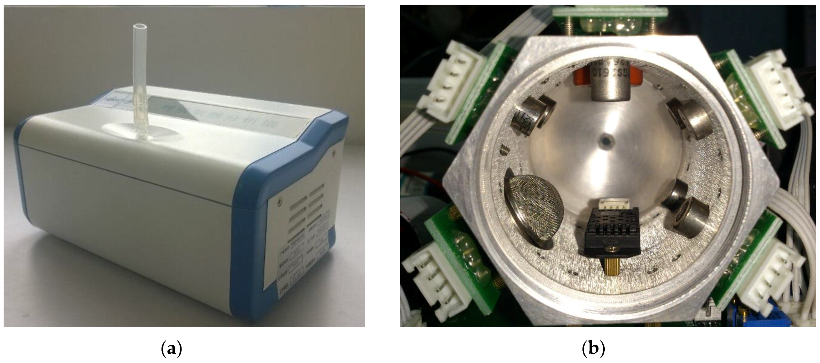
2.1. Sensor Array Selection
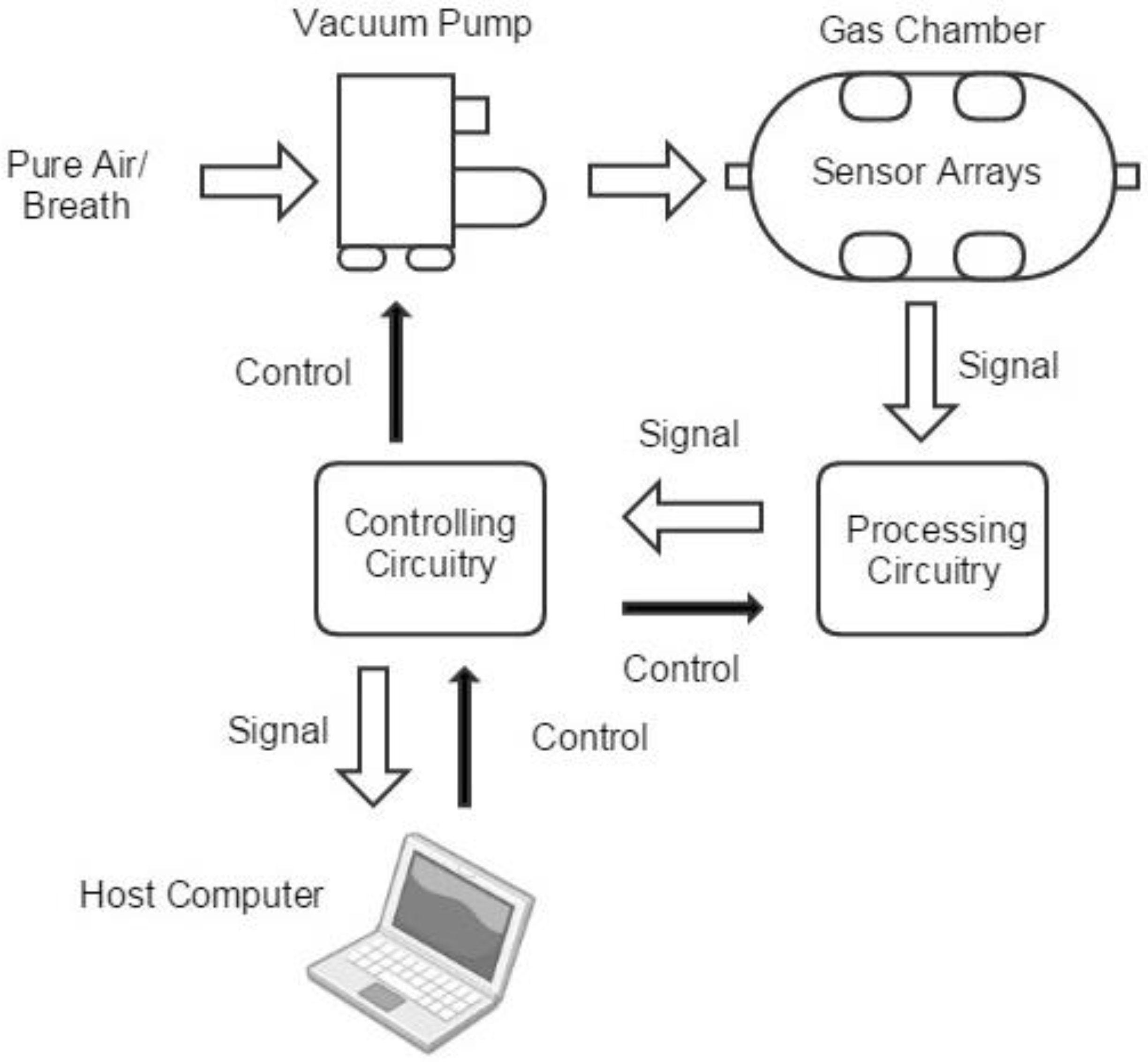
2.2. Optimized System Structure
2.3. Sampling Procedure
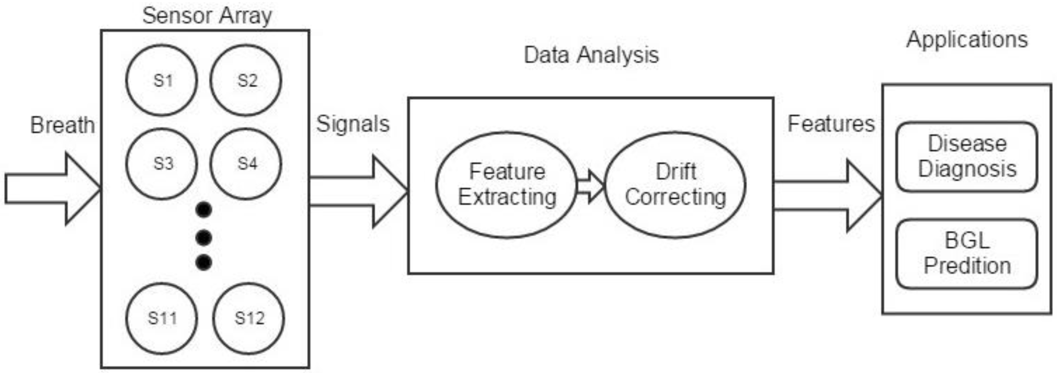
3. Signal Analysis
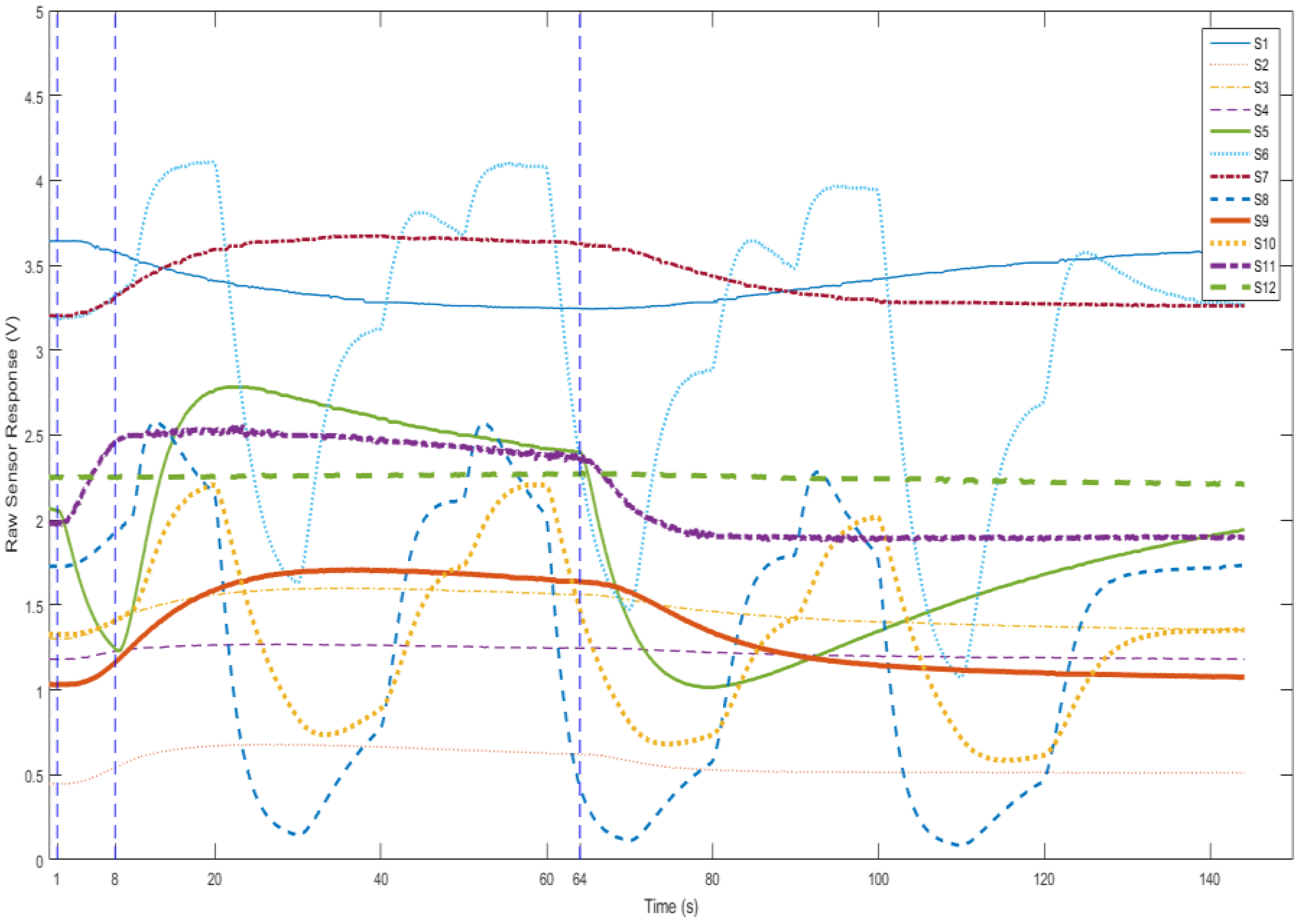
3.1. Preprocessing
3.2. Feature Extraction
3.3. Drift Compensation
3.3.1. Sensor Drift
3.3.2. Optimized MIDA
4. Experiments
4.1. Breath Dataset
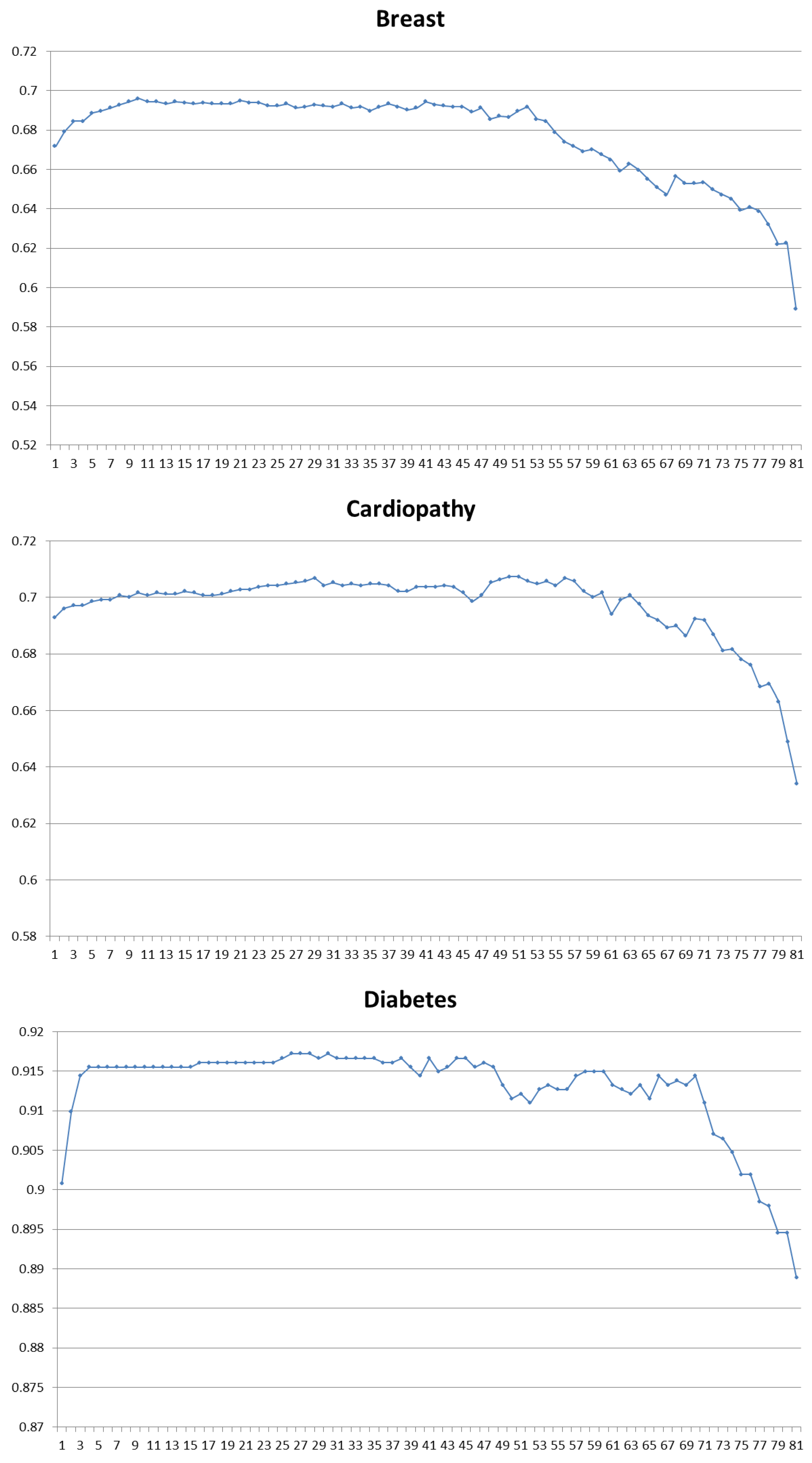
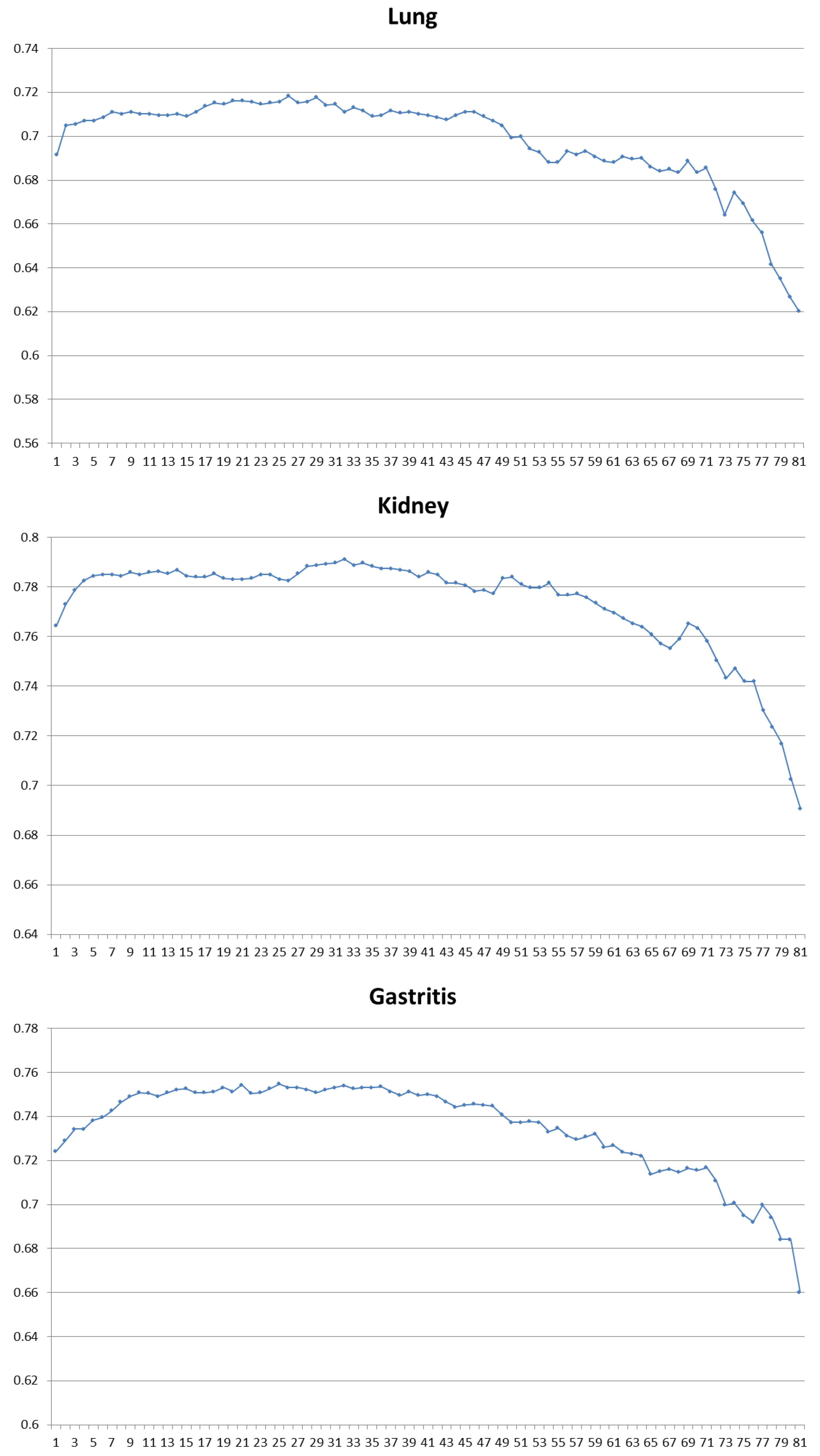
4.2. Disease Diagnosis
4.3. BGL Classification
5. Conclusions
Acknowledgments
Author Contributions
Conflicts of Interest
References
- Röck, F.; Barsan, N.; Weimar, U. Electronic nose: current status and future trends. Chem. Rev. 2008, 108, 705–725. [Google Scholar] [CrossRef] [PubMed]
- Chou, J. Hazardous Gas Monitors: A Practical Guide to Selection, Operation and Applications; McGraw-Hill: New York, NY, USA, 2000. [Google Scholar]
- Zampolli, S.; Elmi, I.; Ahmed, F.; Passini, M.; Cardinali, G.; Nicoletti, S.; Dori, L. An electronic nose based on solid state sensor arrays for low-cost indoor air quality monitoring applications. Sens. Actuators B Chem. 2004, 101, 39–46. [Google Scholar] [CrossRef]
- Romain, A.; Nicolas, J. Long term stability of metal oxide-based gas sensors for e-nose environmental applications: An overview. Sens. Actuators B Chem. 2010, 146, 502–506. [Google Scholar] [CrossRef]
- Zhang, L.; Tian, F.; Nie, H.; Dang, L.; Li, G.; Ye, Q.; Kadri, C. Classification of multiple indoor air contaminants by an electronic nose and a hybrid support vector machine. Sens. Actuators B Chem. 2012, 174, 114–125. [Google Scholar] [CrossRef]
- Aeonose and Aeolus Bring Tail Wind. Available online: http://www.enose.nl/products/aeonose/ (access on 30 January 2017).
- Portable Electronic Nose | AIRSENSE Analytics. Available online: http://www.airsense.com/en/products/portable-electronic-nose/ (accessed on 30 January 2017).
- HERACLES Electronic Nose, Instrument for Sensory Analysis. Available online: http://www.alpha-mos.com/analytical-instruments/heracles-electronic-nose.php (accessed on 30 January 2017).
- Cyranose Electronic Nose. Available online: http://www.sensigent.com/products/cyranose.html (accessed on 30 January 2017).
- COMPUTER INTEGRATED zNose® Model 4600. Available online: http://www.estcal.com/product/computer-integrated-znoser (accessed on 30 January 2017).
- Lonestar Gas Analyzer. Available online: http://www.owlstonenanotech.com/lonestar (accessed on 30 January 2017).
- Lin, Y.; Guo, H.; Chang, Y.; Kao, M.; Wang, H.; Hong, R. Application of the electronic nose for uremia diagnosis. Sens. Actuators B Chem. 2001, 76, 177–180. [Google Scholar] [CrossRef]
- Li, J.; Zhang, D.; Li, Y.; Wu, J.; Zhang, B. Joint similar and specific learning for diabetes mellitus and impaired glucose regulation detection. Inf. Sci. 2017, 384, 191–204. [Google Scholar] [CrossRef]
- Yu, J.; Byun, H.; So, M.; Huh, J. Analysis of diabetic patient’s breath with conducting polymer sensor array. Sens. Actuators B Chem. 2005, 108, 305–308. [Google Scholar] [CrossRef]
- Blatt, R.; Bonarini, A.; Calabro, E.; Della Torre, M.; Matteucci, M.; Pastorino, U. In Lung cancer identification by an electronic nose based on an array of MOS sensors. In Proceedings of the 2007 International Joint Conference on Neural Networks, Orlando, FL, USA, 12 August 2007; pp. 1423–1428.
- van Hooren, M.R.; Leunis, N.; Brandsma, D.S.; Dingemans, A.M.C.; Kremer, B.; Kross, K.W. Differentiating head and neck carcinoma from lung carcinoma with an electronic nose: A proof of concept study. Eur. Arch. Oto-Rhino-Laryngol. 2016, 273, 3897–3903. [Google Scholar] [CrossRef] [PubMed]
- Brekelmans, M.P.; Fens, N.; Brinkman, P.; Bos, L.D.; Sterk, P.J.; Tak, P.P.; Gerlag, D.M. Smelling the Diagnosis: The Electronic Nose as Diagnostic Tool in Inflammatory Arthritis. A Case-Reference Study. PloS ONE 2016, 11, e0151715. [Google Scholar]
- Dragonieri, S.; Schot, R.; Mertens, B.J.; Le Cessie, S.; Gauw, S.A.; Spanevello, A.; Resta, O.; Willard, N.P.; Vink, T.J.; Rabe, K.F. An electronic nose in the discrimination of patients with asthma and controls. J. Allergy Clin. Immunol. 2007, 120, 856–862. [Google Scholar] [CrossRef] [PubMed]
- Nakhleh, M.K.; Amal, H.; Jeries, R.; Broza, Y.Y.; Aboud, M.; Gharra, A.; Ivgi, H.; Khatib, S.; Badarneh, S.; Har-Shai, L.; et al. Diagnosis and Classification of 17 Diseases from 1404 Subjects via Pattern Analysis of Exhaled Molecules. ACS Nano 2017, 11, 112–125. [Google Scholar] [CrossRef] [PubMed]
- Phillips, M. Method for the collection and assay of volatile organic compounds in breath. Anal. Biochem. 1997, 247, 272–278. [Google Scholar] [CrossRef] [PubMed]
- Yan, K.; Zhang, D.; Wu, D.; Wei, H.; Lu, G. Design of a breath analysis system for diabetes screening and blood glucose level prediction. IEEE Trans. Biomed. Eng. 2014, 61, 2787–2795. [Google Scholar] [CrossRef] [PubMed]
- Di Natale, C.; Paolesse, R.; Martinelli, E.; Capuano, R. Solid-state gas sensors for breath analysis: A review. Anal. Chim. Acta 2014, 824, 1–17. [Google Scholar] [CrossRef] [PubMed]
- Broza, Y.Y.; Zuri, L.; Haick, H. Combined volatolomics for monitoring of human body chemistry. Sci. Rep. 2014, 4, 4611. [Google Scholar] [CrossRef] [PubMed]
- Risby, T.H.; Solga, S. Current status of clinical breath analysis. Appl. Phys. B 2006, 85, 421–426. [Google Scholar] [CrossRef]
- Ueta, I.; Saito, Y.; Hosoe, M.; Okamoto, M.; Ohkita, H.; Shirai, S.; Tamura, H.; Jinno, K. Breath acetone analysis with miniaturized sample preparation device: In-needle preconcentration and subsequent determination by gas chromatography–mass spectroscopy. J. Chromatogr. B 2009, 877, 2551–2556. [Google Scholar] [CrossRef] [PubMed]
- Wang, C.; Mbi, A.; Shepherd, M. A study on breath acetone in diabetic patients using a cavity ringdown breath analyzer: exploring correlations of breath acetone with blood glucose and glycohemoglobin A1C. IEEE Sens. J. 2010, 10, 54–63. [Google Scholar] [CrossRef]
- Righettoni, M.; Schmid, A.; Amann, A.; Pratsinis, S. Correlations between blood glucose and breath components from portable gas sensors and PTR-TOF-MS. J. Breath Res. 2013, 7, 037110. [Google Scholar] [CrossRef] [PubMed]
- Ghimenti, S.; Tabucchi, S.; Lomonaco, T.; Di Francesco, F.; Fuoco, R.; Onor, M.; Lenzi, S.; Trivella, M. Monitoring breath during oral glucose tolerance tests. J. Breath Res. 2013, 7, 017115. [Google Scholar] [CrossRef] [PubMed]
- Cao, W.; Duan, Y. Current status of methods and techniques for breath analysis. Crit. Rev. Anal. Chem. 2007, 37, 3–13. [Google Scholar] [CrossRef]
- Deykin, A.; Massaro, A.F.; Drazen, J.M.; Israel, E. Exhaled nitric oxide as a diagnostic test for asthma: online versus offline techniques and effect of flow rate. Am. J. Respir. Crit. Care Med. 2002, 165, 1597–1601. [Google Scholar] [CrossRef] [PubMed]
- Davies, S.; Spanel, P.; Smith, D. Quantitative analysis of ammonia on the breath of patients in end-stage renal failure. Kidney Int. 1997, 52, 223–228. [Google Scholar] [CrossRef] [PubMed]
- Phillips, M.; Altorki, N.; Austin, J.H.; Cameron, R.B.; Cataneo, R.N.; Greenberg, J.; Kloss, R.; Maxfield, R.A.; Munawar, M.I.; Pass, H.I. Prediction of lung cancer using volatile biomarkers in breath. Cancer Biomark. 2007, 3, 95–109. [Google Scholar] [CrossRef] [PubMed]
- Phillips, M.; Boehmer, J.P.; Cataneo, R.N.; Cheema, T.; Eisen, H.J.; Fallon, J.T.; Fisher, P.E.; Gass, A.; Greenberg, J.; Kobashigawa, J. Heart allograft rejection: detection with breath alkanes in low levels (the HARDBALL study). J. Heart Lung Transpl. 2004, 23, 701–708. [Google Scholar] [CrossRef]
- Phillips, M.; Cataneo, R.N.; Ditkoff, B.A.; Fisher, P.; Greenberg, J.; Gunawardena, R.; Kwon, C.S.; Rahbari-Oskoui, F.; Wong, C. Volatile markers of breast cancer in the breath. Breast J. 2003, 9, 184–191. [Google Scholar] [CrossRef] [PubMed]
- Eisenmann, A.; Amann, A.; Said, M.; Datta, B.; Ledochowski, M. Implementation and interpretation of hydrogen breath tests. J. Breath Res. 2008, 2, 046002. [Google Scholar] [CrossRef] [PubMed]
- Turner, C. Potential of breath and skin analysis for monitoring blood glucose concentration in diabetes. Exp. Rev. Mol. Diagn. 2011, 11, 497–503. [Google Scholar] [CrossRef] [PubMed]
- Marco, S.; Gutierrez-Galvez, A. Signal and data processing for machine olfaction and chemical sensing: A review. IEEE Sens. J. 2012, 12, 3189–3214. [Google Scholar] [CrossRef]
- Martinelli, E.; Falconi, C.; D’Amico, A.; Di Natale, C. Feature extraction of chemical sensors in phase space. Sens. Actuators B Chem. 2003, 95, 132–139. [Google Scholar] [CrossRef]
- Hierlemann, A.; Gutierrez-Osuna, R. Higher-order chemical sensing. Chem. Rev. 2008, 108, 563–613. [Google Scholar] [CrossRef] [PubMed]
- Phillips, M.; Cataneo, R.N.; Greenberg, J.; Gunawardena, R.; Naidu, A.; Rahbari-Oskoui, F. Effect of age on the breath methylated alkane contour, a display of apparent new markers of oxidative stress. J. Lab. Clin. Med. 2000, 136, 243–249. [Google Scholar] [CrossRef] [PubMed]
- Klaassen, E.M.; van de Kant, K.D.; Jöbsis, Q.; van Schayck, O.C.; Smolinska, A.; Dallinga, J.W.; van Schooten, F.J.; den Hartog, G.J.; de Jongste, J.C.; Rijkers, G.T. Exhaled biomarkers and gene expression at preschool age improve asthma prediction at 6 years of age. Am. J. Respir. Crit. Care Med. 2015, 91, 201–207. [Google Scholar] [CrossRef] [PubMed]
- Zhang, L.; Tian, F.; Kadri, C.; Xiao, B.; Li, H.; Pan, L.; Zhou, H. On-line sensor calibration transfer among electronic nose instruments for monitoring volatile organic chemicals in indoor air quality. Sens. Actuators B Chem. 2011, 160, 899–909. [Google Scholar] [CrossRef]
- Feudale, R.N.; Woody, N.A.; Tan, H.; Myles, A.J.; Brown, S.D.; Ferré, J. Transfer of multivariate calibration models: a review. Chemom. Intell. Lab. Syst. 2002, 64, 181–192. [Google Scholar] [CrossRef]
- Artursson, T.; Eklov, T.; Lundström, I.; Martensson, P.; Sjostrom, M.; Holmberg, M. Drift correction for gas sensors using multivariate methods. J. Chemom. 2000, 14, 711–723. [Google Scholar] [CrossRef]
- Yan, K.; Zhang, D. Correcting Instrumental Variation and Time-Varying Drift: A Transfer Learning Approach with Autoencoders. IEEE Trans. Instrum. Meas. 2016, 65, 2012–2022. [Google Scholar] [CrossRef]
- Gretton, A.; Bousquet, O.; Smola, A.; Schölkopf, B. Measuring statistical dependence with Hilbert-Schmidt norms. In Algorithmic Learning Theory; Springer: New York, NY, USA, 2005; pp. 63–77. [Google Scholar]
- Shang, D. New Concept of Practical Diabetes Prevention; Anhui Science & Technology Publishing House: Hefei, China, 2004. [Google Scholar]


| Manufacturer | Product | Application |
|---|---|---|
| The eNose Company, Rotterdam, The Netherlands | AEONOSE [6] | Medical |
| Airsense Analytics GmnH, Schwerin, Germany | PEN3 [7] | Food, wine, matierial, enviroment, medical |
| Alpha-Mos, Toulouse, France | HERACLES [8] | Food, material, process management |
| Sensigent, Baldwin Park, CA, USA | Cyranose 320 [9] | medical, materials identification, food |
| Electronic Sensor Technology Inc., Newbury Park, CA, USA | Z-Nose [10] | Investigation, food, enviroment, medical |
| Owlstone Inc., Cambridge, UK | LONESTAR [11] | Food, materials, industry |
| Diseases | Breath Biomarkers |
|---|---|
| diabetes [24] | acetone |
| renal disease [31] | ammonia |
| heart disease [33] | propane |
| lung cancer [32] | benzene,1,1-oxybis-, 1,1-biphenyl,2, 2-diethyl, furan,2,5-dimethyl-, etc. |
| breast cancer [34] | nonane, tridecane, 5-methyl, undecane, 3-methyl, etc. |
| digestive system disease [35] | hydrogen |
| Channel | Model | Manufacturer | Function | Sensitivities (ppm) |
|---|---|---|---|---|
| 1 | TGS4161 | Figaro Inc., Osaka, Japan | CO2 | 350–10,000 |
| 2 | TGS826 | Figaro Inc., Osaka, Japan | VOCs, NH3 | 30–5000 |
| 3 | QS01 | FIS Inc., Hyogo, Japan | VOCs, H2, CO | 1–1000 |
| 4 | TGS2610D | Figaro Inc., Osaka, Japan | H2, VOCs | 500–10,000 |
| 5 | TGS822 | Figaro Inc., Osaka, Japan | VOCs, H2, CO | 50–5000 |
| 6 | TGS2602-TM | Figaro Inc., Osaka, Japan | VOCs, NH3, H2S | 1–30 |
| 7 | TGS2602 | Figaro Inc., Osaka, Japan | VOCs, NH3, H2S | 1–30 |
| 8 | TGS2600-TM | Figaro Inc., Osaka, Japan | H2, VOCs, CO | 1–100 |
| 9 | TGS2603 | Figaro Inc., Osaka, Japan | NH3, H2S | 1–10 |
| 10 | TGS2620-TM | Figaro Inc., Osaka, Japan | VOCs, H2 | 50–5000 |
| 11 | HTG3515CH | Humirel Inc., Toulouse, France | Temperature | |
| 12 | Humidity |
| Parameters | Specifications |
|---|---|
| Device size | 22 × 15 × 11 cm |
| Working temperature | 25 ± 10 °C |
| Gas chamber volume | 600 mL |
| Injection rate | 50 mL/s |
| Sampling frequency | 8 Hz |
| Sampling time | 144 s |
| Working voltage | 5 V |
| Working voltage for temperature modulated sensors | 3–7 V cycle |
| Resolution of the Analog-to-Digital Converter (ADC) | 12 bit |
| Feature | Characteristics | |
|---|---|---|
| Spacial | PCA | Reduced dimension of the origin features with PCA method. |
| Magnitude | Down-sampled values of the curve’s magnitude M. The maximum magnitude. Down-sampled values of the normalized magnitude M/max (M). Mean values of the magnitude. | |
| Derivative | Down-sampled values of the curve’s derivative D. The maximum and minimum derivative. | |
| Second derivative | The maximum and minimum second derivative in both the injection and purge stage. | |
| Integral | The integral of the five intervals of the curve; the intervals are the same with the difference feature. | |
| Slope | The slope of the five intervals of the curve; the intervals are the same with the difference feature. | |
| Phase Feature | The phase feature is proposed in [39]. First, the response is transformed to the phase space, which is spanned by its magnitude and derivative. Then, the phase features are defined as | |
| Frequency | FFT | Fast Fourier tranformation |
| Wavelet | Wavelet transformation | |
| Class | Number |
|---|---|
| Healthy | 1291 |
| Diabetes | 491 |
| Kidney disease | 398 |
| Cardiopathy | 537 |
| Lung disease | 376 |
| Breast disease | 527 |
| Gastritis | 241 |
| Task | Features and Sensors | SEN | SPE | ACC | |
|---|---|---|---|---|---|
| Diabetes | Wavelet of TGS2602 Phase of TGS2602-TM | Wavelet of TGS2610D MaxMag of TGS826 | 0.8815 | 0.9495 | 0.9155 |
| Kidney Disease | Wavelet of TGS2602 Slope of TGS2602-TM Phase of TGS826 | Wavelet of TGS2600-TM Slope of TGS2620-TM Phase of TGS2610D | 0.7002 | 0.8698 | 0.7850 |
| Cardiopathy | Wavelet of TGS822 MeanMag of TGS2603 Integral of TGS2602 MaxMag of TGS2603 Phase of TGS2610D | Integral of TGS826 Slope of TGS822 Slope of TGS826 Phase of TGS826 Integral of TGS2610D | 0.7433 | 0.7125 | 0.7279 |
| Lung Disease | Wavelet of QS01 Slope of TGS2603 Integral of TGS2602 Phase of TGS2620-TM MaxMag of TGS2602 MeanMag of TGS2610D MaxMag of TGS2603 Integral of QS01 MaxMag of TGS2602-TM Phase of TGS826 Phase of TGS2602 | MeanMag of QS01 Slope of QS01 Integral of TGS826 Slope of TGS826 Integral of TGS2610D MeanMag of TGS2603 MeanMag of TGS2602-TM MeanMag of TGS2602 MaxMag of TGS826 Phase of QS01 | 0.7117 | 0.7209 | 0.7163 |
| Breast Disease | Wavelet of TGS826 MaxMag of TGS2602 Derivative of TGS2620-TM Phase of TGS2600-TM MeanMag of TGS2602-TM | MaxMag of TGS822 Derivative of TGS2610D MaxMag of TGS2603 MeanMag of TGS2600-TM Phase of TGS2620-TM | 0.6321 | 0.7599 | 0.6960 |
| Gastritis | Wavelet of TGS822 Integral of TGS2603 Phase of TGS2602-TM Wavelet of TGS2620-TM MaxMag of TGS2602-TM | Slope of TGS2600-TM MaxMag of TGS2620-TM Integral of QS01 Derivative of TGS2610D Slope of TGS2603 | 0.6436 | 0.8582 | 0.7509 |
| Class | BGL (mmol/L) | Number |
|---|---|---|
| Normal | Lower than 6.1 | 1851 |
| Impaired glucose tolerance | 6.1–7.11 | 168 |
| Hyperglycemia | Higher than 7.11 | 241 |
| Features and Sensors | Accuracy | |
|---|---|---|
| MaxMag of TGS2602-TM | MaxMag of TGS2602 | 0.7778 |
| MeanMag of TGS2602-TM | DownSample of TGS826 | |
| DownSample of QS01 DownSample of TGS822 Slope of QS01 | DownSample of TGS2610D Slope of TGS826 Integral of QS01 | |
© 2017 by the authors. Licensee MDPI, Basel, Switzerland. This article is an open access article distributed under the terms and conditions of the Creative Commons Attribution (CC BY) license ( http://creativecommons.org/licenses/by/4.0/).
Share and Cite
Kou, L.; Zhang, D.; Liu, D. A Novel Medical E-Nose Signal Analysis System. Sensors 2017, 17, 402. https://doi.org/10.3390/s17040402
Kou L, Zhang D, Liu D. A Novel Medical E-Nose Signal Analysis System. Sensors. 2017; 17(4):402. https://doi.org/10.3390/s17040402
Chicago/Turabian StyleKou, Lu, David Zhang, and Dongxu Liu. 2017. "A Novel Medical E-Nose Signal Analysis System" Sensors 17, no. 4: 402. https://doi.org/10.3390/s17040402
APA StyleKou, L., Zhang, D., & Liu, D. (2017). A Novel Medical E-Nose Signal Analysis System. Sensors, 17(4), 402. https://doi.org/10.3390/s17040402