Textile Pressure Mapping Sensor for Emotional Touch Detection in Human-Robot Interaction

 ,
,  , ,
, , 
Abstract
:1. Introduction
1.1. Contribution
1.2. Paper Structure
2. Sensor Hardware
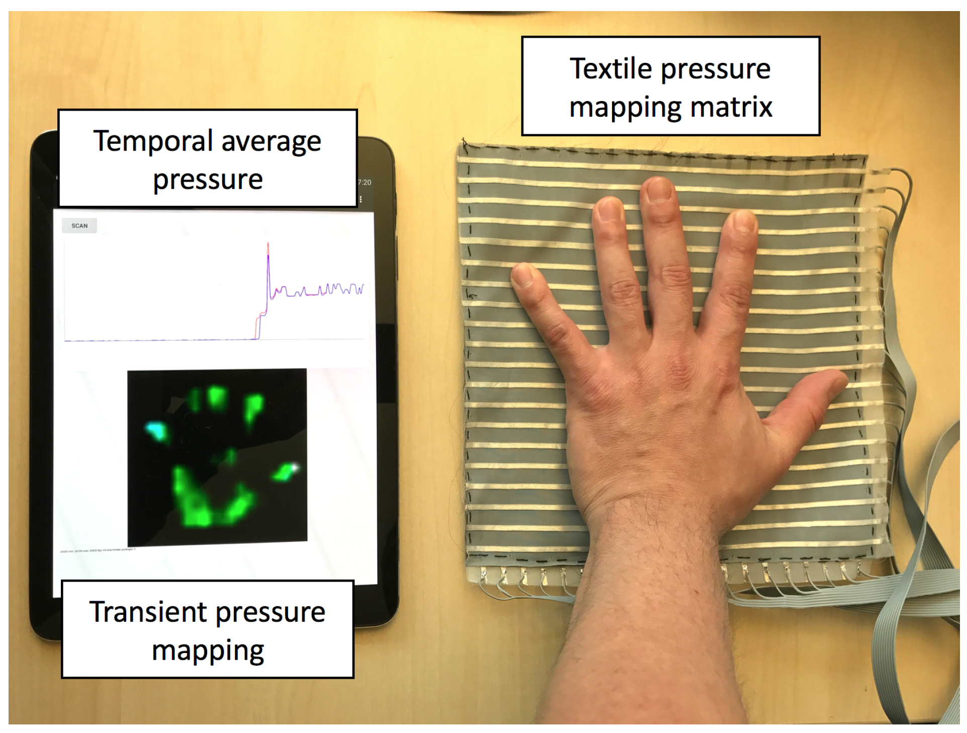
2.1. Sensing Fabrics
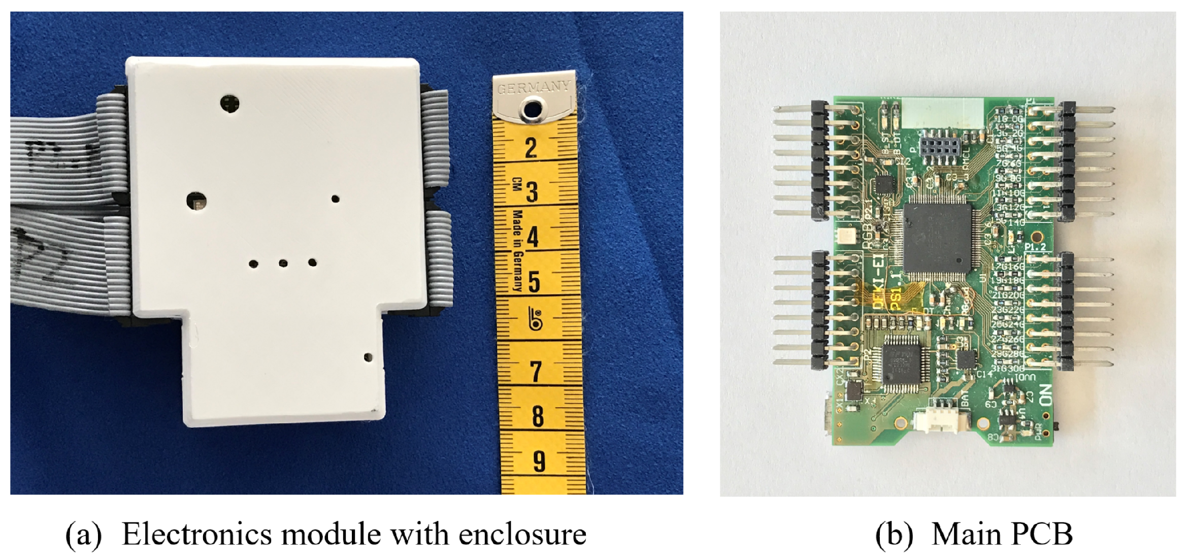
2.2. Driving Electronics
3. Experiment Setup
3.1. Experiment Design
3.2. Dataset
- Group A: twenty four people, two recordings per person. Every gesture is repeated 16 times. During the recording, the participants are asked to use both their right and left hands to perform the gestures equally in multiple repetitions. The participant pool consists of 12 males and 12 females. We assume the hand size may be a contributing influence factor in this experiment. The hand sizes (from the bottom of the palm to the tip of the longest finger) of the males range from 17.5 to 20 cm, and 17–18.7 cm for the female participants. There are one left handed participant in each gender.
- Group B: 5 people, single recording per person. Every gesture is repeated 16 times. The participants use only one hand of their choice to perform all the gestures. There are 2 female and 3 male participants. Their hand size ranges from 16.5 cm to 21.5 cm.
4. Data Processing Algorithm
4.1. Data Format and Digital Processing
- : mean value of all pixels’ value
- : maximum value of all pixels’ value
- : standard deviation of all pixels’ value
- : distance from center of gravity to the frame center
- : distance from maximum point to the frame center
- : the number of pixels that has higher value than a threshold ()
4.1.1. Basic Features
- the average value in the window
- the standard deviation in the window, defined as
- the absolute range of the sequence:
- the kurtosis of the sequence, which measures how outlier-prone the data is defined as:
- the skewness of the sequence, which is the asymmetry measurement of the data around the mean value. It is defined as:
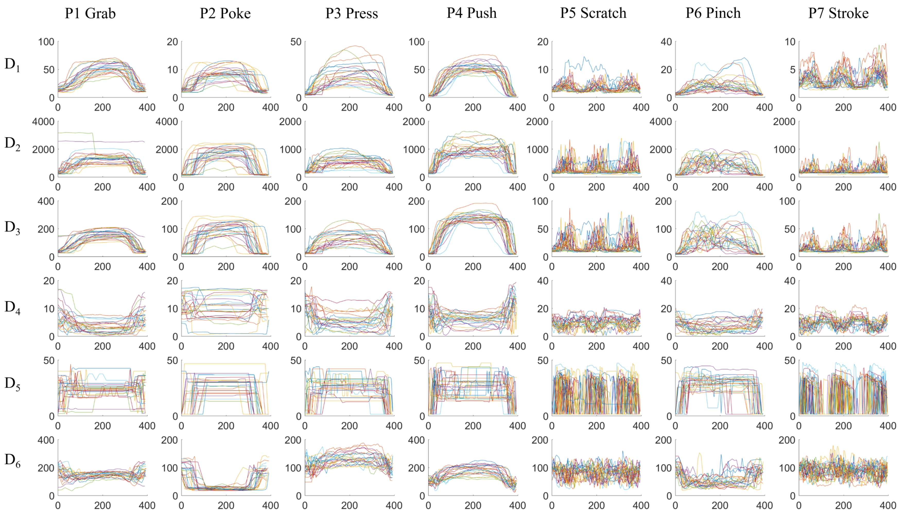
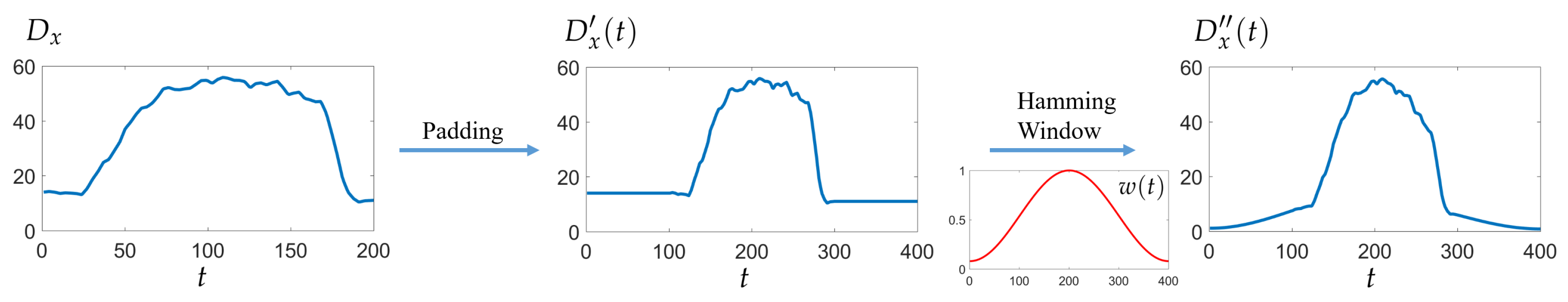
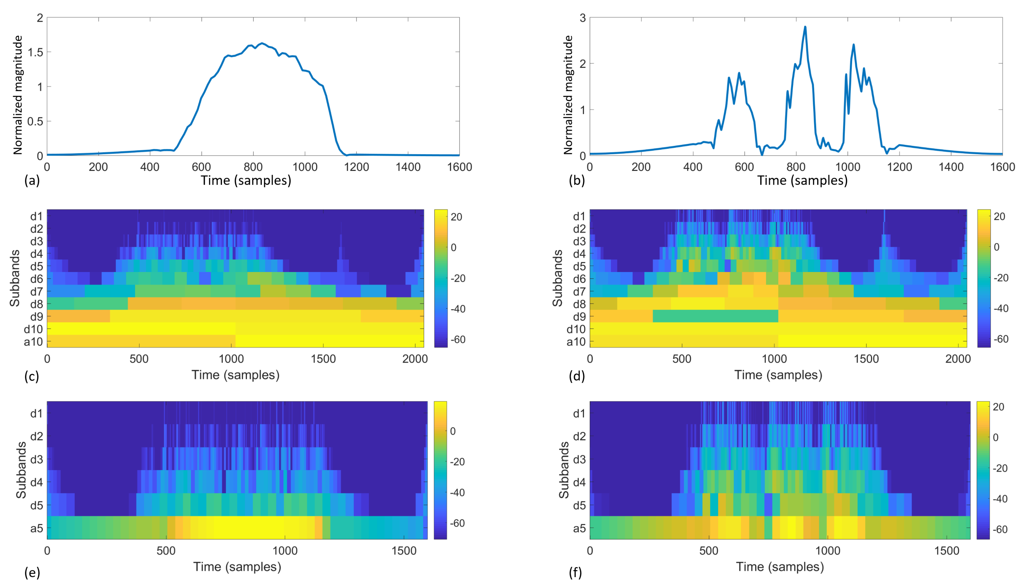
4.1.2. Wavelet Features
4.2. Evaluation Methods
- Medium Tree (maximum 20 splits decision tree)
- Linear Discriminant Analysis (LDA)
- Support Vector Machine (SVM) with linear kernel
- SVM with quadratic kernel
- K-nearest neighbors (KNN) with
- distance weighted KNN with
- Bagged Trees (random forest bag, with decision tree learners)
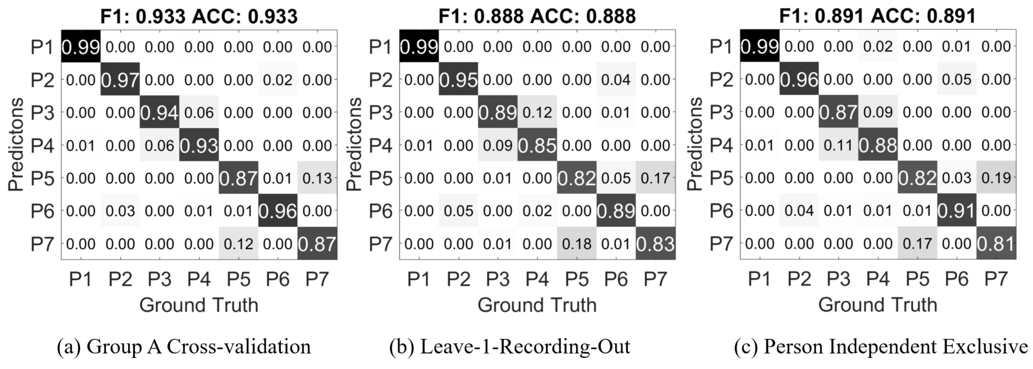
- Random cross-validation: the training data and testing data are from the same data set with k-fold cross-validation.
- Leave one recording out: as the data from the same experiment session may exhibit greater similarity, we use separate different sessions from the same person into training and testing data of the classifier.
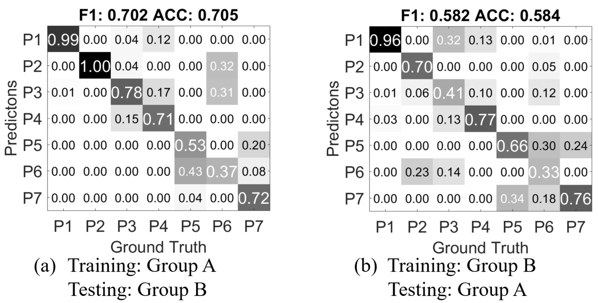
- Person independent exclusive: the training data and testing data are from two groups of persons; the two groups are mutually exclusive. So that the classifier has no previous knowledge of the person being tested.
4.3. Feature Contribution Decomposition
4.3.1. Basic Features
4.3.2. Wavelet Features
4.3.3. Combined Features
4.3.4. Contribution of Different Frame Descriptors
5. Result and Discussion
6. Conclusions and Future Work
Acknowledgments
Author Contributions
Conflicts of Interest
References
- Dario, P.; De Rossi, D. Tactile sensors and the gripping challenge: Increasing the performance of sensors over a wide range of force is a first step toward robotry that can hold and manipulate objects as humans do. IEEE Spectr. 1985, 22, 46–53. [Google Scholar] [CrossRef]
- Yamada, D.; Maeno, T.; Yamada, Y. Artificial finger skin having ridges and distributed tactile sensors used for grasp force control. In Proceedings of the 2001 IEEE/RSJ International Conference on Intelligent Robots and Systems, Maui, HI, USA, 29 October–3 November 2001. [Google Scholar]
- Howe, R.D. Tactile sensing and control of robotic manipulation. Adv. Robot. 1993, 8, 245–261. [Google Scholar] [CrossRef]
- Edin, B.B. Quantitative analysis of static strain sensitivity in human mechanoreceptors from hairy skin. J. Neurophysiol. 1992, 67, 1105–1113. [Google Scholar] [PubMed]
- Hertenstein, M.J.; Keltner, D.; App, B.; Bulleit, B.A.; Jaskolka, A.R. Touch communicates distinct emotions. Emotion 2006, 6, 528. [Google Scholar] [CrossRef] [PubMed]
- Darwin, C. The Expression of the Emotions in Man and Animals; Oxford University Press: Cary, NC, USA, 1998. [Google Scholar]
- Hertenstein, M.J.; Holmes, R.; McCullough, M.; Keltner, D. The communication of emotion via touch. Emotion 2009, 9, 566. [Google Scholar] [CrossRef] [PubMed]
- Wallbott, H.G. Bodily expression of emotion. Eur. J. Soc. Psychol. 1998, 28, 879–896. [Google Scholar] [CrossRef]
- Andreasson, R.; Alenljung, B.; Billing, E.; Lowe, R. Affective Touch in Human-Robot Interaction: Conveying Emotion to the Nao Robot. Int. J. Soc. Robot. accepted for publication.
- Alenljung, B.; Andreasson, R.; Billing, E.A.; Lindblom, J.; Lowe, R. User Experience of Conveying Emotions by Touch. In Proceedings of the IEEE International Symposium on Robot and Human Interactive Communication (RO-MAN), Lisbon, Portugal, 28 August–1 September 2017; pp. 1240–1247. [Google Scholar]
- Cooney, M.D.; Nishio, S.; Ishiguro, H. Recognizing affection for a touch-based interaction with a humanoid robot. In Proceedings of the 2012 IEEE/RSJ International Conference on Intelligent Robots and Systems (IROS), Vilamoura, Portugal, 7–12 October 2012; pp. 1420–1427. [Google Scholar]
- Miwa, H. Effective emotional expressions with emotion expression humanoid robot WE-4RII: Integration of humanoid robot hand RCH-1. In Proceedings of the 2004 IEEE/RSJ International Conference on Intelligent Robot and Systems (IROS), Sendai, Japan, 28 September–2 October 2004; pp. 2203–2208. [Google Scholar]
- Cannata, G.; Maggiali, M.; Metta, G.; Sandini, G. An embedded artificial skin for humanoid robots. In Proceedings of the 2008 IEEE International Conference on Multisensor Fusion and Integration for Intelligent Systems, Seoul, Korea, 20–22 August 2008; pp. 434–438. [Google Scholar]
- Maggiali, M. Artificial Skin for Humanoid Robots. Ph.D. Thesis, University of Genova, Genova, Italy, 2008. [Google Scholar]
- Mittendorfer, P.; Yoshida, E.; Cheng, G. Realizing whole-body tactile interactions with a self-organizing, multi-modal artificial skin on a humanoid robot. Adv. Robot. 2015, 29, 51–67. [Google Scholar] [CrossRef]
- Mazzei, D.; De Maria, C.; Vozzi, G. Touch sensor for social robots and interactive objects affective interaction. Sens. Actuators A 2016, 251, 92–99. [Google Scholar] [CrossRef]
- Lowe, R.; Andreasson, R.; Alenljung, B.; Billing, E. A Wearable Affective Interface for the Nao robot: A Study of Emotion Conveyance by Touch. IEEE Trans. Affect. Comput. 2017. submitted. [Google Scholar]
- Knight, H.; Toscano, R.; Stiehl, W.D.; Chang, A.; Wang, Y.; Breazeal, C. Real-time social touch gesture recognition for sensate robots. In Proceedings of the IEEE/RSJ International Conference on Intelligent Robots and Systems, St. Louis, MO, USA, 10–15 October 2009; pp. 3715–3720. [Google Scholar]
- Flagg, A.; MacLean, K. Affective touch gesture recognition for a furry zoomorphic machine. In Proceedings of the 7th International Conference on Tangible, Embedded and Embodied Interaction, Barcelona, Spain, 10–13 February 2013; pp. 25–32. [Google Scholar]
- Silvera Tawil, D.; Rye, D.; Velonaki, M. Interpretation of the modality of touch on an artificial arm covered with an EIT-based sensitive skin. Int. J. Robot. Res. 2012, 31, 1627–1641. [Google Scholar] [CrossRef]
- Jung, M.M.; Poel, M.; Poppe, R.; Heylen, D.K. Automatic recognition of touch gestures in the corpus of social touch. J. Multimodal User Interfaces 2017, 11, 81–96. [Google Scholar] [CrossRef]
- Zhou, B.; Sundholm, M.; Cheng, J.; Cruz, H.; Lukowicz, P. Never skip leg day: A novel wearable approach to monitoring gym leg exercises. In Proceedings of the 2016 IEEE International Conference on Pervasive Computing and Communications (PerCom), Sydney, Australia, 14 March 2016; pp. 1–9. [Google Scholar]
- Zhou, B.; Singh, M.S.; Yildirim, M.; Prifti, I.; Zurian, H.C.; Yuncosa, Y.M.; Lukowicz, P. Smart Blanket: A Real-Time User Posture Sensing Approach for Ergonomic Designs. In International Conference on Applied Human Factors and Ergonomics; Springer: Berlin/Heidelberg, Germany, 2017; pp. 193–204. [Google Scholar]
- SimpleSkin. Available online: http://www.simpleskin.org/ (accessed on 11 November 2017).
- Sefar AG. Available online: http://www.sefar.com/ (accessed on 11 November 2017).
- Zhou, B.; Bahle, G.; Fuerg, L.; Singh, M.; Cruz, H.; Lukowicz, P. TRAINWEAR: A Real-Time Assisted Training Feedback System with Fabric Wearable Sensors. In Proceedings of the IEEE International Conference on Pervasive Computing and Communications, Kona, HI, USA, 13–17 March 2017. [Google Scholar]
- Cheng, J.; Sundholm, M.; Hirsch, M.; Zhou, B.; Palacio, S.; Lukowicz, P. Application exploring of ubiquitous pressure sensitive matrix as input resource for home-service robots. In Robot Intelligence Technology and Applications 3; Springer: Berlin/Heidelberg, Germany, 2015; pp. 359–371. [Google Scholar]
- Cirillo, A.; Ficuciello, F.; Natale, C.; Pirozzi, S.; Villani, L. A Conformable Force/Tactile Skin for Physical Human–Robot Interaction. IEEE Robot. Autom. Lett. 2016, 1, 41–48. [Google Scholar] [CrossRef]
- Lee, H.; Park, K.; Kim, Y.; Kim, J. Durable and Repairable Soft Tactile Skin for Physical Human Robot Interaction. In Proceedings of the Companion of the 2017 ACM/IEEE International Conference on Human-Robot Interaction, Vienna, Austria, 6–9 March 2017; pp. 183–184. [Google Scholar]
- Průša, Z.; Søndergaard, P.L.; Holighaus, N.; Wiesmeyr, C.; Balazs, P. The Large Time-Frequency Analysis Toolbox 2.0. In Sound, Music, and Motion; Lecture Notes in Computer Science; Springer International Publishing: Cham, Switzerland, 2013; pp. 419–442. [Google Scholar]
- Mallat, S. A Wavelet Tour of Signal Processing; Academic Press: Cambridge, MA, USA, 1999. [Google Scholar]
- Daubechies, I. Ten Lectures on Wavelets; Society for Industrial and Applied Mathematics: Philadelphia, PA, USA, 1992. [Google Scholar]


| Index | Gesture | Details |
|---|---|---|
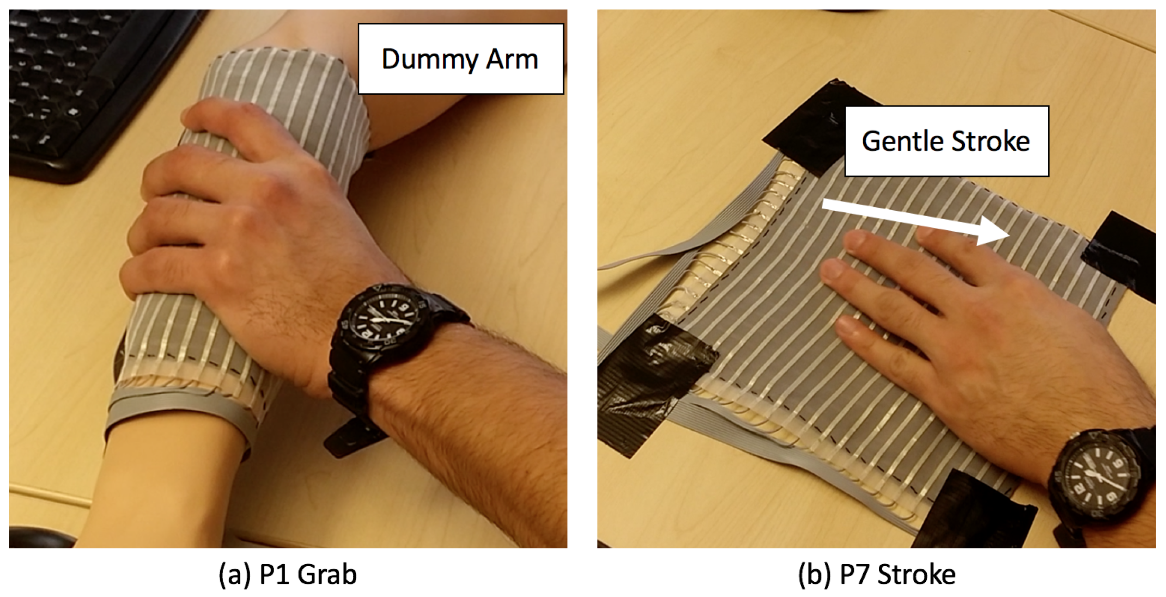
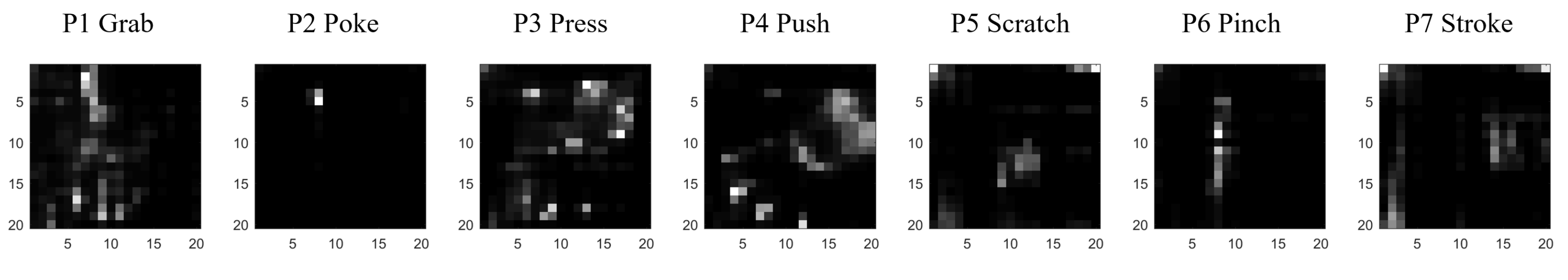
| P1 | grab | whole hand grabbing the dummy’s arm |
| P2 | poke | with one finger, quick and forceful action |
| P3 | press | with multiple finger tips, slow action |
| P4 | push | whole hand including palm, slow action |
| P5 | scratch | with multiple finger tips, quick repeating actions |
| P6 | pinch | on a small area, forceful action |
| P7 | stroke | with multiple fingers, gentle repeating actions |
| Level | Subband Index (j) | Frequency in fn | Frequency in Hz | Coefficients |
|---|---|---|---|---|
| 1 | d1 | fn/2–fn | 25–50 | |
| 2 | d2 | fn/4–fn/2 | 12.5–25 | |
| 3 | d3 | fn/8–fn/2 | 6.25–12.5 | |
| 4 | d4 | fn/16–fn/8 | 3.125–6.25 | |
| 5 | d5 | fn/32–fn/16 | 1.5625–3.125 | |
| 5 | a5 | 0–fn/32 | 0–1.5625 |
| Classifier | ACC |
|---|---|
| Medium Tree | 80.50% |
| LDA | 79.10% |
| SVM (Linear) | 90.80% |
| SVM (Quadratic) | 91.90% |
| KNN () | 86.20% |
| Weighted KNN () | 87.00% |
| Bagged Trees | 89.60% |
| Classifier | ACC () | ACC () | ACC () | ACC () |
|---|---|---|---|---|
| Medium Tree | 82.10% | 79.70% | 78.10% | 77.70% |
| LDA | 75.00% | 77.90% | 74.10% | 77.20% |
| SVM (Linear) | 91.70% | 91.10% | 88.50% | 87.10% |
| SVM (Quadratic) | 92.30% | 92.40% | 89.70% | 87.80% |
| KNN () | 85.40% | 84.30% | 77.50% | 77.00% |
| Weighted KNN () | 86.10% | 84.60% | 77.80% | 77.60% |
| Bagged Trees | 91.60% | 91.00% | 88.00% | 86.60% |
| Classifier | ACC () | ACC () | ACC () | ACC () |
|---|---|---|---|---|
| Medium Tree | 83.80% | 83.70% | 83.20% | 81.20% |
| LDA | 80.20% | 82.30% | 81.20% | 83.60% |
| SVM (Linear) | 92.80% | 92.70% | 92.10% | 91.70% |
| SVM (Quadratic) | 93.30% | 93.60% | 92.80% | 92.20% |
| KNN () | 87.10% | 86.90% | 84.00% | 86.00% |
| Weighted KNN () | 87.70% | 87.20% | 83.90% | 86.00% |
| Bagged Trees | 92.40% | 92.30% | 91.50% | 90.80% |
| Classifier | ACC () | ACC () | ACC () | ACC () | ACC () |
|---|---|---|---|---|---|
| Medium Tree | 70.90% | 70.50% | 71.40% | 74.30% | 83.80% |
| LDA | 68.80% | 67.70% | 64.50% | 73.00% | 80.20% |
| SVM (Linear) | 85.80% | 83.40% | 85.20% | 85.00% | 92.80% |
| SVM (Quadratic) | 88.00% | 84.60% | 86.10% | 85.30% | 93.30% |
| KNN () | 74.90% | 73.70% | 73.10% | 78.80% | 87.10% |
| Weighted KNN () | 75.50% | 74.70% | 74.10% | 79.10% | 87.70% |
| Bagged Trees | 84.90% | 82.50% | 83.10% | 85.00% | 92.40% |
© 2017 by the authors. Licensee MDPI, Basel, Switzerland. This article is an open access article distributed under the terms and conditions of the Creative Commons Attribution (CC BY) license (http://creativecommons.org/licenses/by/4.0/).
Share and Cite
Zhou, B.; Altamirano, C.A.V.; Zurian, H.C.; Atefi, S.R.; Billing, E.; Martinez, F.S.; Lukowicz, P. Textile Pressure Mapping Sensor for Emotional Touch Detection in Human-Robot Interaction. Sensors 2017, 17, 2585. https://doi.org/10.3390/s17112585
Zhou B, Altamirano CAV, Zurian HC, Atefi SR, Billing E, Martinez FS, Lukowicz P. Textile Pressure Mapping Sensor for Emotional Touch Detection in Human-Robot Interaction. Sensors. 2017; 17(11):2585. https://doi.org/10.3390/s17112585
Chicago/Turabian StyleZhou, Bo, Carlos Andres Velez Altamirano, Heber Cruz Zurian, Seyed Reza Atefi, Erik Billing, Fernando Seoane Martinez, and Paul Lukowicz. 2017. "Textile Pressure Mapping Sensor for Emotional Touch Detection in Human-Robot Interaction" Sensors 17, no. 11: 2585. https://doi.org/10.3390/s17112585
APA StyleZhou, B., Altamirano, C. A. V., Zurian, H. C., Atefi, S. R., Billing, E., Martinez, F. S., & Lukowicz, P. (2017). Textile Pressure Mapping Sensor for Emotional Touch Detection in Human-Robot Interaction. Sensors, 17(11), 2585. https://doi.org/10.3390/s17112585