
Object Detection and Classification by Decision-Level Fusion for Intelligent Vehicle Systems


Abstract
:1. Introduction
2. Related Work
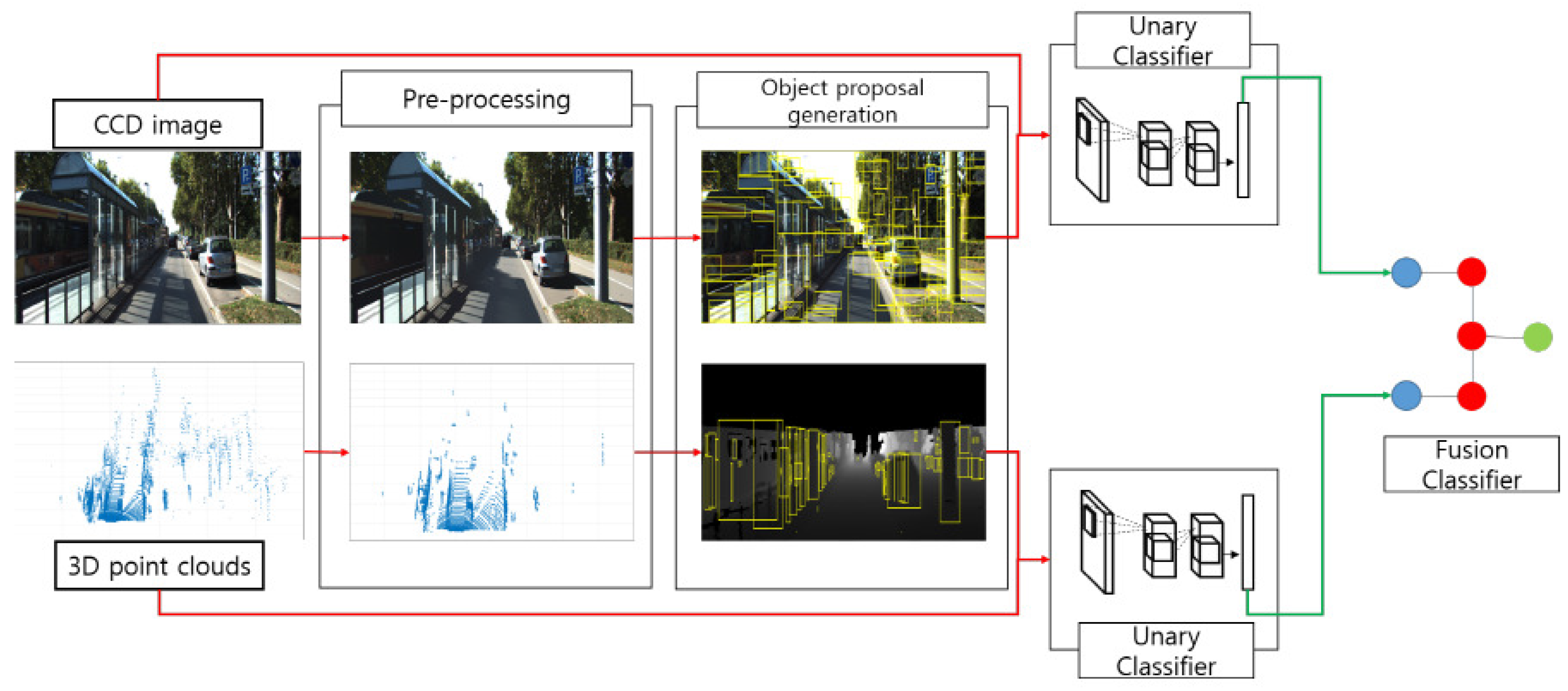
3. Overview
4. Pre-Processing
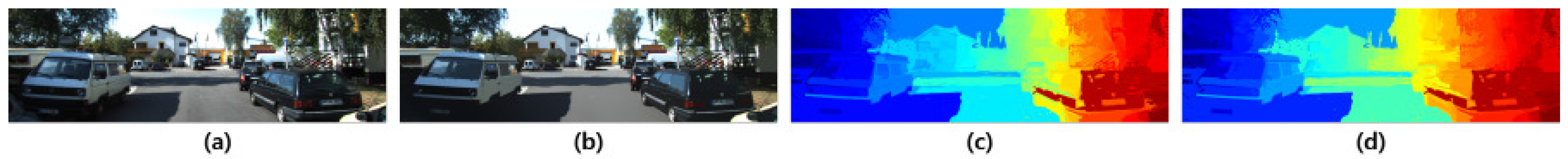
4.1. Norm-Based Color Flattening
| Algorithm 1 Split Bregman for color-flattening. |
|
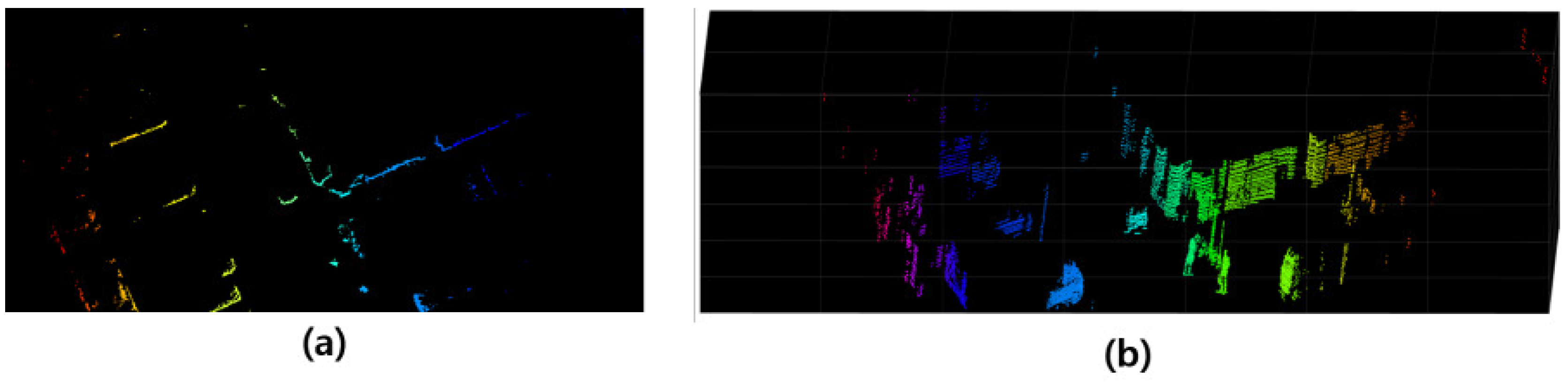
4.2. The 3D Occupancy Voxel Spaces
5. Object-Region Proposal Generation
5.1. Object-Region Proposal from the CCD Sensor
5.2. Object-Region Proposal from the LiDAR Sensor
6. Classifying Object-Region Proposals
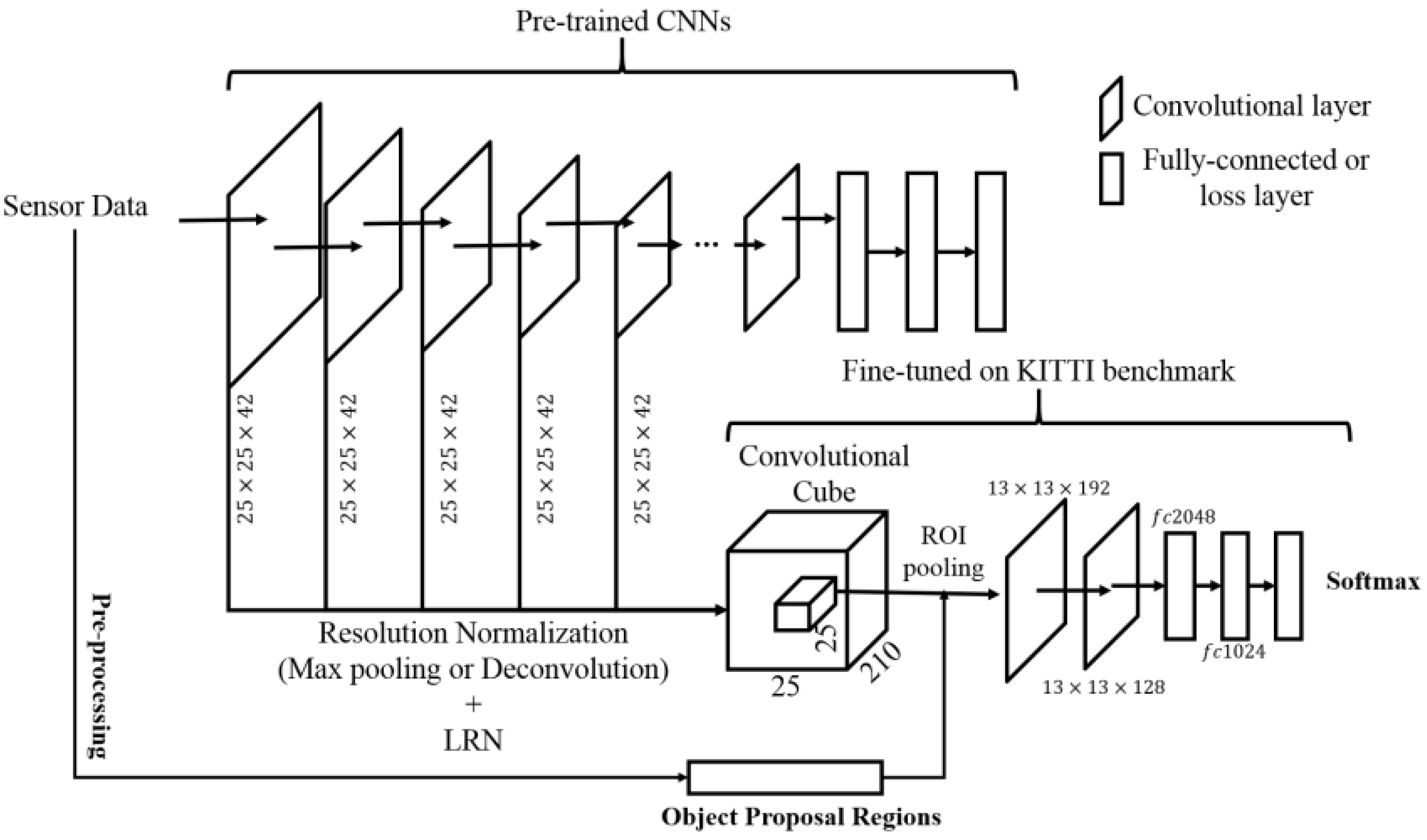
6.1. Unary Classifier
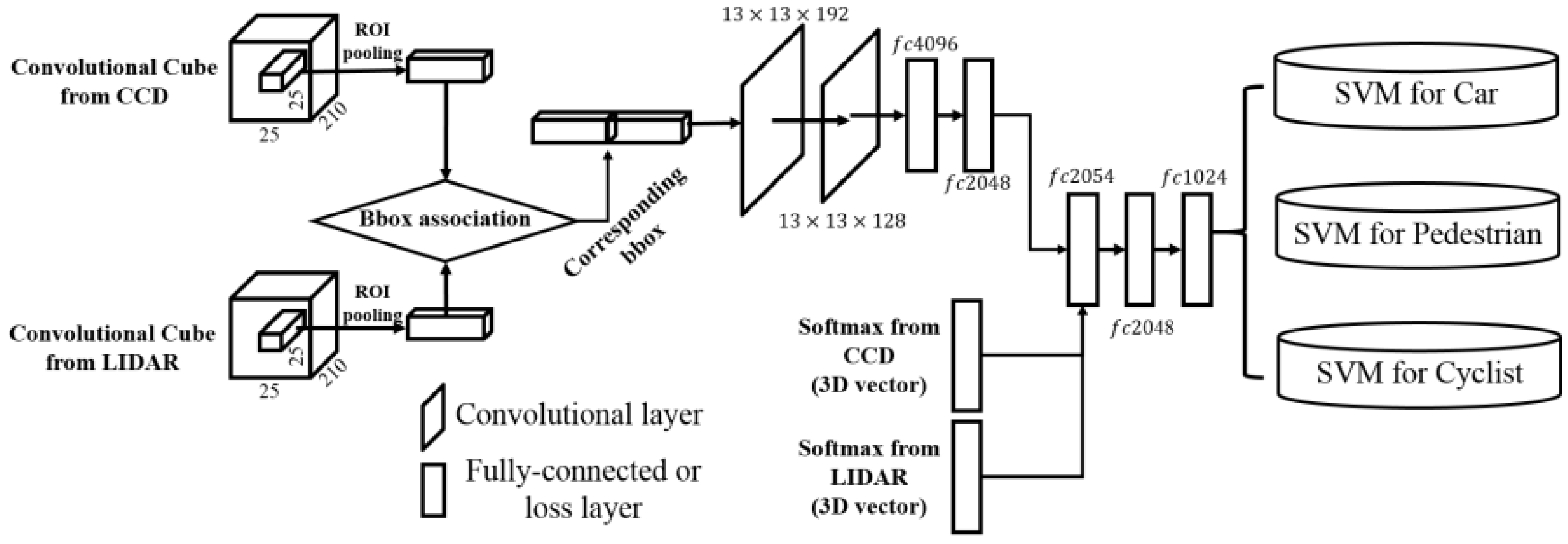
6.2. Fusion Classifier
7. Experimental Results
7.1. Setup
7.2. Evaluation
8. Conclusions and Future Works
Acknowledgments
Author Contributions
Conflicts of Interest
References
- Dalal, N.; Triggs, B. Histograms of oriented gradients for human detection. In Proceedings of the 2005 IEEE Computer Society Conference on Computer Vision and Pattern Recognition (CVPR’05), Los Alamitos, CA, USA, 20–25 June 2005; Volume 1, pp. 886–893.
- Bouzouraa, M.E.; Hofmann, U. Fusion of occupancy grid mapping and model based object tracking for driver assistance systems using laser and radar sensors. In Proceedings of the 2010 IEEE Intelligent Vehicles Symposium (IV), La Jolla, CA, USA, 21–24 June 2010; pp. 294–300.
- Nuss, D.; Wilking, B.; Wiest, J.; Deusch, H.; Reuter, S.; Dietmayer, K. Decision-free true positive estimation with grid maps for multi-object tracking. In Proceedings of the 16th International IEEE Conference on Intelligent Transportation Systems (ITSC 2013), The Hague, The Netherlands, 6–9 October 2013; pp. 28–34.
- Suykens, J.A.; Vandewalle, J. Least squares support vector machine classifiers. Neural Process. Lett. 1999, 9, 293–300. [Google Scholar] [CrossRef]
- Viola, P.; Jones, M. Fast and robust classification using asymmetric adaboost and a detector cascade. Adv. Neural Inf. Process. Syst. 2001, 2, 1311–1318. [Google Scholar]
- Papon, J.; Abramov, A.; Schoeler, M.; Worgotter, F. Voxel cloud connectivity segmentation-supervoxels for point clouds. In Proceedings of the IEEE Conference on Computer Vision and Pattern Recognition, Portland, OR, USA, 23–28 June 2013; pp. 2027–2034.
- Himmelsbach, M.; Luettel, T.; Wuensche, H.J. Real-time object classification in 3D point clouds using point feature histograms. In Proceedings of the 2009 IEEE/RSJ International Conference on Intelligent Robots and Systems, St. Louis, MO, USA, 11–15 October 2009; pp. 994–1000.
- Bi, S.; Han, X.; Yu, Y. An L1 image transform for edge-preserving smoothing and scene-level intrinsic decomposition. ACM Trans. Graph. 2015, 34, 78. [Google Scholar] [CrossRef]
- Geiger, A.; Lenz, P.; Stiller, C.; Urtasun, R. Vision meets robotics: The KITTI dataset. Int. J. Robot. Res. 2013, 32, 1231–1237. [Google Scholar] [CrossRef]
- Rowley, H.A.; Baluja, S.; Kanade, T. Neural network-based face detection. IEEE Trans. Pattern Anal. Mach. Intell. 1998, 20, 23–38. [Google Scholar] [CrossRef]
- Osuna, E.; Freund, R.; Girosit, F. Training support vector machines: An application to face detection. In Proceedings of the IEEE Computer Society Conference on Computer Vision and Pattern Recognition, San Juan, Puerto Rico, 17–19 June 1997; pp. 130–136.
- Hsu, R.L.; Abdel-Mottaleb, M.; Jain, A.K. Face detection in color images. IEEE Trans. Pattern Anal. Mach. Intell. 2002, 24, 696–706. [Google Scholar]
- Oren, M.; Papageorgiou, C.; Sinha, P.; Osuna, E.; Poggio, T. Pedestrian detection using wavelet templates. In Proceedings of the IEEE Computer Society Conference on Computer Vision and Pattern Recognition, San Juan, Puerto Rico, 17–19 June 1997; pp. 193–199.
- Gavrila, D.M. Pedestrian detection from a moving vehicle. In European Conference on Computer Vision; Springer: Berlin, Germany, 2000; pp. 37–49. [Google Scholar]
- Zhao, L.; Thorpe, C.E. Stereo-and neural network-based pedestrian detection. IEEE Trans. Intell. Transp. Syst. 2000, 1, 148–154. [Google Scholar] [CrossRef]
- Nam, W.; Dollár, P.; Han, J.H. Local decorrelation for improved pedestrian detection. Adv. Neural Inf. Process. Syst. 2014, 27, 424–432. [Google Scholar]
- Yan, J.; Zhang, X.; Lei, Z.; Liao, S.; Li, S.Z. Robust multi-resolution pedestrian detection in traffic scenes. In Proceedings of the IEEE Conference on Computer Vision and Pattern Recognition, Portland, OR, USA, 23–28 June 2013; pp. 3033–3040.
- Goerick, C.; Noll, D.; Werner, M. Artificial neural networks in real-time car detection and tracking applications. Pattern Recognit. Lett. 1996, 17, 335–343. [Google Scholar] [CrossRef]
- Hinz, S.; Schlosser, C.; Reitberger, J. Automatic car detection in high resolution urban scenes based on an adaptive 3D-model. In Proceedings of the 2nd GRSS/ISPRS Joint Workshop on Remote Sensing and Data Fusion over Urban Areas, Berlin, Germany, 22–23 May 2003; pp. 167–171.
- Alexe, B.; Deselaers, T.; Ferrari, V. Measuring the objectness of image windows. IEEE Trans. Pattern Anal. Mach. Intell. 2012, 34, 2189–2202. [Google Scholar] [CrossRef] [PubMed]
- Endres, I.; Hoiem, D. Category independent object proposals. In European Conference on Computer Vision; Springer: Berlin, Germany, 2010; pp. 575–588. [Google Scholar]
- Carreira, J.; Sminchisescu, C. Cpmc: Automatic object segmentation using constrained parametric min-cuts. IEEE Trans. Pattern Anal. Mach. Intell. 2012, 34, 1312–1328. [Google Scholar] [CrossRef] [PubMed]
- Uijlings, J.R.; van de Sande, K.E.; Gevers, T.; Smeulders, A.W. Selective search for object recognition. Int. J. Comput. Vis. 2013, 104, 154–171. [Google Scholar] [CrossRef]
- Zitnick, C.L.; Dollár, P. Edge boxes: Locating object proposals from edges. In European Conference on Computer Vision; Springer: Berlin, Germany, 2014; pp. 391–405. [Google Scholar]
- Cheng, M.M.; Zhang, Z.; Lin, W.Y.; Torr, P. BING: Binarized normed gradients for objectness estimation at 300fps. In Proceedings of the IEEE Conference on Computer Vision and Pattern Recognition, Columbus, OH, USA, 23–28 June 2014; pp. 3286–3293.
- Arbeláez, P.; Pont-Tuset, J.; Barron, J.T.; Marques, F.; Malik, J. Multiscale combinatorial grouping. In Proceedings of the Conference on Computer Vision and Pattern Recognition, Columbus, OH, USA, 23–28 June 2014; pp. 328–335.
- Guo, J.M.; Hsia, C.H.; Liu, Y.F.; Shih, M.H.; Chang, C.H.; Wu, J.Y. Fast background subtraction based on a multilayer codebook model for moving object detection. IEEE Trans. Circ. Syst. Video Technol. 2013, 23, 1809–1821. [Google Scholar] [CrossRef]
- Huang, S.C.; Chen, B.H. Automatic moving object extraction through a real-world variable-bandwidth network for traffic monitoring systems. IEEE Trans. Ind. Electr. 2014, 61, 2099–2112. [Google Scholar] [CrossRef]
- Chen, B.H.; Huang, S.C. Probabilistic neural networks based moving vehicles extraction algorithm for intelligent traffic surveillance systems. Inf. Sci. 2015, 299, 283–295. [Google Scholar] [CrossRef]
- Cheng, F.C.; Chen, B.H.; Huang, S.C. A hybrid background subtraction method with background and foreground candidates detection. ACM Trans. Intell. Syst. Technol. 2015, 7, 7. [Google Scholar] [CrossRef]
- Krizhevsky, A.; Sutskever, I.; Hinton, G.E. Imagenet classification with deep convolutional neural networks. Adv. Neural Inf. Process. Syst. 2012, 25, 1097–1105. [Google Scholar]
- Girshick, R.; Donahue, J.; Darrell, T.; Malik, J. Rich feature hierarchies for accurate object detection and semantic segmentation. In Proceedings of the IEEE Conference on Computer Vision and Pattern Recognition, Columbus, OH, USA, 23–28 June 2014; pp. 580–587.
- Kong, T.; Yao, A.; Chen, Y.; Sun, F. HyperNet: Towards Accurate Region Proposal Generation and Joint Object Detection. arXiv 2016. [Google Scholar]
- Ren, S.; He, K.; Girshick, R.B.; Sun, J. Faster R-CNN: Towards Real-Time Object Detection with Region Proposal Networks. arXiv 2015. [Google Scholar] [CrossRef] [PubMed]
- Redmon, J.; Divvala, S.; Girshick, R.; Farhadi, A. You only look once: Unified, real-time object detection. arXiv 2015. [Google Scholar]
- Henry, P.; Krainin, M.; Herbst, E.; Ren, X.; Fox, D. RGB-D mapping: Using depth cameras for dense 3D modeling of indoor environments. In Proceedings of the 12th International Symposium on Experimental Robotics (ISER. Citeseer), New Delhi and Agra, India, 18–21 December 2010.
- Gupta, S.; Arbelaez, P.; Malik, J. Perceptual organization and recognition of indoor scenes from RGB-D images. In Proceedings of the IEEE Conference on Computer Vision and Pattern Recognition, Portland, OR, USA, 23–28 June 2013; pp. 564–571.
- Munera, E.; Poza-Lujan, J.L.; Posadas-Yagüe, J.L.; Simó-Ten, J.E.; Noguera, J.F.B. Dynamic reconfiguration of a rgbd sensor based on qos and qoc requirements in distributed systems. Sensors 2015, 15, 18080–18101. [Google Scholar] [CrossRef] [PubMed]
- Adarve, J.D.; Perrollaz, M.; Makris, A.; Laugier, C. Computing occupancy grids from multiple sensors using linear opinion pools. In Proceedings of the 2012 IEEE International Conference on Robotics and Automation (ICRA), St. Paul, MN, USA, 14–18 May 2012; pp. 4074–4079.
- Oh, S.I.; Kang, H.B. Fast Occupancy Grid Filtering Using Grid Cell Clusters From LiDAR and Stereo Vision Sensor Data. IEEE Sens. J. 2016, 16, 7258–7266. [Google Scholar] [CrossRef]
- González, A.; Villalonga, G.; Xu, J.; Vázquez, D.; Amores, J.; López, A.M. Multiview random forest of local experts combining rgb and LiDAR data for pedestrian detection. In Proceedings of the 2015 IEEE Intelligent Vehicles Symposium (IV), Seoul, Korea, 28 June–1 July 2015; pp. 356–361.
- Nuss, D.; Yuan, T.; Krehl, G.; Stuebler, M.; Reuter, S.; Dietmayer, K. Fusion of laser and radar sensor data with a sequential Monte Carlo Bayesian occupancy filter. In Proceedings of the 2015 IEEE Intelligent Vehicles Symposium (IV), Seoul, Korea, 28 June–1 July 2015; pp. 1074–1081.
- Cho, H.; Seo, Y.W.; Kumar, B.V.; Rajkumar, R.R. A multi-sensor fusion system for moving object detection and tracking in urban driving environments. In Proceedings of the 2014 IEEE International Conference on Robotics and Automation (ICRA), Hong Kong, China, 31 May–7 June 2014; pp. 1836–1843.
- Cadena, C.; Košecká, J. Semantic segmentation with heterogeneous sensor coverages. In Proceedings of the 2014 IEEE International Conference on Robotics and Automation (ICRA), Hong Kong, China, 31 May–7 June 2014; pp. 2639–2645.
- Russell, C.; Kohli, P.; Torr, P.H.; Torr, P.H.S. Associative hierarchical crfs for object class image segmentation. In Proceedings of the 2009 IEEE 12th International Conference on Computer Vision, Kyoto, Japan, 27 September–4 October 2009; pp. 739–746.
- Chavez-Garcia, R.O.; Aycard, O. Multiple sensor fusion and classification for moving object detection and tracking. IEEE Trans. Intell. Transp. Syst. 2016, 17, 525–534. [Google Scholar] [CrossRef]
- Elouedi, Z.; Mellouli, K.; Smets, P. Assessing sensor reliability for multisensor data fusion within the transferable belief model. IEEE Trans. Syst. Man Cybern. Part B Cybern. 2004, 34, 782–787. [Google Scholar] [CrossRef]
- Goldstein, T.; Osher, S. The split Bregman method for L1-regularized problems. SIAM J. Imag. Sci. 2009, 2, 323–343. [Google Scholar] [CrossRef]
- Everingham, M.; Van Gool, L.; Williams, C.K.; Winn, J.; Zisserman, A. The PASCAL visual object classes (VOC) challenge. Int. J. Comput. Vis. 2010, 88, 303–338. [Google Scholar] [CrossRef]
- Smets, P.; Kennes, R. The transferable belief model. Artif. Intell. 1994, 66, 191–234. [Google Scholar] [CrossRef]
- Smets, P. Decision making in the TBM: The necessity of the pignistic transformation. Int. J. Approx. Reason. 2005, 38, 133–147. [Google Scholar] [CrossRef]
- Yager, R.R. On the Dempster-Shafer framework and new combination rules. Inf. Sci. 1987, 41, 93–137. [Google Scholar] [CrossRef]
- Jia, Y.; Shelhamer, E.; Donahue, J.; Karayev, S.; Long, J.; Girshick, R.; Guadarrama, S.; Darrell, T. Caffe: Convolutional architecture for fast feature embedding. In Proceedings of the 22nd ACM international conference on Multimedia, ACM, Orlando, FL, USA, 3–7 November 2014; pp. 675–678.
- Simonyan, K.; Zisserman, A. Very deep convolutional networks for large-scale image recognition. arXiv 2014. [Google Scholar]
- Gupta, S.; Hoffman, J.; Malik, J. Cross modal distillation for supervision transfer. arXiv 2015. [Google Scholar]
- Felzenszwalb, P.F.; Girshick, R.B.; McAllester, D.; Ramanan, D. Object detection with discriminatively trained part-based models. IEEE Trans. Pattern Anal. Mach. Intell. 2010, 32, 1627–1645. [Google Scholar] [CrossRef] [PubMed]
- McCallum, A.; Bellare, K.; Pereira, F. A conditional random field for discriminatively-trained finite-state string edit distance. arXiv 2012. [Google Scholar]
- Chen, X.; Kundu, K.; Zhu, Y.; Berneshawi, A.G.; Ma, H.; Fidler, S.; Urtasun, R. 3D object proposals for accurate object class detection. Adv. Neural Inf. Process. Syst. 2015, 28, 424–432. [Google Scholar]
- Wang, D.Z.; Posner, I. Voting for Voting in Online Point Cloud Object Detection. In Proceedings of the Robotics: Science and Systems, Rome, Italy, 13–17 July 2015.
- Geiger, A.; Wojek, C.; Urtasun, R. Joint 3D Estimation of Objects and Scene Layout; NIPS: Granada, Spain, 2011. [Google Scholar]
- Benenson, R.; Mathias, M.; Tuytelaars, T.; Van Gool, L. Seeking the Strongest Rigid Detector; CVPR: Portland, OR, USA, 2013. [Google Scholar]
- Felzenszwalb, P.F.; Girshick, R.B.; McAllester, D.; Ramanan, D. Object Detection with Discriminatively Trained Part-Based Models. PAMI 2010, 32, 1627–1645. [Google Scholar] [CrossRef] [PubMed]
- Yebes, J.J.; Bergasa, L.M.; García-Garrido, M. Visual Object Recognition with 3D-Aware Features in KITTI Urban Scenes. Sensors 2015, 15, 9228–9250. [Google Scholar] [CrossRef] [PubMed]
- Pepik, B.; Stark, M.; Gehler, P.; Schiele, B. Multi-view and 3D Deformable Part Models. IEEE Trans. Pattern Anal. Mach. Intell. 2015, 37, 2232–2245. [Google Scholar] [CrossRef] [PubMed]
- Pepik, B.; Stark, M.; Gehler, P.; Schiele, B. Occlusion Patterns for Object Class Detection. In Proceedings of the IEEE Conference on Computer Vision and Pattern Recognition (CVPR), Portland, OR, USA, 23–28 June 2013.
- Wu, T.; Li, B.; Zhu, S. Learning And-Or Models to Represent Context and Occlusion for Car Detection and Viewpoint Estimation. arXiv 2015. [Google Scholar] [CrossRef] [PubMed]
- Ohn-Bar, E.; Trivedi, M.M. Learning to Detect Vehicles by Clustering Appearance Patterns. arXiv 2015. [Google Scholar] [CrossRef]
- Xu, J.; Ramos, S.; Vázquez, D.; López, A.M. Hierarchical adaptive structural svm for domain adaptation. arXiv 2014. [Google Scholar] [CrossRef]
- Zhang, S.; Benenson, R.; Schiele, B. Filtered channel features for pedestrian detection. In Proceedings of the 2015 IEEE Conference on Computer Vision and Pattern Recognition (CVPR), Boston, MA, USA, 7–12 June 2015; pp. 1751–1760.
- Paisitkriangkrai, S.; Shen, C.; van den Hengel, A. Pedestrian detection with spatially pooled features and structured ensemble learning. arXiv 2014. [Google Scholar] [CrossRef] [PubMed]
- Xiang, Y.; Choi, W.; Lin, Y.; Savarese, S. Data-Driven 3D Voxel Patterns for Object Category Recognition. In Proceedings of the IEEE Conference on Computer Vision and Pattern Recognition, Boston, MA, USA, 7–12 June 2015.
- Wang, X.; Yang, M.; Zhu, S.; Lin, Y. Regionlets for Generic Object Detection. IEEE Trans. Pattern Anal. Machine Intell. 2015, 37, 2071–2084. [Google Scholar] [CrossRef] [PubMed]
- Premebida, C.; Carreira, J.; Batista, J.; Nunes, U. Pedestrian detection combining rgb and dense LiDAR data. In Proceedings of the 2014 IEEE/RSJ International Conference on Intelligent Robots and Systems (IROS 2014), Chicago, IL, USA, 14–18 September 2014; pp. 4112–4117.
- Gonzalez, A.; Villalonga, G.; Xu, J.; Vazquez, D.; Amores, J.; Lopez, A. Multiview Random Forest of Local Experts Combining RGB and LiDAR data for Pedestrian Detection. In Proceedings of the IEEE Intelligent Vehicles Symposium (IV), Seoul, Korea, 28 June–1 July 2015.


| Section | Parameters or Functions | Descriptions |
|---|---|---|
| Energy function to generate color-flattening, . | ||
| Data term of energy function for pixel-wise intrinsic similarity. | ||
| A concatenated vector of all pixel values in transformed image . | ||
| z | A concatenated vector of all pixel values in original image I. | |
| 4.1 | Smoothness term of energy function. | |
| A 3-dimensional vector of the RGB values at pixel position of transformed image . | ||
| Weights to the difference between of pixel position and of the neighboring pixel of . | ||
| A 3-dimensional vector of the CIELab color space of . | ||
| κ | A constant related to the luminance variations. | |
| M | The matrix consists of and . | |
| and | Intermediate variables of the split Bregman method. | |
| , the i-th 3D point data of 3D point clouds. | ||
| 4.2 | The i-th voxel includes the reflected particles with a size of . | |
| The number of voxels in a 3D point cloud. | ||
| The possible number of reflectance particles in voxel . | ||
| A set of segmented partition of the color-flatted image. | ||
| The number of segmented partitions. | ||
| Set of spatially-connected neighborhood partitions of the partition. | ||
| The dissimilarity function to group the adjacent partitions. | ||
| ; the color dissimilarity between the adjacent partitions. | ||
| A weight constant for the color dissimilarity. | ||
| 5.1 | 75-bin color histogram measured from the mean image . | |
| The texture dissimilarity between the adjacent partitions. | ||
| A weight constant for the texture dissimilarity. | ||
| 240-bin SIFT histogram of original image I. | ||
| A threshold value for grouping adjacent partitions. | ||
| S and | The ground truth of the segmented and inferred segmentation images from the proposed method. | |
| The number of training images to find . | ||
| The structural loss between the ground truth and the inferred segmented partition. | ||
| The classification results of each bounding box provided from the image. | ||
| 6.2 | The classification results of each bounding box provided from the 3D point clouds. | |
| The association component between and . |
| Model | Proposal Generator | Representation | Representation Usage | Modality | Fusion Scheme |
|---|---|---|---|---|---|
| Sliding Window | VGG16 | ConvCube | CCD + LiDAR | CNN | |
| CIOP | VGG16 | ConvCube | CCD + LiDAR | CNN | |
| Objectness | VGG16 | ConvCube | CCD + LiDAR | CNN | |
| Selective Search | VGG16 | ConvCube | CCD + LiDAR | CNN | |
| CPMC | VGG16 | ConvCube | CCD + LiDAR | CNN | |
| MCG | VGG16 | ConvCube | CCD + LiDAR | CNN | |
| EdgeBox | VGG16 | ConvCube | CCD + LiDAR | CNN | |
| Proposed Generator | AlexNet | ConvCube | CCD + LiDAR | CNN | |
| Proposed Generator | VGG16 | conv1 | CCD + LiDAR | CNN | |
| Proposed Generator | VGG16 | conv5 | CCD + LiDAR | CNN | |
| Proposed Generator | VGG16 | fc7 | CCD + LiDAR | CNN | |
| Proposed Generator | VGG16 | conv5 + fc7 | CCD + LiDAR | CNN | |
| Proposed Generator | VGG16 | ConvCube | CCD | × | |
| Proposed Generator | VGG16 | ConvCube | LiDAR | × | |
| Proposed Generator | VGG16 | ConvCube | CCD + LiDAR | Decision-TBM | |
| Proposed Generator | VGG16 | ConvCube | CCD + LiDAR | Decision-CRF | |
| 3DOP | 3DOP | 3DOP | CCD + LiDAR | Feature-3DOP | |
| Proposed Generator | VGG16 | ConvCube | CCD + LiDAR | CNN |
| Method | Recall | # of Bbox | ||
|---|---|---|---|---|
| Cars | Pedestrians | Cyclists | ||
| Sliding window | 100 | 100 | 100 | |
| CIOP | 64.4 | 59.8 | 59.9 | |
| 66.9 | 60.4 | 60.1 | ||
| Selective search | 70.4 | 66.8 | 68.7 | |
| CPMC | 71.7 | 67.4 | 68.6 | |
| MCG | 76.6 | 78.9 | 74.8 | |
| EdgeBox | 85.2 | 84.3 | 82.5 | |
| Ours (CCD) | 88.4 | 85.4 | 84.8 | |
| Ours (LiDAR) | 71.8 | 63.3 | 64.2 | 70 |
| Ours | 90.8 | 88.7 | 86.5 | 500 |
| Model | Cars | Pedestrians | Cyclists | ||||||
|---|---|---|---|---|---|---|---|---|---|
| Easy | Moderate | Hard | Easy | Moderate | Hard | Easy | Moderate | Hard | |
| 90.98 | 88.64 | 79.88 | 82.84 | 69.55 | 66.42 | 82.12 | 71.48 | 64.55 | |
| 90.7 | 83.67 | 79.78 | 80.54 | 68.07 | 65.23 | 80.86 | 68.59 | 63.54 | |
| 91.34 | 85.28 | 77.42 | 81.71 | 68.54 | 61.19 | 78.21 | 68.77 | 63.77 | |
| 85.88 | 87.74 | 79.01 | 79.59 | 68.45 | 62.66 | 82.65 | 65.12 | 61.38 | |
| 91.39 | 87.78 | 75.7 | 75.25 | 66.35 | 61.27 | 76.24 | 66.93 | 63.39 | |
| 89.42 | 82.94 | 77.1 | 80.94 | 67.93 | 61.58 | 79.07 | 66.67 | 63.27 | |
| 85.68 | 87.82 | 79.57 | 81.53 | 65.02 | 65.94 | 78.67 | 67.89 | 60.81 | |
| 87.43 | 84.44 | 75.42 | 73.2 | 65.28 | 64.55 | 77.51 | 66.74 | 60.15 | |
| 86.29 | 81.26 | 73.52 | 72.86 | 63.04 | 60.31 | 74.69 | 61.30 | 56.16 | |
| 74.87 | 80.98 | 75.85 | 77.57 | 60.61 | 62.79 | 70.12 | 62.49 | 59.21 | |
| 77.00 | 82.37 | 75.50 | 77.54 | 60.43 | 56.30 | 73.37 | 64.23 | 56.84 | |
| 88.59 | 83.08 | 77.30 | 79.17 | 64.54 | 64.34 | 75.69 | 66.35 | 59.58 | |
| 88.84 | 84.77 | 73.81 | 77.92 | 68.81 | 59.33 | 72.60 | 67.32 | 57.21 | |
| 70.32 | 67.97 | 59.62 | 64.96 | 59.29 | 37.28 | 63.45 | 58.34 | 30.22 | |
| 84.25 | 81.66 | 74.48 | 69.49 | 67.81 | 62.14 | 70.81 | 68.11 | 60.25 | |
| 83.48 | 82.71 | 70.55 | 78.34 | 68.97 | 60.38 | 72.84 | 68.42 | 61.01 | |
| 93.04 | 88.64 | 79.1 | 81.78 | 67.47 | 64.7 | 78.39 | 68.94 | 61.37 | |
| 94.88 | 89.34 | 81.42 | 83.71 | 70.84 | 68.67 | 83.95 | 72.98 | 66.47 | |
| Fusion | Sensor | Cars | Pedestrians | Cyclists | |||||||
|---|---|---|---|---|---|---|---|---|---|---|---|
| Easy | Moderate | Hard | Easy | Moderate | Hard | Easy | Moderate | Hard | |||
| Vote3D [59] | × | L | 56.80 | 47.99 | 42.57 | 44.48 | 35.74 | 33.72 | 41.43 | 31.24 | 28.62 |
| LSVM-MDPM [60] | × | C | 68.02 | 56.48 | 44.18 | 47.74 | 39.36 | 35.95 | 35.04 | 27.50 | 26.21 |
| SquaresICF [61] | × | C | - | 57.33 | 44.42 | 40.08 | - | ||||
| MDPM-un-BB [62] | × | C | 71.19 | 62.16 | 48.48 | - | - | ||||
| DPM-C8B1 [63] | × | S | 74.33 | 60.99 | 47.16 | 38.96 | 29.03 | 25.61 | 43.49 | 29.04 | 26.20 |
| DPM-VOC+ VP [64] | × | C | 74.95 | 64.71 | 48.76 | 59.48 | 44.86 | 40.37 | 42.43 | 31.08 | 28.23 |
| OC-DPM [65] | × | C | 74.94 | 65.95 | 53.86 | - | - | ||||
| AOG [66] | × | C | 84.36 | 71.88 | 59.27 | - | - | ||||
| SubCat [67] | × | C | 84.14 | 75.46 | 59.71 | 54.67 | 42.34 | 37.95 | - | ||
| DA-DPM [68] | × | C | - | 56.36 | 45.51 | 41.08 | - | ||||
| Faster R-CNN [34] | × | C | 86.71 | 81.84 | 71.12 | 78.86 | 65.90 | 61.18 | 72.26 | 63.35 | 55.90 |
| FilteredICF [69] | × | C | - | 61.14 | 53.98 | 49.29 | - | ||||
| pAUCEnsT [70] | × | C | - | 65.26 | 54.49 | 48.60 | 51.62 | 38.03 | 33.38 | ||
| 3DVP [71] | × | C | 87.46 | 75.77 | 65.38 | - | - | ||||
| Regionlets [72] | × | C | 84.75 | 76.45 | 59.70 | 73.14 | 61.15 | 55.21 | 70.41 | 58.72 | 51.83 |
| uickitti | × | C | 90.83 | 89.23 | 79.46 | 83.49 | 71.84 | 67.00 | 78.40 | 70.90 | 62.54 |
| Fusion-DPM [73] | Decision | L + C | - | 59.51 | 46.67 | 42.05 | - | ||||
| MV-RGBD-RF [74] | Early | L + C | 76.40 | 69.92 | 57.47 | 73.30 | 56.59 | 49.63 | 52.97 | 42.61 | 37.42 |
| 3DOP [58] | Early | S + C | 93.04 | 88.64 | 79.10 | 81.78 | 67.47 | 64.70 | 78.39 | 68.94 | 61.37 |
| Ours (CCD) | × | C | 88.84 | 84.77 | 73.81 | 77.92 | 68.81 | 59.33 | 72.60 | 67.32 | 57.21 |
| Ours (LiDAR) | × | L | 70.32 | 67.97 | 59.62 | 64.96 | 59.29 | 37.28 | 63.45 | 58.34 | 30.22 |
| Ours (TBM) | Decision | L + C | 84.25 | 81.66 | 74.48 | 69.49 | 67.81 | 62.14 | 70.81 | 68.11 | 60.25 |
| Ours (CRF) | Decision | L + C | 83.48 | 82.71 | 70.55 | 78.34 | 68.97 | 60.38 | 72.84 | 68.42 | 61.01 |
| Ours | Decision | L + C | 94.88 | 89.34 | 81.42 | 83.71 | 70.84 | 68.67 | 83.95 | 72.98 | 66.47 |
© 2017 by the authors; licensee MDPI, Basel, Switzerland. This article is an open access article distributed under the terms and conditions of the Creative Commons Attribution (CC BY) license (http://creativecommons.org/licenses/by/4.0/).
Share and Cite
Oh, S.-I.; Kang, H.-B. Object Detection and Classification by Decision-Level Fusion for Intelligent Vehicle Systems. Sensors 2017, 17, 207. https://doi.org/10.3390/s17010207
Oh S-I, Kang H-B. Object Detection and Classification by Decision-Level Fusion for Intelligent Vehicle Systems. Sensors. 2017; 17(1):207. https://doi.org/10.3390/s17010207
Chicago/Turabian StyleOh, Sang-Il, and Hang-Bong Kang. 2017. "Object Detection and Classification by Decision-Level Fusion for Intelligent Vehicle Systems" Sensors 17, no. 1: 207. https://doi.org/10.3390/s17010207
APA StyleOh, S.-I., & Kang, H.-B. (2017). Object Detection and Classification by Decision-Level Fusion for Intelligent Vehicle Systems. Sensors, 17(1), 207. https://doi.org/10.3390/s17010207