
Maximum Correntropy Unscented Kalman Filter for Spacecraft Relative State Estimation


Abstract
:1. Introduction
2. Preliminaries
2.1. Maximum Correntropy Criterion
2.2. Unscented Kalman Filter
2.2.1. Predict
2.2.2. Update
3. Unscented Kalman Filter under MCC
- Choose a proper kernel bandwidth σ; set an initial estimate and corresponding covariance matrix ; and let ;
4. Illustrative Examples
4.1. Example 1
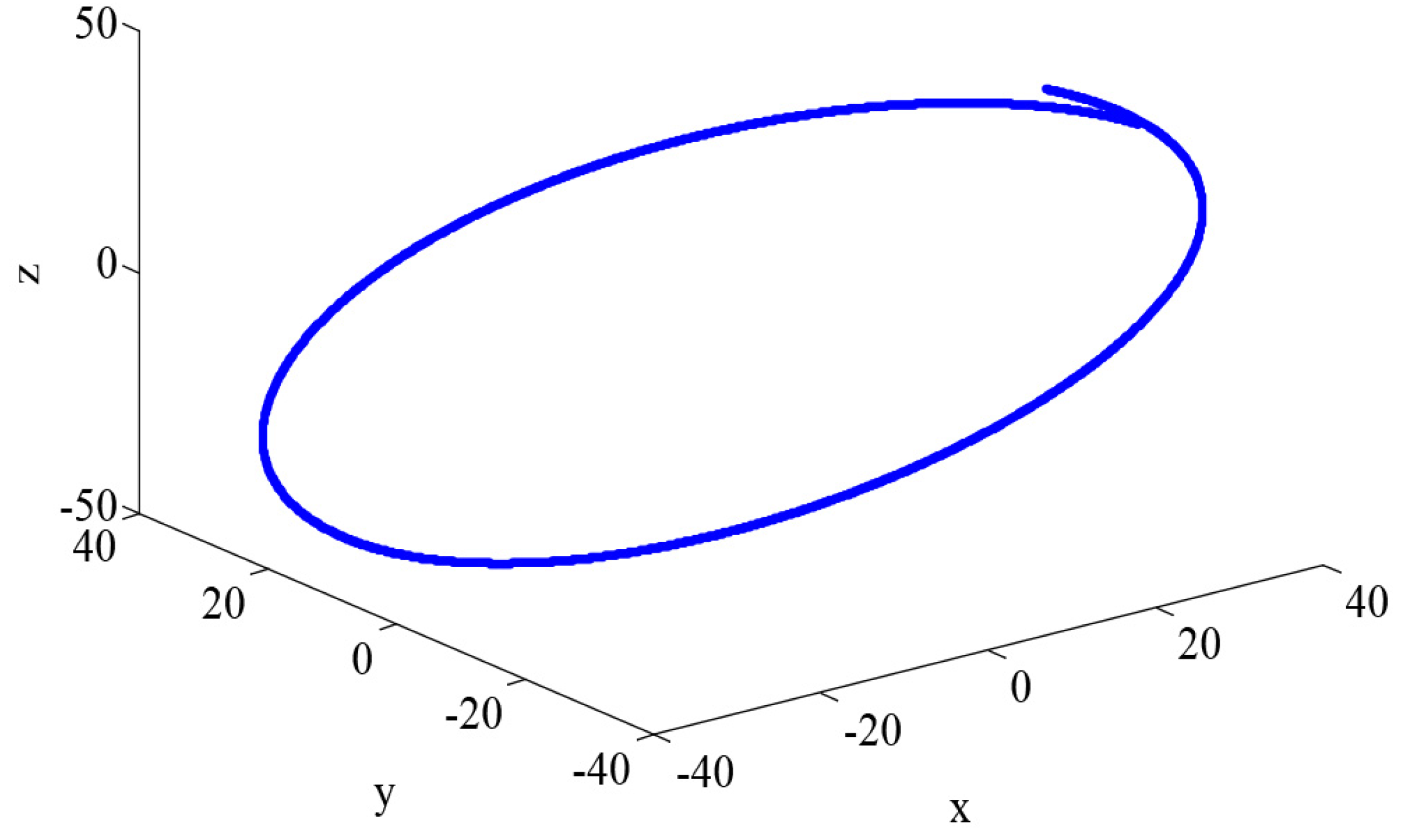
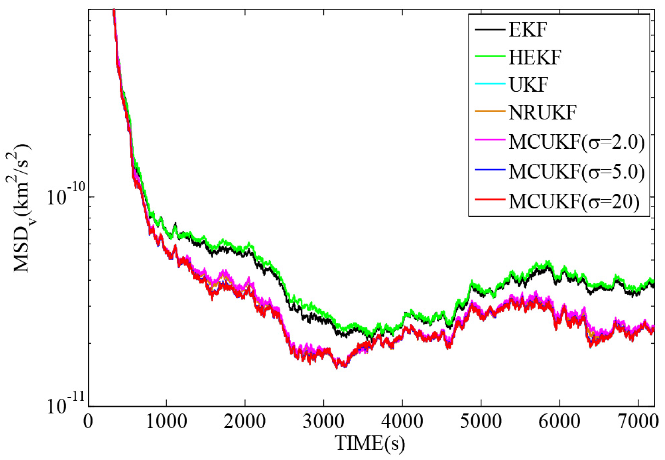
4.2. Example 2
5. Conclusions
Acknowledgments
Author Contributions
Conflicts of Interest
References
- Marszalek, M.; Kurz, O.; Drentschew, M.; Schmidt, M.; Schilling, K. Intersatellite Links and Relative Navigation: Pre-conditions for Formation Flights with Pico- and Nanosatellites. In Proceedings of the 18th IFAC World Congress, Milan, Italy, 29 August–3 September 2011; pp. 3027–3032.
- Liu, X.; Sun, Z.; Zhang, J.; Wu, X. Relative Navigation Method of Communication Supporting Spacecraft base-on Particle Filter. J. Comput. Inf. Syst. 2013, 9, 1–8. [Google Scholar]
- Wu, F.; Sui, X.; Zhao, Y.; Zhang, Y. Relative navigation for formation flying spacecrafts using X-ray pulsars. In Proceedings of the IEEE/ION Position Location and Navigation Symposium (PLANS), Myrtle Beach, SC, USA, 23–26 April 2012; pp. 1289–1292.
- Kelsey, J.; Byrne, J.; Cosgrove, M.; Seereeram, S.; Mehra, R. Vision-based relative pose estimation for autonomous rendezvous and docking. In Proceedings of the IEEE Aerospace Conference, Big Sky, MT, USA, 4–11 March 2006; pp. 1–20.
- Kalman, R.E. A new approach to linear filtering and prediction problems. Trans. ASME-J. Basic Eng. 1960, 82, 35–45. [Google Scholar] [CrossRef]
- Bryson, A.; Ho, Y. Applied Optimal Control: Optimization, Estimation and Control; CRC Press: Boca Raton, FL, USA, 1975. [Google Scholar]
- Nahi, N.E. Estimation Theory and Applications; Wiley: New York, NY, USA, 1969. [Google Scholar]
- Hablani, H.B.; Tapper, M.L.; Dana-Bashian, D.J. Guidance and Relative Navigation for Autonomous Rendezvous in a Circular Orbit. Trans. ASME-J. Basic Eng. 2002, 25, 553–562. [Google Scholar] [CrossRef]
- Baek, K.; Bang, H. Adaptive sparse grid quadrature filter for spacecraft relative navigation. Acta Astronaut. 2013, 87, 96–106. [Google Scholar] [CrossRef]
- Anderson, B.; Moore, J. Optimal Filtering; Prentice-Hall: Englewood Cliffs, NJ, USA, 1979. [Google Scholar]
- Haykin, S. Kalman Filtering and Neural Networks; John Wiley & Sons: New York, NY, USA, 2001. [Google Scholar]
- Simon, D. Optimal State Estimation: Kalman, H∞ and Nonlinear Approaches; John Wiley & Sons: Hoboken, NJ, USA, 2006. [Google Scholar]
- Julier, S.; Uhlmann, J.; Durrant-Whyte, H.F. A new method for the nonlinear transformation of means and covariances in filters and estimators. IEEE Trans. Autom. Control 2000, 45, 477–482. [Google Scholar] [CrossRef]
- Schick, I.; Mitter, S. Robust Recursive Estimation in the Presence of Heavy-Tailed Observation Noise. Ann. Stat. 1994, 22, 1045–1080. [Google Scholar] [CrossRef]
- Huber, P. Robust Statistics; Springer: Berlin, Germany, 2011. [Google Scholar]
- Chang, L.; Hu, B.; Chang, G.; Li, A. Huber-based novel robust unscented Kalman filter. IET Sci. Meas. Technol. 2012, 6, 502–509. [Google Scholar] [CrossRef]
- Principe, J.C. Information Theoretic Learning: Renyi’s Entropy and Kernel Perspectives; Springer: New York, NY, USA, 2010. [Google Scholar]
- Chen, B.; Zhu, Y.; Hu, J.; Principe, J.C. System Parameter Identification: Information Criteria and Algorithms; Newnes: Oxford, UK, 2013. [Google Scholar]
- Liu, W.; Pokharel, P.P.; Principe, J.C. Correntropy: Properties, and applications in non-Gaussian signal processing. IEEE Trans. Signal Process. 2007, 55, 5286–5298. [Google Scholar] [CrossRef]
- Chen, B.; Principe, J.C. Maximum correntropy estimation is a smoothed MAP estimation. IEEE Signal Process. Lett. 2012, 19, 491–494. [Google Scholar] [CrossRef]
- Ma, W.; Qu, H.; Zhao, J. Estimator with Forgetting Factor of Correntropy and Recursive Algorithm for Traffic Network Prediction. In Proceedings of the Chinese Control and Decision Conference (CCDC), Guiyang, China, 25–27 May 2013; pp. 490–494.
- Chen, X.; Yang, J.; Liang, J.; Ye, Q. Recursive robust least squares support vector regression based on maximum correntropy criterion. Neurocomputing 2012, 97, 63–73. [Google Scholar] [CrossRef]
- He, R.; Hu, B.; Yuan, X.; Wang, L. Robust Recognition via Information Theoretic Learning; Springer: Amsterdam, The Netherlands, 2014. [Google Scholar]
- He, R.; Zheng, W.; Hu, B. Maximum correntropy criterion for robust face recognition. IEEE Trans. Pattern Anal. 2011, 33, 1561–1576. [Google Scholar]
- He, R.; Hu, B.; Zheng, W.; Kong, X. Robust principal component analysis based on maximum correntropy criterion. IEEE Trans. Image Process. 2011, 20, 1485–1494. [Google Scholar] [PubMed]
- Chen, L.; Qu, H.; Zhao, J.; Chen, B.; Principe, J.C. Efficient and robust deep learning with Correntropy-induced loss function. Neural Comput. Appl. 2016, 27, 1019–1031. [Google Scholar] [CrossRef]
- Bessa, R.J.; Miranda, V.; Gama, J. Entropy, and correntropy against minimum square error in offline, and online three-day ahead wind power forecasting. IEEE Trans. Power Syst. 2009, 24, 1657–1666. [Google Scholar] [CrossRef]
- Ma, W.; Qu, H.; Gui, G.; Xu, L.; Zhao, J.; Chen, B. Maximum correntropy criterion based sparse adaptive filtering algorithms for robust channel estimation under non-Gaussian environments. J. Frankl. Inst. 2015, 352, 2708–2727. [Google Scholar] [CrossRef]
- Chen, B.; Xing, L.; Liang, J.; Zheng, N.; Principe, J.C. Steady-State Mean-Square Error Analysis for Adaptive Filtering under the Maximum Correntropy Criterion. IEEE Signal Process. Lett. 2014, 21, 880–884. [Google Scholar]
- Shi, L.; Lin, Y. Convex Combination of Adaptive Filters under the Maximum Correntropy Criterion in Impulsive Interference. IEEE Signal Process. Lett. 2014, 21, 1385–1388. [Google Scholar] [CrossRef]
- Chen, B.; Xing, L.; Zhao, H.; Zheng, N.; Principe, J.C. Generalized correntropy for robust adaptive filtering. IEEE Trans. Signal Process. 2016, 64, 3376–3387. [Google Scholar] [CrossRef]
- Chen, B.; Liu, X.; Zhao, H.; Principe, J.C. Maximum Correntropy Kalman Filter. Available online: http://arxiv.org/abs/1509.04580 (accessed on 18 September 2016).
- Liu, X.; Chen, B.; Xu, B.; Wu, Z.; Honeine, P. Maximum Correntropy Unscented Filter. Available online: http://arxiv.org/abs/1608.07526 (accessed on 18 September 2016).
- Chen, B.; Wang, J.; Zhao, H.; Zheng, N.; Principe, J.C. Convergence of a fixed-point algorithm under maximum correntropy criterion. IEEE Signal Process. Lett. 2015, 22, 1723–1727. [Google Scholar] [CrossRef]
- Schaub, H.; Junkins, J.L. Analytical Mechanics of Space Systems; American Institute of Aeronautics and Astronautics Education Series: Reston, VA, USA, 2003. [Google Scholar]
- El-Hawary, F.; Jing, Y. Robust Regression-Based EKF for Tracking Underwater Targets. IEEE J. Ocean. Eng. 1995, 20, 31–41. [Google Scholar] [CrossRef]


| Filter | MSE of x |
|---|---|
| UKF | 67.6974 |
| MCUKF | 87.6836 |
| MCUKF | 80.8406 |
| MCUKF | 74.0286 |
| MCUKF | 72.3362 |
| MCUKF | 68.6795 |
| Filter | MSE of x |
|---|---|
| UKF | 85.8439 |
| MCUKF | 84.1944 |
| MCUKF | 82.6933 |
| MCUKF | 83.1098 |
| MCUKF | 84.7173 |
| MCUKF | 85.4411 |
| Orbital Elements | Chief Spacecraft |
|---|---|
| Semi-major axis | 8000 km |
| Eccentricity | 0.150 |
| Orbit inclination | rad |
| Argument of perigee | rad |
| Right ascension of the ascending node | rad |
| True anomaly | 0 rad |
| Filter | ||
|---|---|---|
| EKF | ||
| HEKF | ||
| UKF | ||
| NRUKF | ||
| MCUKF | ||
| MCUKF | ||
| MCUKF |
| Filter | ||
|---|---|---|
| EKF | ||
| HEKF | ||
| UKF | ||
| NRUKF | ||
| MCUKF | ||
| MCUKF | ||
| MCUKF |
| Filter | Computation Ratio |
|---|---|
| UKF | 1 |
| HEKF | |
| NRUKF | |
| MCUKF |
© 2016 by the authors; licensee MDPI, Basel, Switzerland. This article is an open access article distributed under the terms and conditions of the Creative Commons Attribution (CC-BY) license (http://creativecommons.org/licenses/by/4.0/).
Share and Cite
Liu, X.; Qu, H.; Zhao, J.; Yue, P.; Wang, M. Maximum Correntropy Unscented Kalman Filter for Spacecraft Relative State Estimation. Sensors 2016, 16, 1530. https://doi.org/10.3390/s16091530
Liu X, Qu H, Zhao J, Yue P, Wang M. Maximum Correntropy Unscented Kalman Filter for Spacecraft Relative State Estimation. Sensors. 2016; 16(9):1530. https://doi.org/10.3390/s16091530
Chicago/Turabian StyleLiu, Xi, Hua Qu, Jihong Zhao, Pengcheng Yue, and Meng Wang. 2016. "Maximum Correntropy Unscented Kalman Filter for Spacecraft Relative State Estimation" Sensors 16, no. 9: 1530. https://doi.org/10.3390/s16091530
APA StyleLiu, X., Qu, H., Zhao, J., Yue, P., & Wang, M. (2016). Maximum Correntropy Unscented Kalman Filter for Spacecraft Relative State Estimation. Sensors, 16(9), 1530. https://doi.org/10.3390/s16091530