
Improved Bearings-Only Multi-Target Tracking with GM-PHD Filtering


Abstract
:1. Introduction
2. The Bearings-Only MTT Problem
3. The Proposed GMM-PHD Filter
3.1. Intensity Prediction
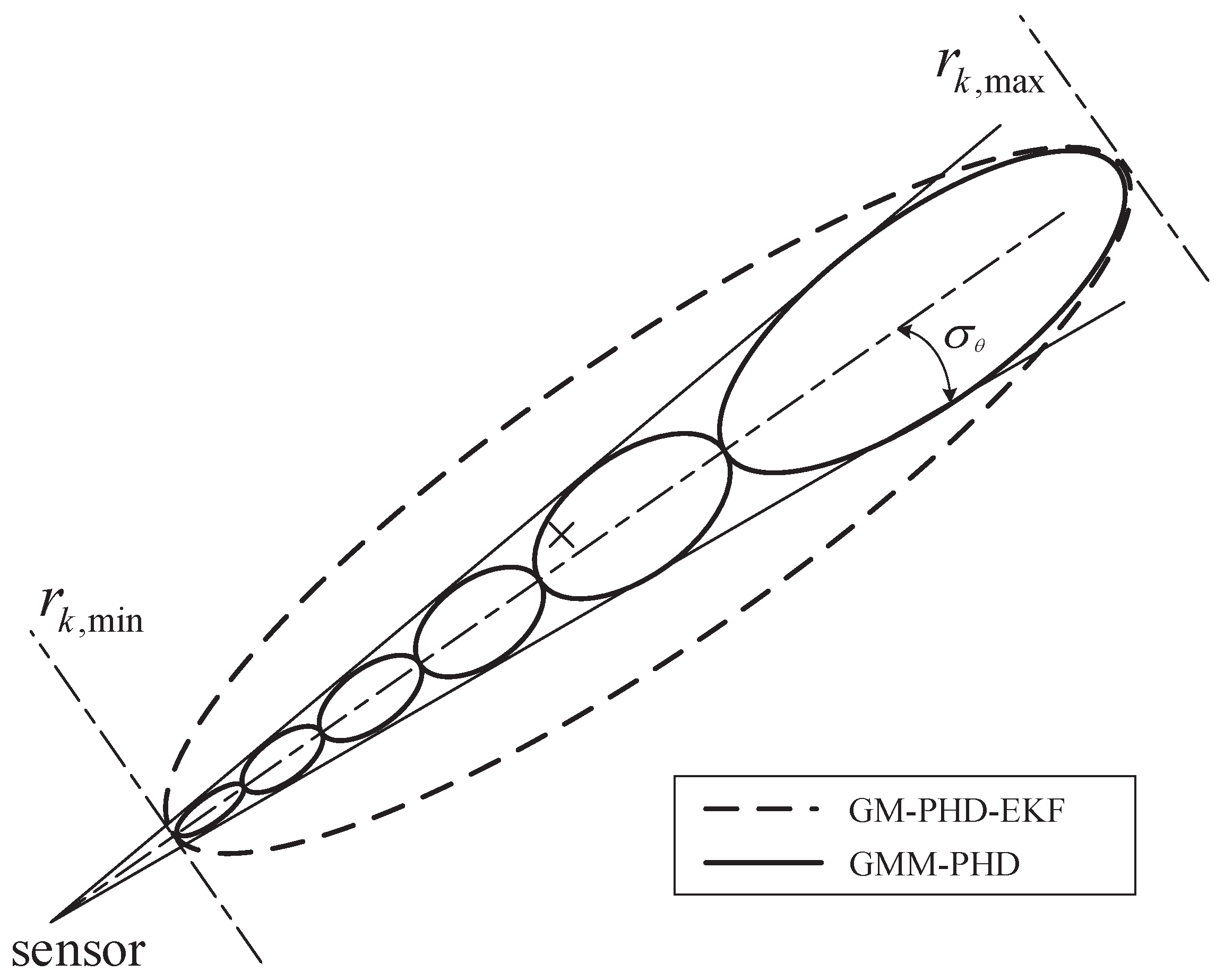
3.2. GMM Likelihood Approximation
3.3. Intensity Update
3.4. Component Management and State Extraction
4. Simulation Experiments
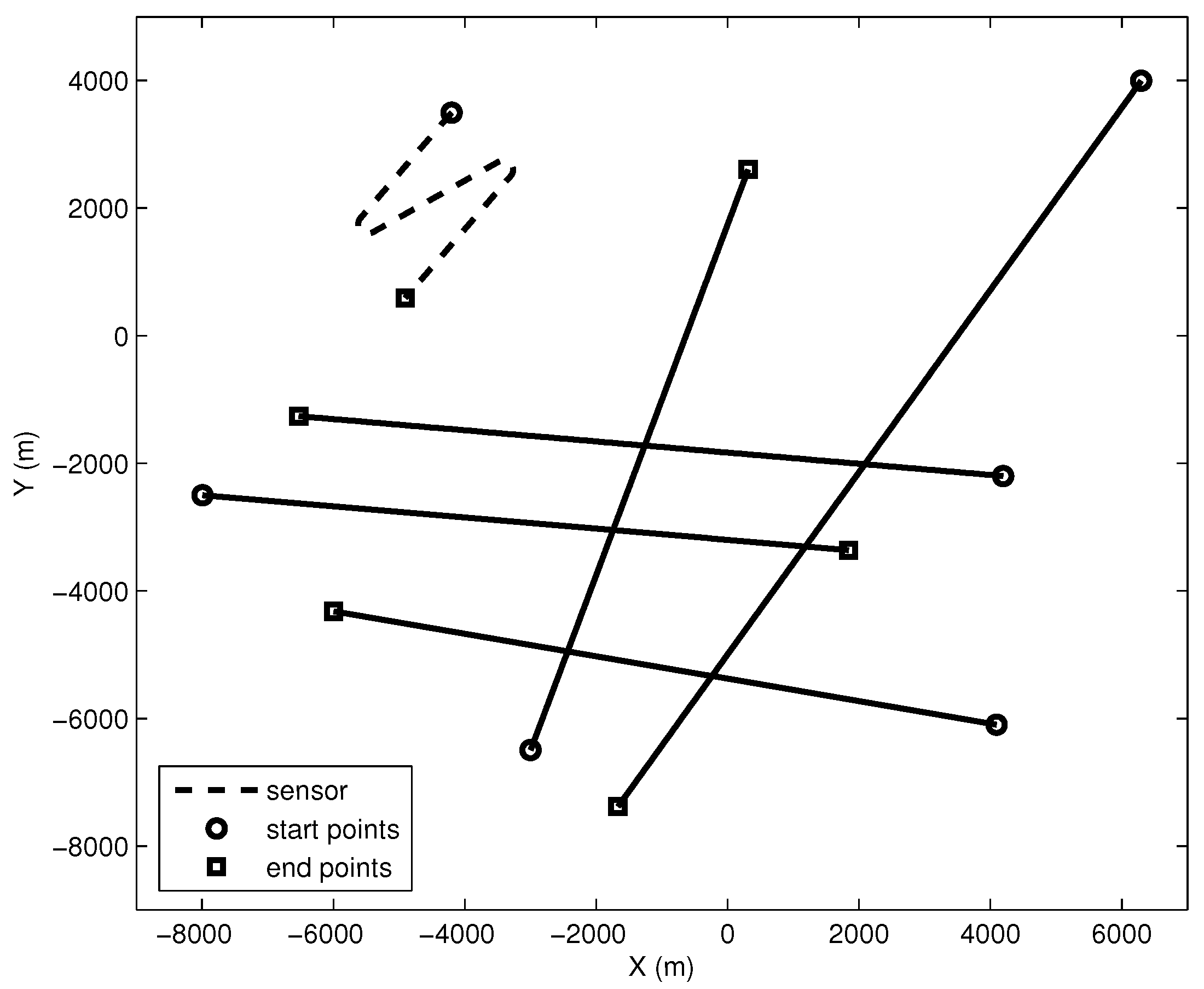
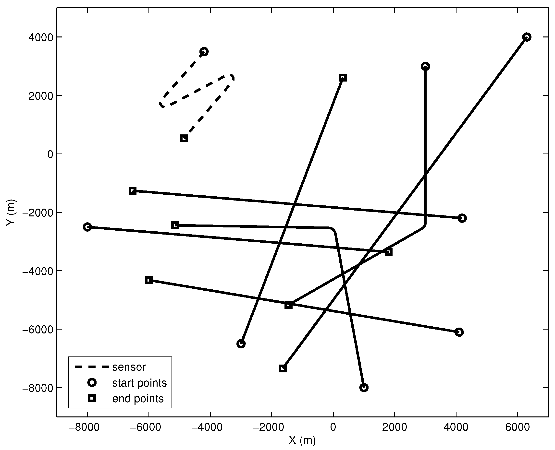
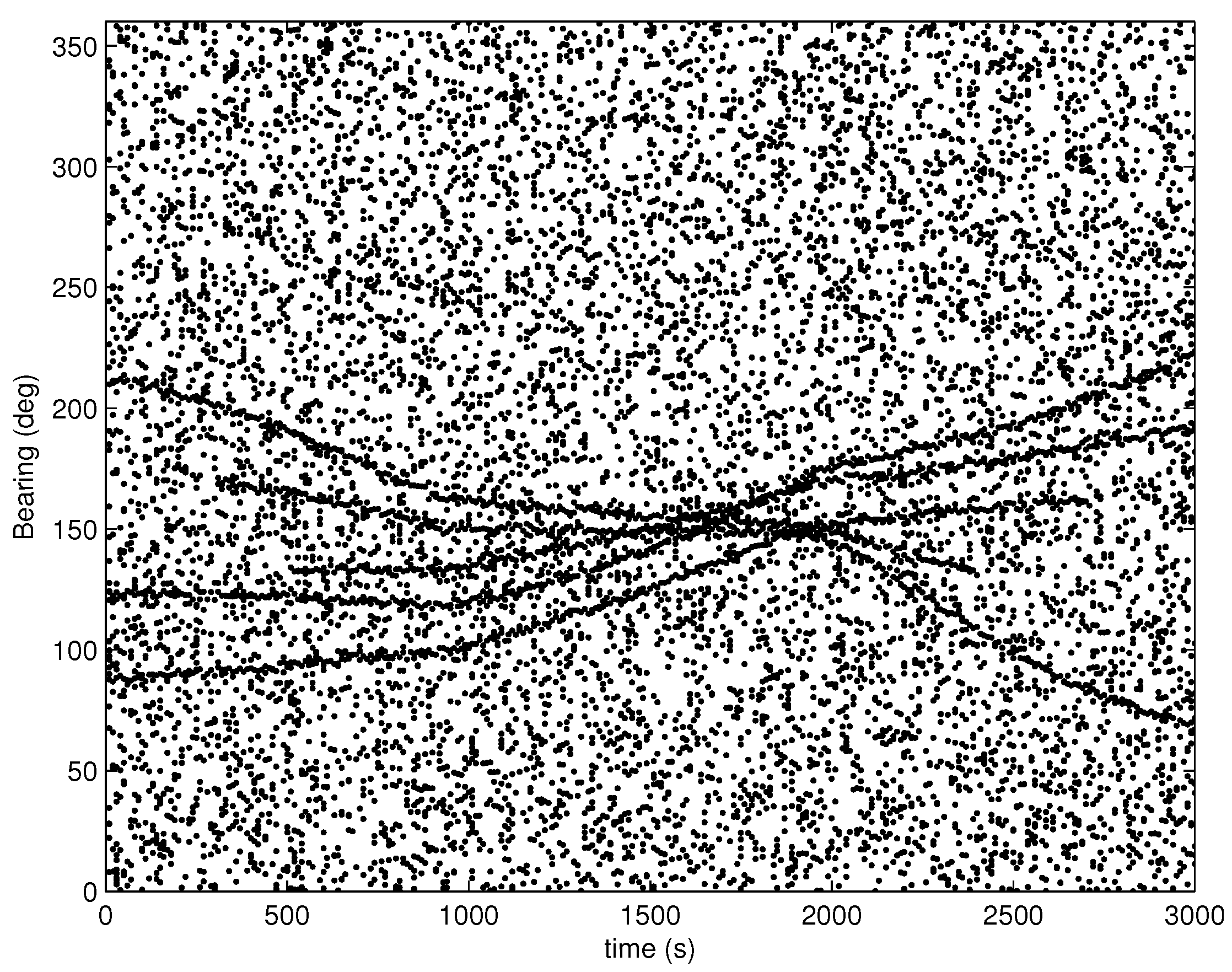
4.1. Simulation Scenarios
4.1.1. Case 1
4.1.2. Case 2
4.1.3. Case 3
4.1.4. Case 4
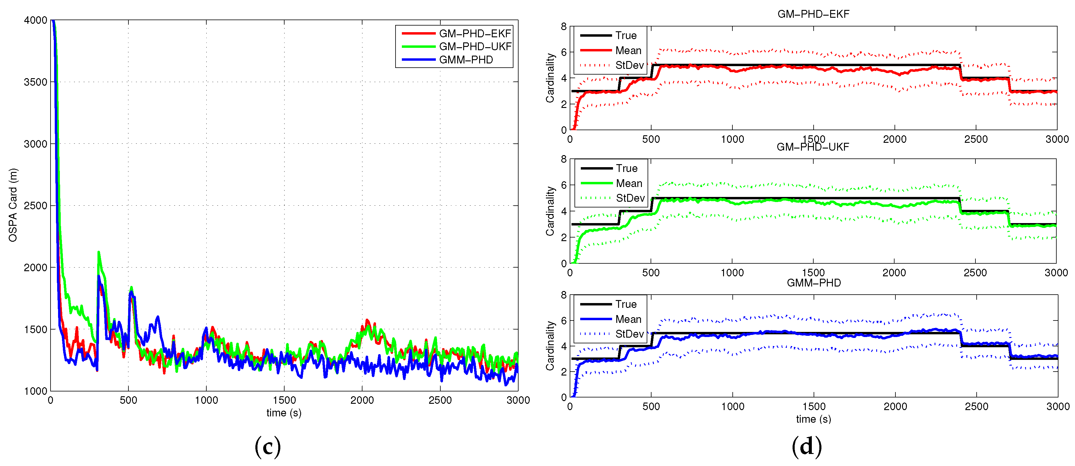
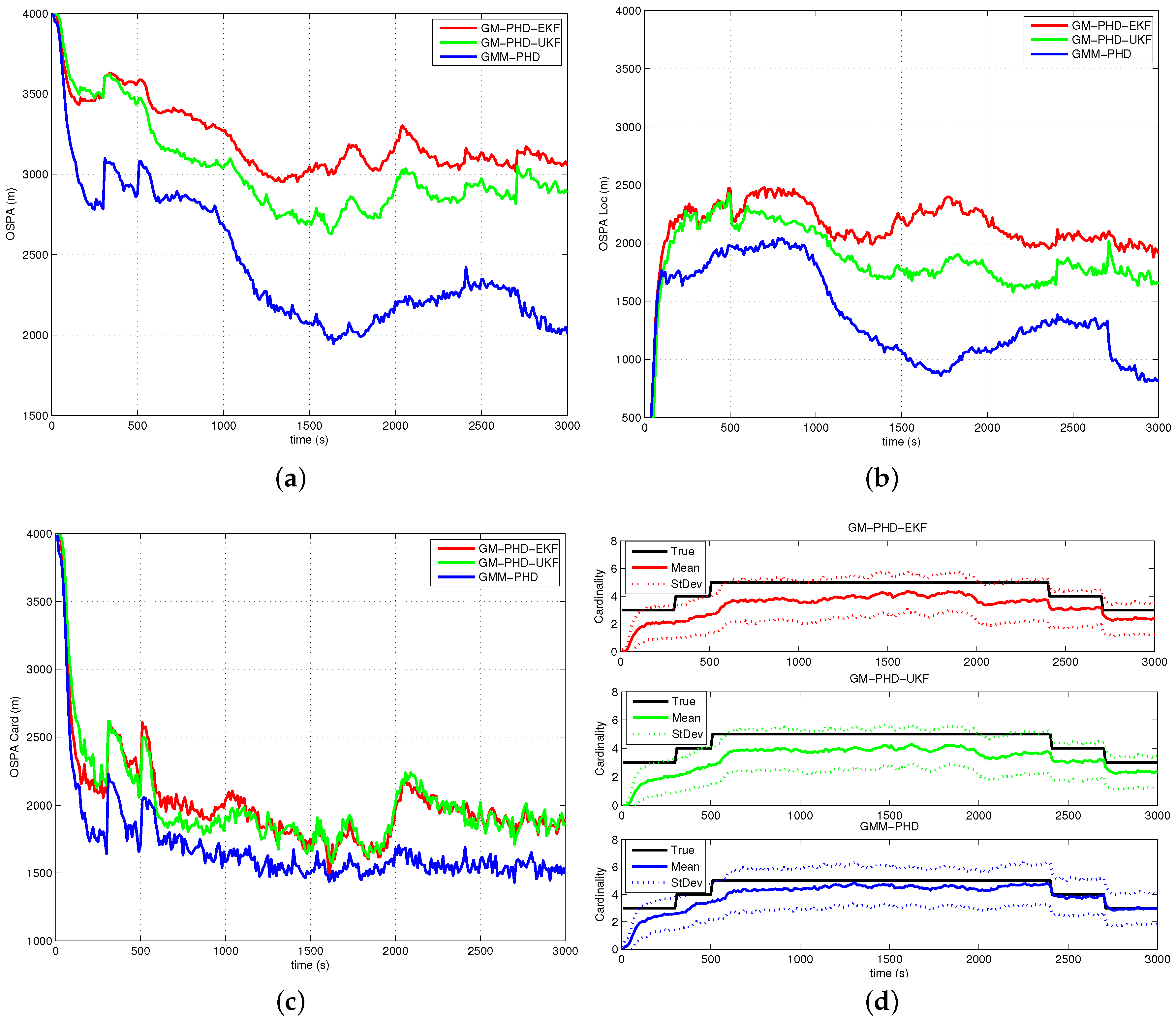
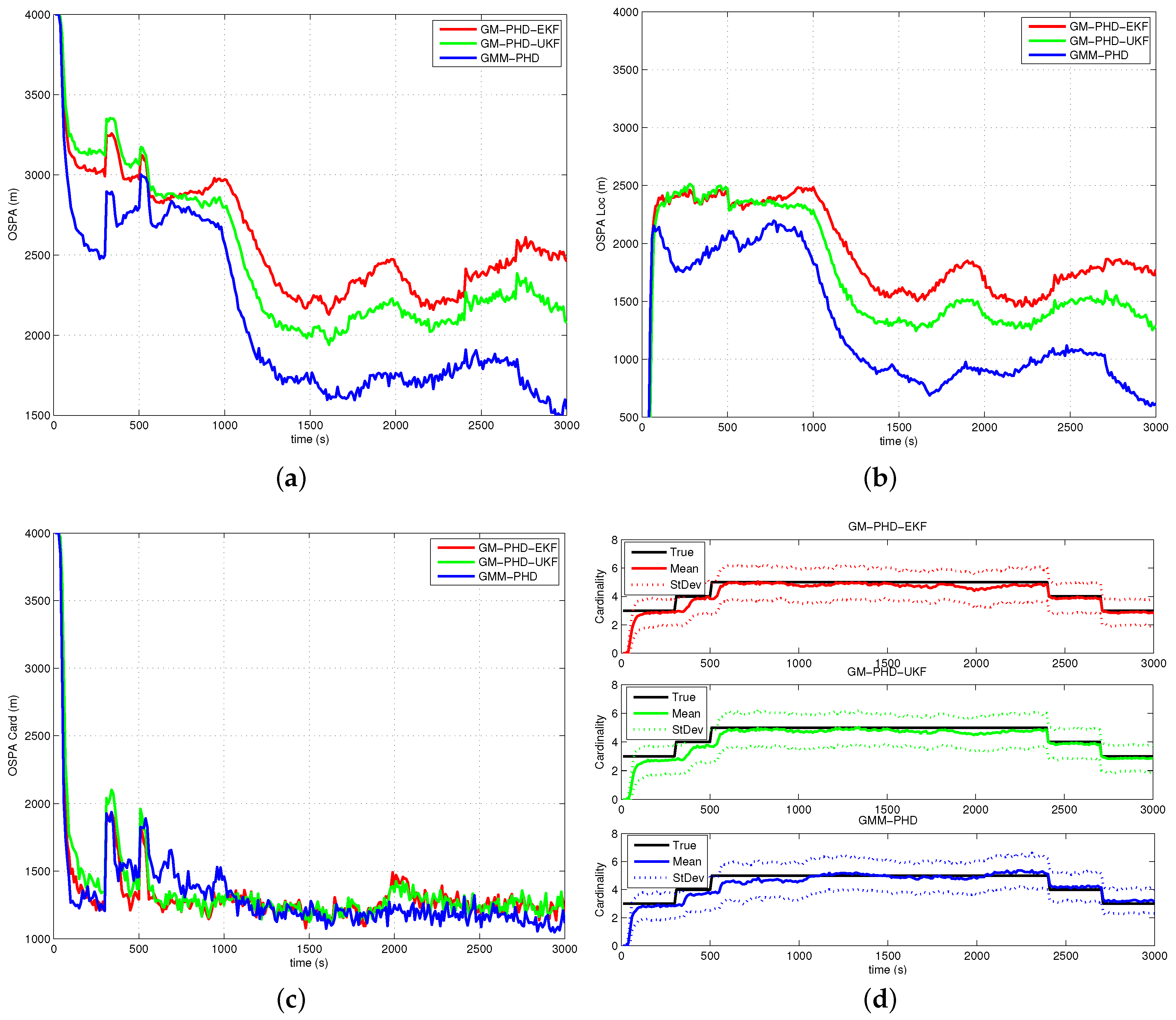
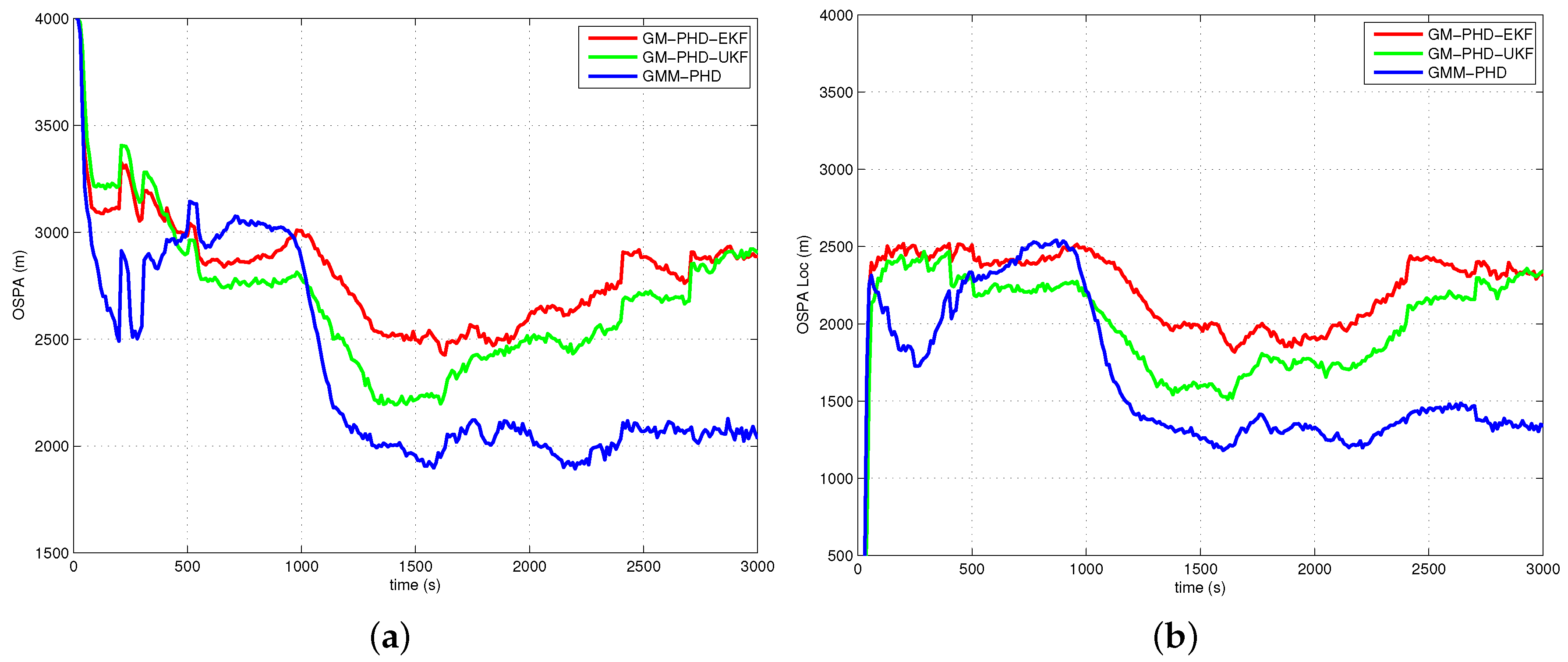
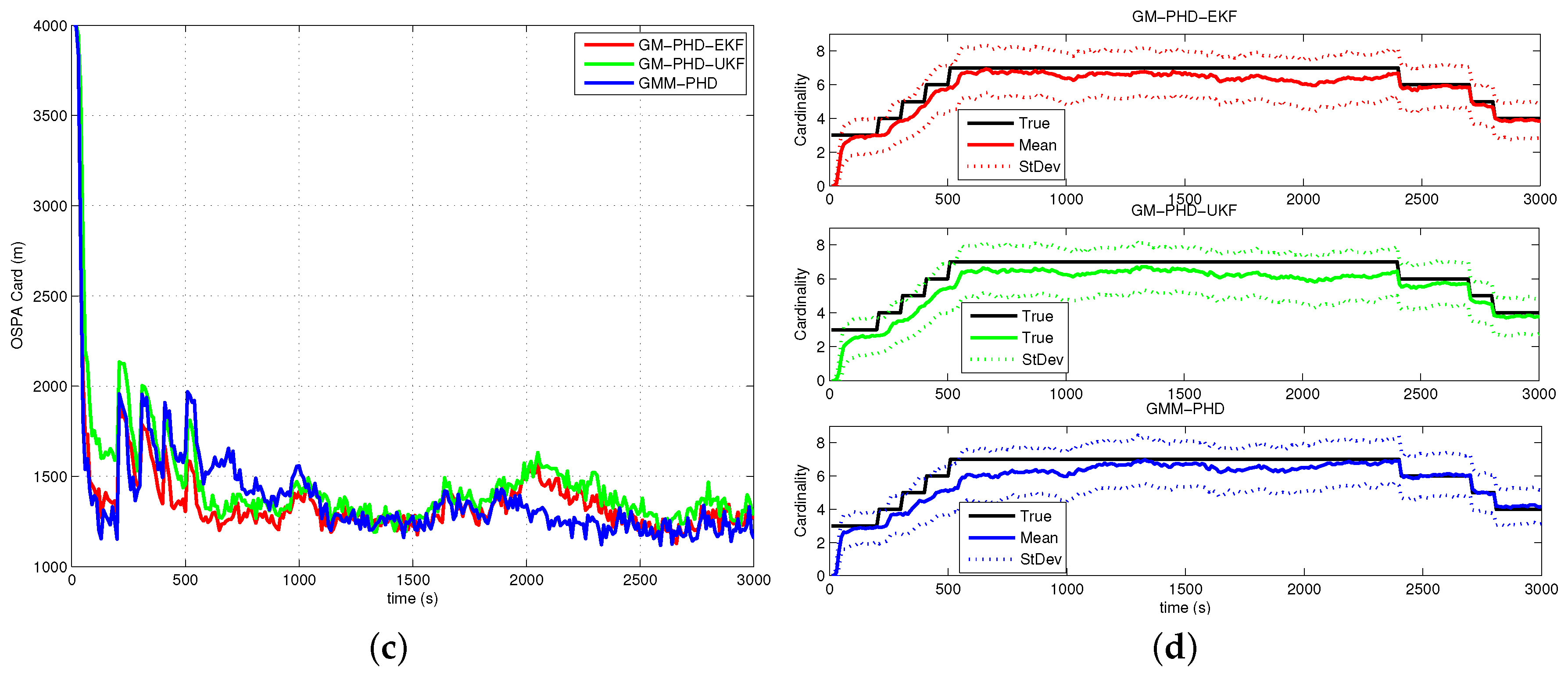
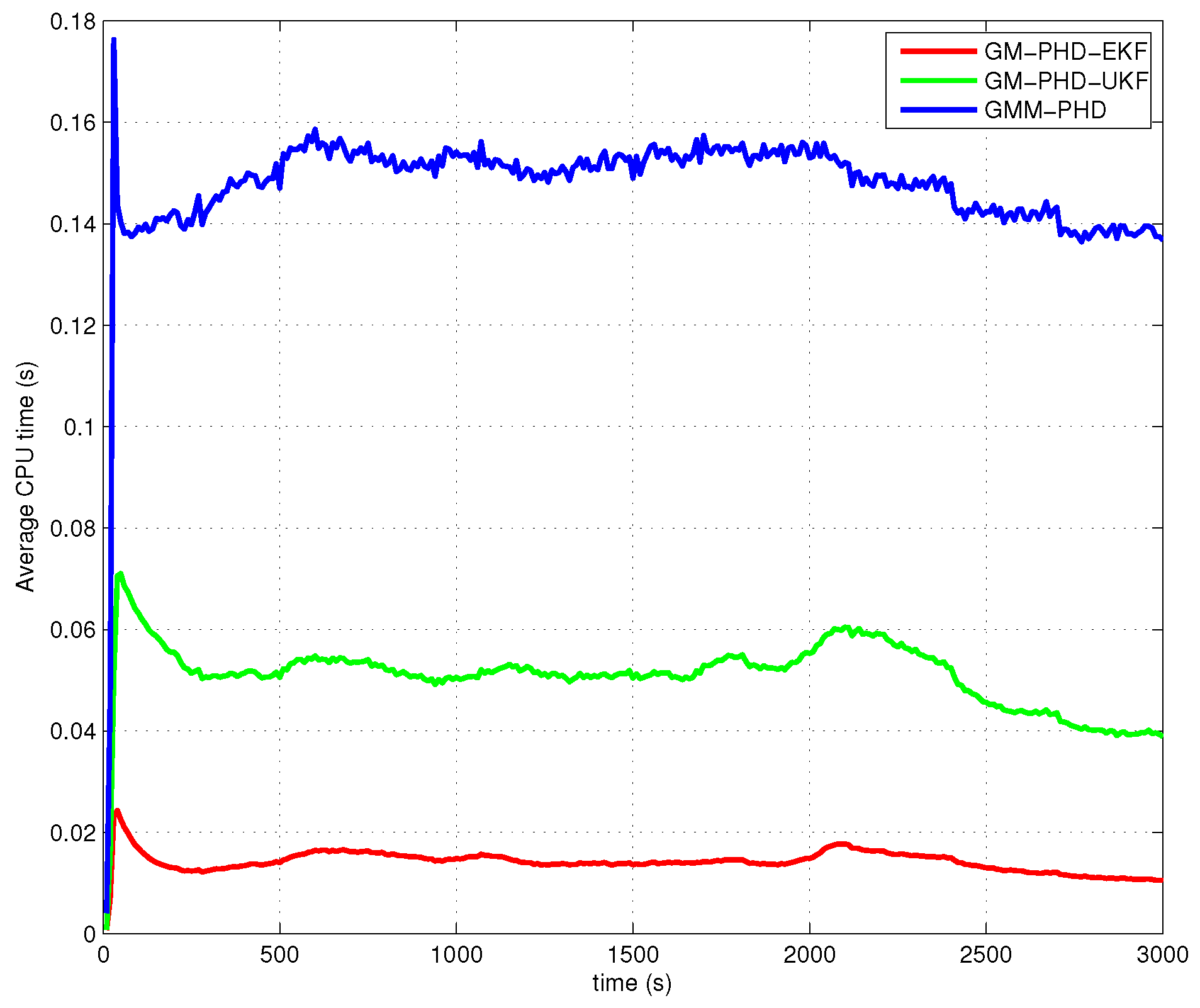
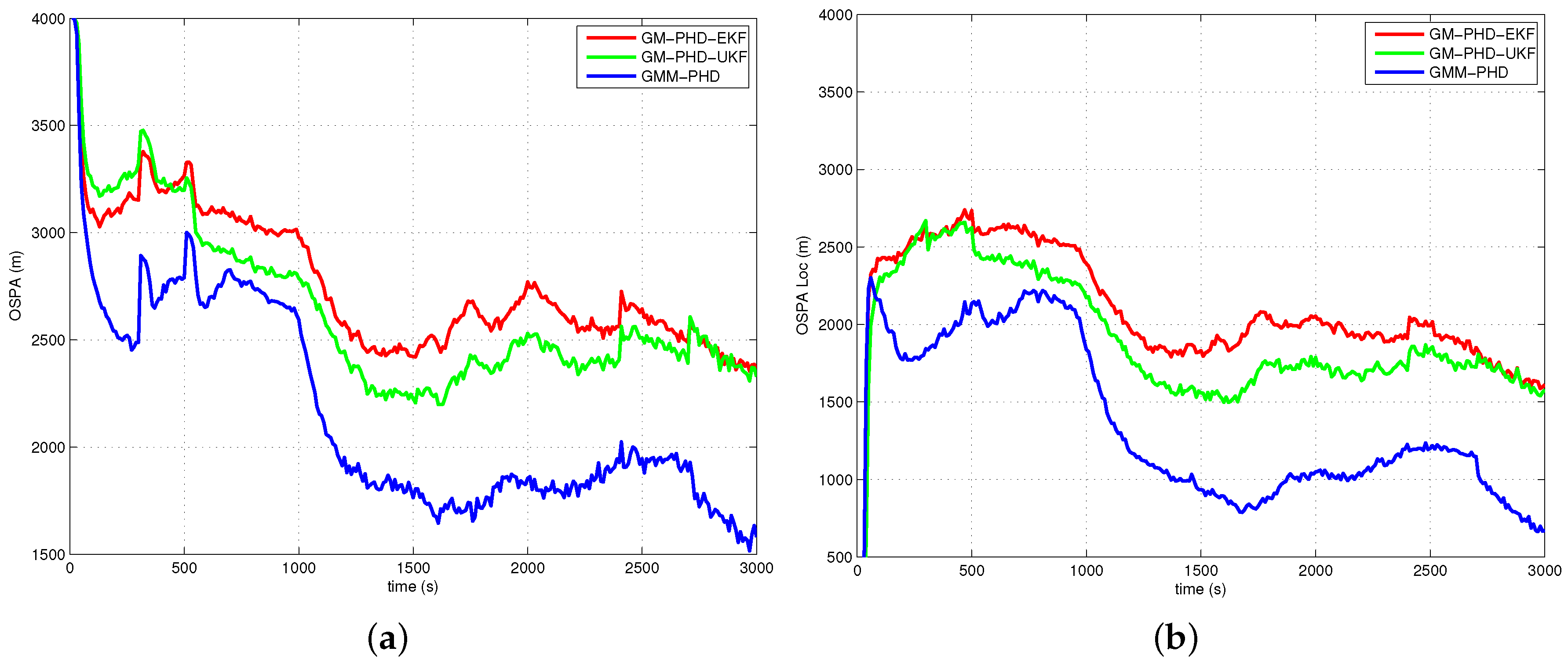
4.2. Simulation Results and Analyses
5. Conclusions
Acknowledgments
Author Contributions
Conflicts of Interest
References
- Bar-Shalom, Y.; Willett, P.K.; Tian, X. Tracking and Data Fusion: A Handbook of Algorithms; YBS Publishing: Storrs, CT, USA, 2011. [Google Scholar]
- Blackman, S.; Popoli, R. Design and Analysis of Modern Tracking Systems; Artech House: Norwood, MA, USA, 1999. [Google Scholar]
- Challa, S.; Morelande, M.; Mušicki, D. Fundamentals of Object Tracking; Cambridge University Press: Cambridge, UK, 2011. [Google Scholar]
- Ristic, B.; Arulampalam, S.; Gordon, N. Beyond the Kalman Filter; Artech House: Norwood, MA, USA, 2004. [Google Scholar]
- Nardone, S.C.; Aidala, V.J. Observability criteria for bearings-only target motion analysis. IEEE Trans. Aerosp. Electron. Syst. 1981, 17, 162–166. [Google Scholar] [CrossRef]
- Tichavsky, P.; Muravchik, C.H.; Nehorai, A. Posterior Cramer-Rao Bounds for discrete-time nonlinear filtering. IEEE Trans. Signal Process. 1998, 46, 1386–1396. [Google Scholar] [CrossRef]
- Arulampalam, S.; Clark, M.; Vinter, R. Performance of the Shifted Rayleigh filter in single-sensor bearings-only tracking. In Proceedings of the 10th International Conference on Information Fusion, Quebec, QC, Canada, 9–12 July 2007; pp. 1–6.
- Beard, M.; Vo, B.T.; Vo, B.N.; Arulampalam, S. A partially uniform target birth model for Gaussian mixture PHD/CPHD filtering. IEEE Trans. Aerosp. Electron. Syst. 2013, 49, 2835–2844. [Google Scholar] [CrossRef]
- Nardone, S.C.; Lindgren, A.G.; Gong, K.F. Fundamental properties and performance of conventional bearings-only target motion analysis. IEEE Trans. Autom. Control 1984, 29, 775–787. [Google Scholar] [CrossRef]
- Kamen, E.W. Multiple target tracking based on symmetric measurement equations. IEEE Trans. Autom. Control 1992, 37, 371–374. [Google Scholar] [CrossRef]
- Mahler, R. Statistical Multisource-Multitarget Information Fusion; Artech House: Norwood, MA, USA, 2007. [Google Scholar]
- Bar-Shalom, Y.; Li, X.R.; Kirubarajan, T. Estimation with Applications to Tracking and Navigation; Wiley: New York, NY, USA, 2001. [Google Scholar]
- Wan, E.A.; van der Merwe, R. The Unscented Kalman filter for nonlinear estimation. In Proceedings of the IEEE Svrnposiurii 2000 (AS-SPCC), Lake Louise, AB, Canada, 4 October 2000.
- Arulampalam, M.S.; Maskell, S.; Gordon, N.; Clapp, T. A tutorial on particle filters for online nonlinear/non-Gaussian Bayesian tracking. IEEE Trans. Signal Process. 2002, 50, 174–188. [Google Scholar] [CrossRef]
- Arasaratnam, I.; Haykin, S. Cubature Kalman filters. IEEE Trans. Autom. Control 1984, 54, 1254–1269. [Google Scholar] [CrossRef]
- Clark, J.M.C.; Vinter, R.B.; Yaqoob, M.M. Shifted Rayleigh filter: A new algorithm for bearings-only tracking. IEEE Trans. Aerosp. Electron. Syst. 2007, 43, 1373–1384. [Google Scholar] [CrossRef]
- Evensen, G. The Ensemble Kalman filter: Theoretical formulation and practical implementation. Ocean Dyn. 2003, 53, 343–367. [Google Scholar] [CrossRef]
- Bar-Shalom, Y.; Li, X.R. Multitarget-Multisensor Tracking: Principles and Techniques; University of Connecticutl: Storrs, CT, USA, 1995. [Google Scholar]
- Reid, D.B. An algorithm for tracking multiple targets. IEEE Trans. Autom. Control 1979, 24, 843–854. [Google Scholar] [CrossRef]
- Li, X.; Li, Y.; Yu, J.; Chen, X.; Dai, M. PMHT Approach for multi-target multi-sensor sonar tracking in clutter. Sensors 2015, 15, 28177–28192. [Google Scholar] [CrossRef] [PubMed]
- Mušicki, D.; Evans, R.J. Joint integrated probabilistic data association: JIPDA. IEEE Trans. Aerosp. Electron. Syst. 2004, 40, 1093–1099. [Google Scholar] [CrossRef]
- Mušicki, D.; Evans, R.J. Multiscan multitarget tracking in clutter with integrated track splitting filter. IEEE Trans. Aerosp. Electron. Syst. 2009, 45, 1432–1447. [Google Scholar] [CrossRef]
- Mušicki, D.; la Scala, B. Multi-target tracking in clutter without measurement assignment. IEEE Trans. Aerosp. Electron. Syst. 2008, 44, 877–896. [Google Scholar] [CrossRef]
- Song, T.L.; Kim, H.W.; Mušicki, D. Iterative joint integrated probabilistic data association for multitarget tracking. IEEE Trans. Aerosp. Electron. Syst. 2015, 51, 642–653. [Google Scholar] [CrossRef]
- Kurien, T. Multitarget Multisensor Tracking; Artech House: Boston, MA, USA, 1990; Volume 1. [Google Scholar]
- Mahler, R. Multitarget bayes filtering via first-order multitarget moments. IEEE Trans. Aerosp. Electron. Syst. 2004, 39, 1152–1178. [Google Scholar] [CrossRef]
- Vo, B.T.; Vo, B.N.; Cantoni, A. Analytic implementations of the cardinalized probability hypothesis density filter. IEEE Trans. Signal Process. 2007, 55, 3553–3567. [Google Scholar] [CrossRef]
- Vo, B.T.; Vo, B.N.; Cantoni, A. The cardinality balanced multi-target multi-bernoulli filter and its implementations. IEEE Trans. Signal Process. 2009, 57, 409–423. [Google Scholar]
- Vo, B.N.; Singh, S.; Doucet, A. Sequential Monte Carlo methods for multitarget filtering with random finite sets. IEEE Trans. Aerosp. Electron. Syst. 2005, 41, 1224–1245. [Google Scholar]
- Liu, Z.; Wang, Z.; Xu, M. Cubature information SMC-PHD for multi-target tracking. Sensors 2016, 16, 653. [Google Scholar] [CrossRef] [PubMed]
- Vo, B.N.; Ma, W.K. The Gaussian mixture probability hypothesis density filter. IEEE Trans. Signal Process. 2006, 54, 4091–4104. [Google Scholar] [CrossRef]
- Beard, M.; Vo, B.T.; Vo, B.N.; Arulampalam, S. Gaussian mixture PHD and CPHD filtering with partially uniform target birth. In Proceedings of the 15th International Conference on Information Fusion, Singapore, 9–12 July 2012; pp. 535–541.
- Schuhmacher, D.; Vo, B.T.; Vo, B.N. A consistent metric for performance evaluation of multi-object filters. IEEE Trans. Signal Process. 2008, 56, 3447–3457. [Google Scholar] [CrossRef]
- Ristic, B.; Clark, D.; Vo, B.N.; Vo, B.T. Adaptive target birth intensity for PHD and CPHD filters. IEEE Trans. Aerosp. Electron. Syst. 2012, 48, 1656–1668. [Google Scholar] [CrossRef]
- Kronhamn, T.R. Bearings-only target motion analysis based on a multihypothesis Kalman filter and adaptive ownship motion control. IEE Proc. Radar Sonar Navig. 1998, 145, 247–252. [Google Scholar] [CrossRef]
- Mušicki, D. Bearings only single-sensor target tracking using Gaussian mixtures. Automatica 2009, 45, 2088–2092. [Google Scholar] [CrossRef]
- Mušicki, D.; Song, T.L.; Kim, W.C.; Nešič, D. Non-linear automatic target tracking in clutter using dynamic Gaussian mixture. IET Radar Sonar Navig. 2012, 6, 937–944. [Google Scholar] [CrossRef]
- Lerro, D.; Bar-Shalom, Y. Tracking with debiased consistent converted measurements versus EKF. IEEE Trans. Aerosp. Electron. Syst. 1993, 29, 1015–1022. [Google Scholar] [CrossRef]
- Beard, M.; Arulampalam, S. Performance of PHD and CPHD filtering versus JIPDA for bearings-only multi-target tracking. In Proceedings of the 15th International Conference on Information Fusion, Singapore, 9–12 July 2012; pp. 542–549.


| Target | Survival Time (s) | Course (degree) | Speed (knots) |
|---|---|---|---|
| #1 | 95 | 8 | |
| #2 | 20 | 7 | |
| #3 | 280 | 8 | |
| #4 | 275 | 7 | |
| #5 | 215 | 10 |
© 2016 by the authors; licensee MDPI, Basel, Switzerland. This article is an open access article distributed under the terms and conditions of the Creative Commons Attribution (CC-BY) license (http://creativecommons.org/licenses/by/4.0/).
Share and Cite
Zhang, Q.; Song, T.L. Improved Bearings-Only Multi-Target Tracking with GM-PHD Filtering. Sensors 2016, 16, 1469. https://doi.org/10.3390/s16091469
Zhang Q, Song TL. Improved Bearings-Only Multi-Target Tracking with GM-PHD Filtering. Sensors. 2016; 16(9):1469. https://doi.org/10.3390/s16091469
Chicago/Turabian StyleZhang, Qian, and Taek Lyul Song. 2016. "Improved Bearings-Only Multi-Target Tracking with GM-PHD Filtering" Sensors 16, no. 9: 1469. https://doi.org/10.3390/s16091469
APA StyleZhang, Q., & Song, T. L. (2016). Improved Bearings-Only Multi-Target Tracking with GM-PHD Filtering. Sensors, 16(9), 1469. https://doi.org/10.3390/s16091469