
A Greedy Scanning Data Collection Strategy for Large-Scale Wireless Sensor Networks with a Mobile Sink


Abstract
:1. Introduction
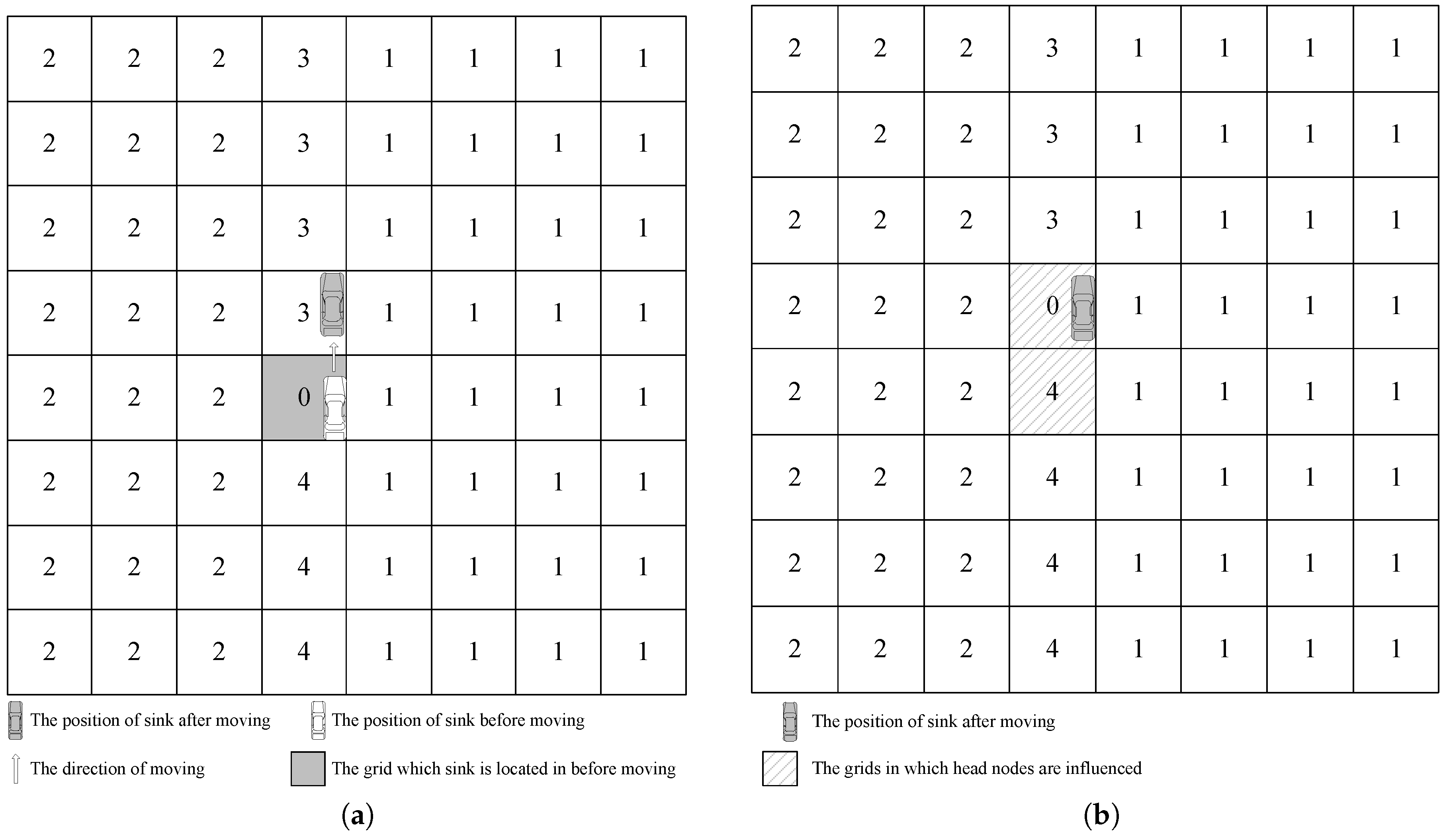
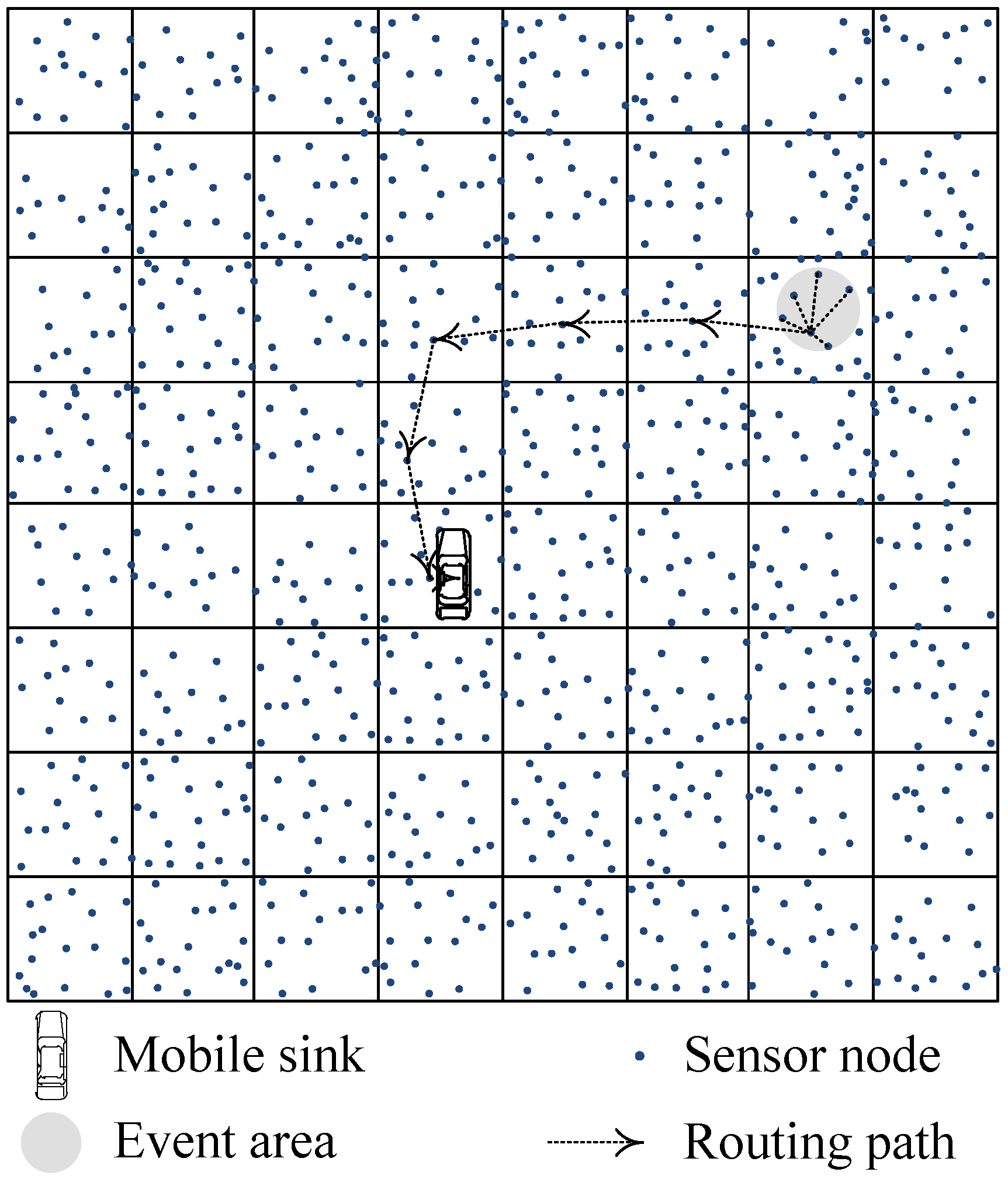
- Sink Location Local Updating Method: In our data collection strategy, the network is divided into virtual grids. When the mobile sink moves from one grid to another, only a few of the grids need to update the location of mobile sink. Sensory data from the whole network can be routed to the sink timely.
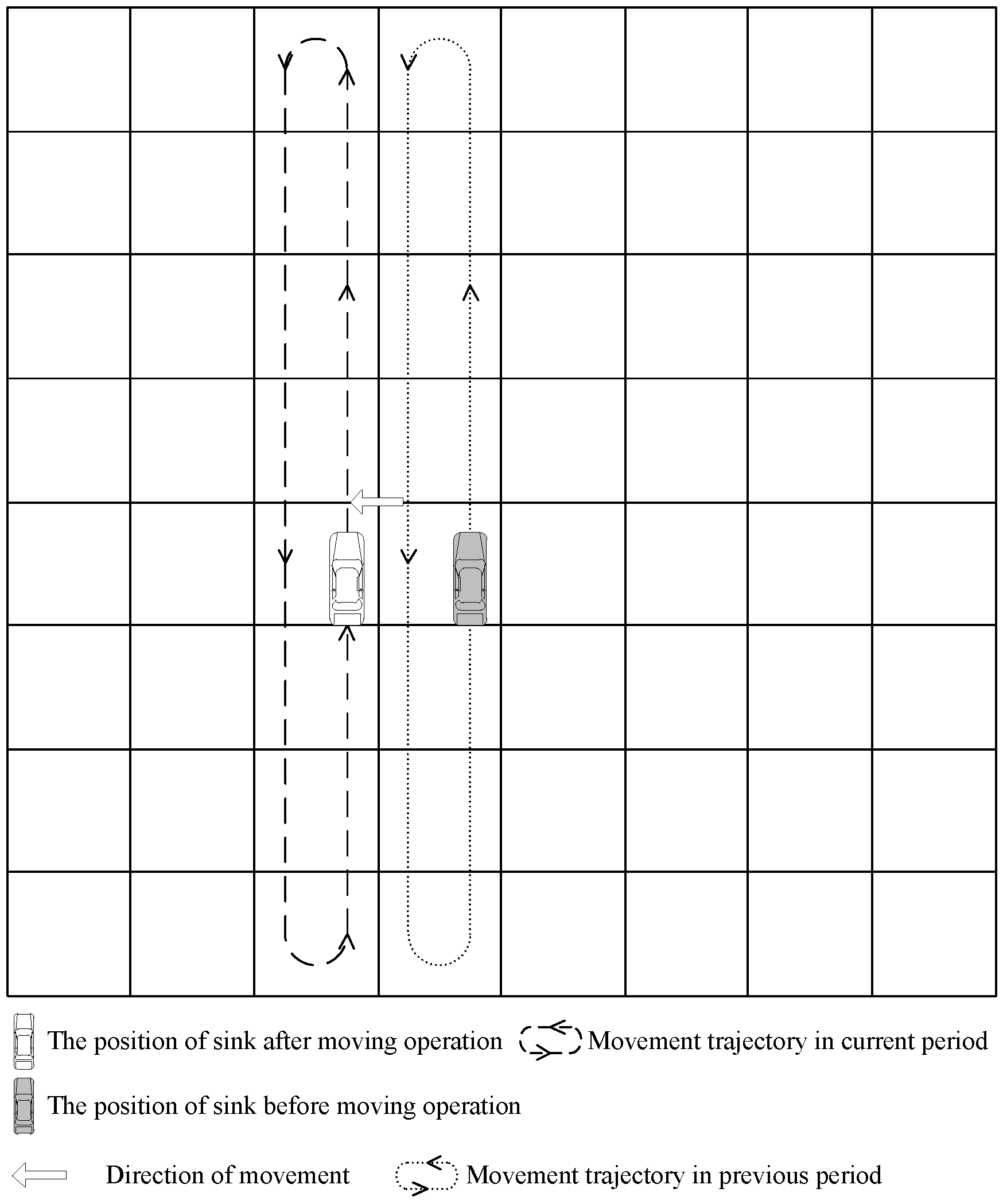
- Greedy Scanning Mobility Pattern: The mobile sink moves like a scanning curve in the screen of radar. According to the sum of data received from each direction, the mobile sink makes the decision to move to the area with more sensory data.
2. Related Works
2.1. Overview
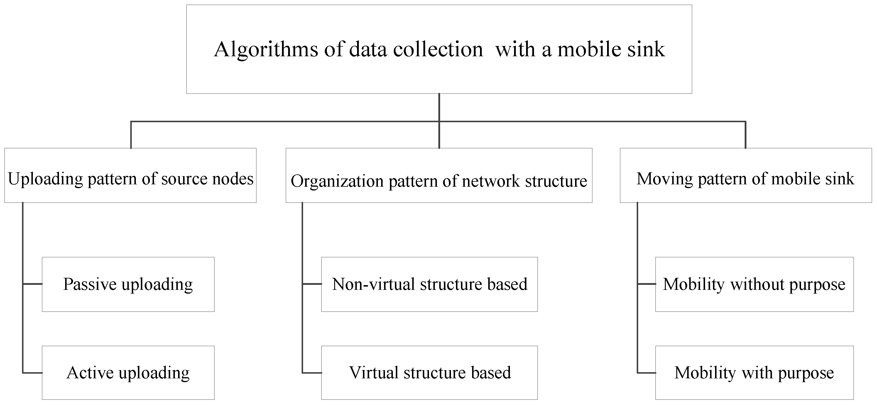
- (1)
- Uploading pattern of source nodes;
- (2)
- Organization pattern of network structure;
- (3)
- Moving pattern of mobile sink.
2.2. Uploading Pattern of Source Nodes
2.2.1. Passive Uploading Pattern
2.2.2. Active Uploading Pattern
2.3. Organization Pattern of Network Structure
2.3.1. Non-Virtual Structure Based Pattern
2.3.2. Virtual Structure Based Pattern
2.4. Moving Pattern of Mobile Sink
2.4.1. Mobility without Purpose Pattern
2.4.2. Mobility with Purpose Pattern
2.5. Summary
3. Greedy Scanning Data Collection Strategy
3.1. Network Model
- Network initialization: To achieve the goal of updating sink location in a local area, the network area is divided into virtual grids. Nodes in the same grid form a group. The initialization process includes the grid structure establishment, head nodes election and neighbor table establishment. The details are discussed in Section 3.2.
- Data collection: In this phase, the way of data routing is proposed first. With the cooperation of virtual grid structure, this data routing way can deliver sensory data to the mobile sink easily. Whereafter, we talk about the moving pattern of the mobile sink with which energy consumption of network can be balanced. To minimize the energy cost in updating sink location information, the local updating with virtual grid structure is discussed at the end of this phase.
- Head nodes re-election: The long time working of head nodes may lead to network energy being unbalanced and lifetime being decreased. To improve the performance of the network, the re-election of head nodes is discussed in Section 3.4.
3.2. Network Initialization
3.2.1. The Establishment of Virtual Grid Structure
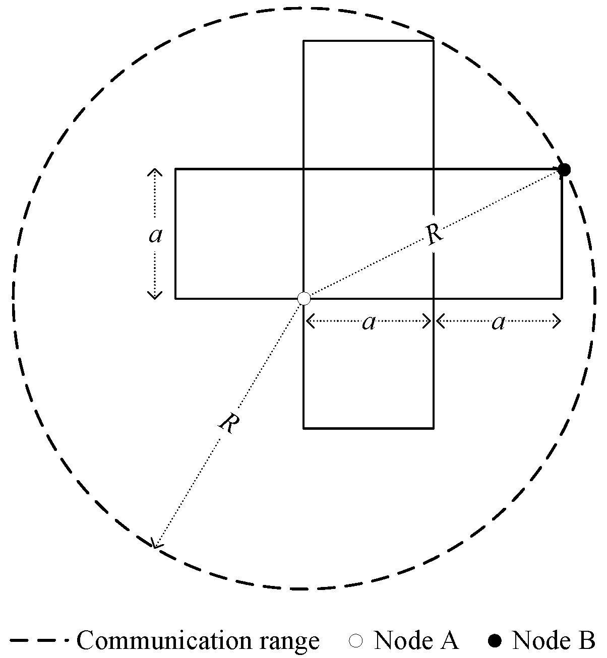
Step 1. Calculate the Virtual Grid Cell Side Length
Step 2. Broadcast the Sink Initial Location and Grid Cell Side Length
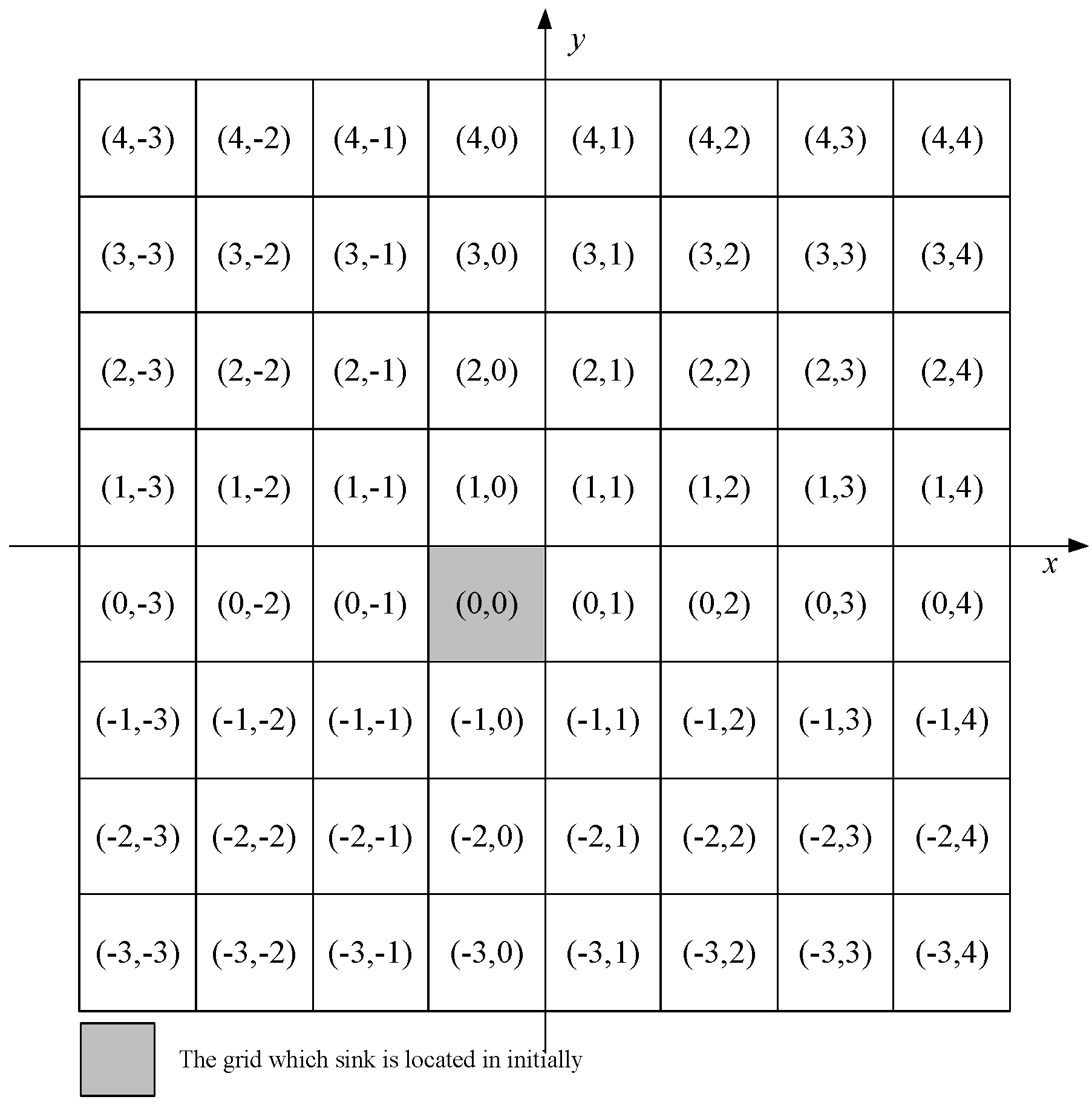
Step 3. Calculate the for Every Grid Cell
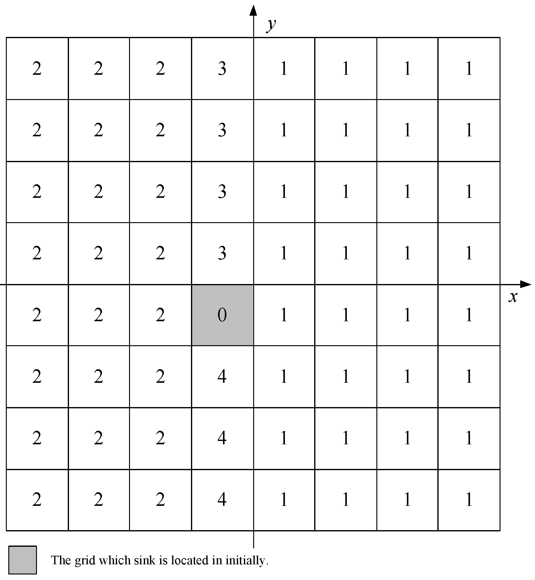
Step 4. Calculate the for Every Grid Cell
- The current grid cell is the ;
- The current grid cell is located in the right side of column that belongs to;
- The current grid cell is located in the left side of column that belongs to;
- The current grid cell is right above ;
- The current grid cell is right under ;
3.2.2. The Election of Head Nodes
3.2.3. The Establishment of Neighbor Table
3.3. Data Collection
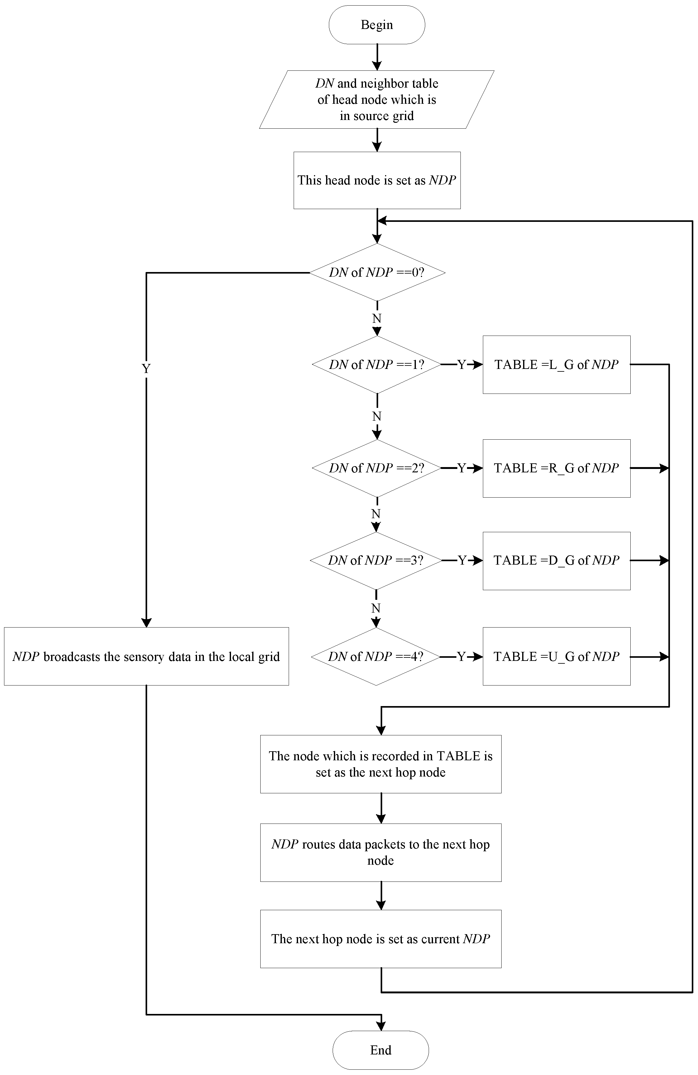
3.3.1. Data Routing
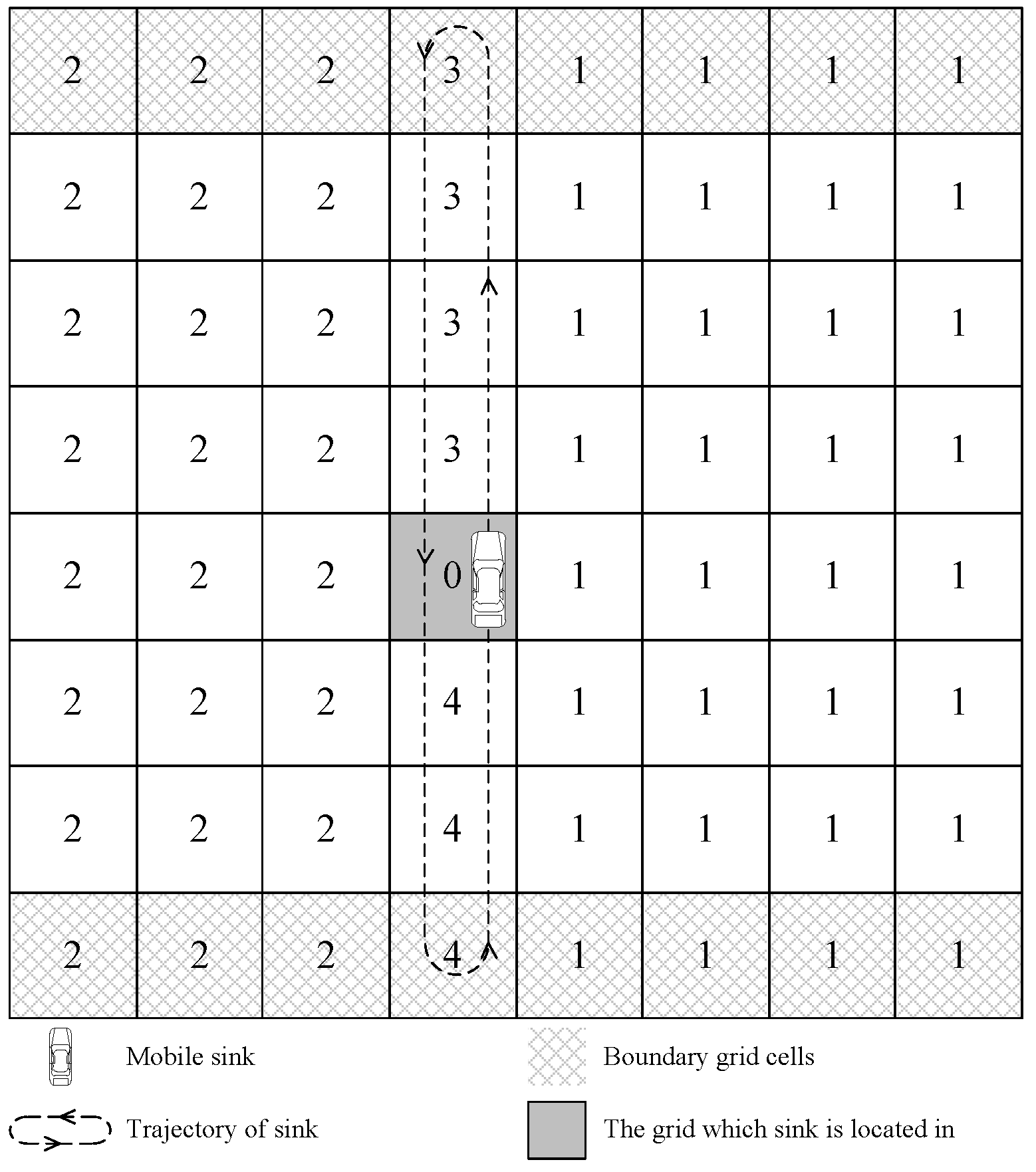
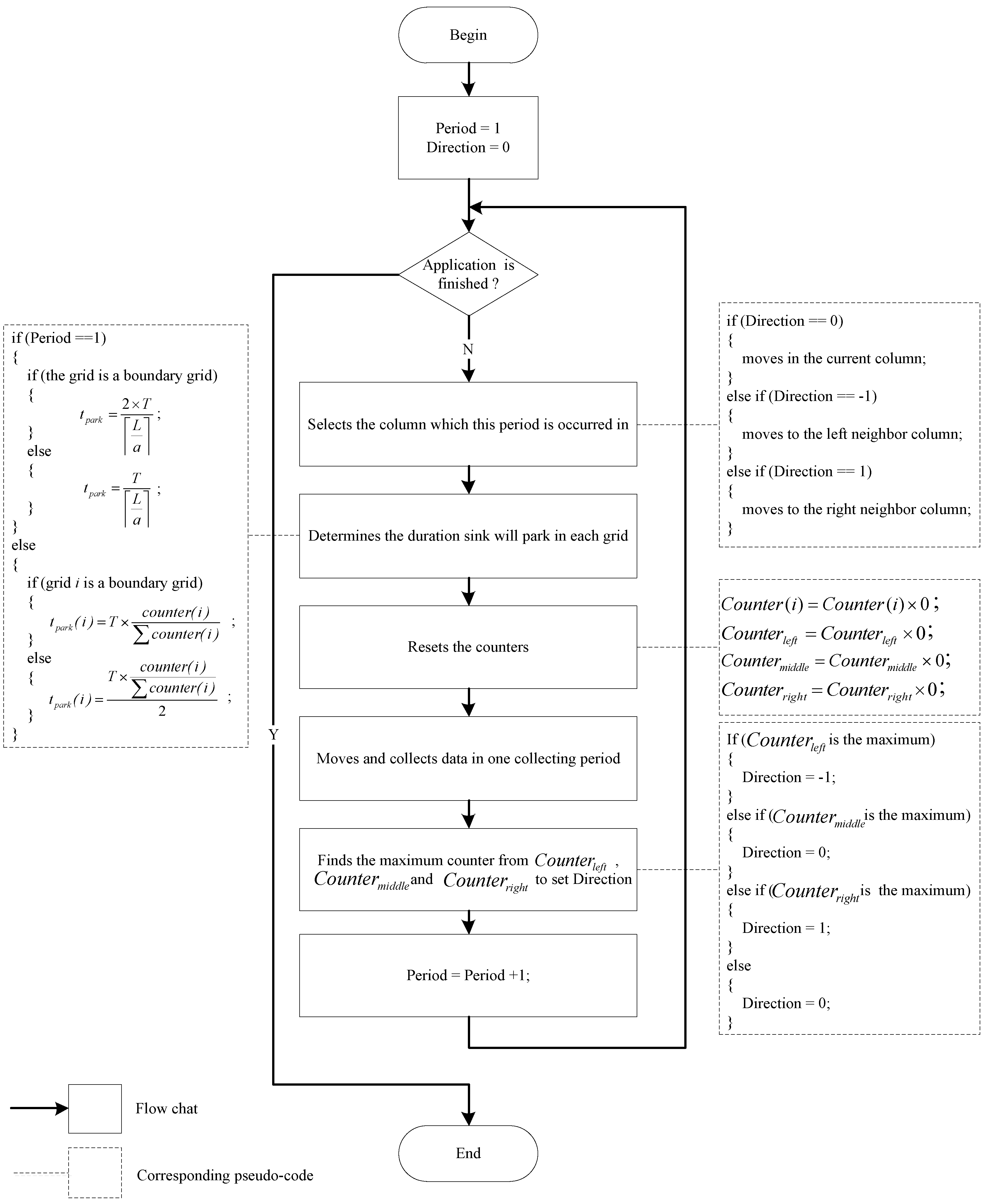
3.3.2. Sink Trajectory Planning
- (1)
- If the grid of row i is a non-boundary grid, then the parking time in this grid is:The total time sink spends in this grid for a single trip is:
- (2)
- If the grid of row i is a boundary grid, then the parking time in this grid is:The total time sink spends in this grid is:
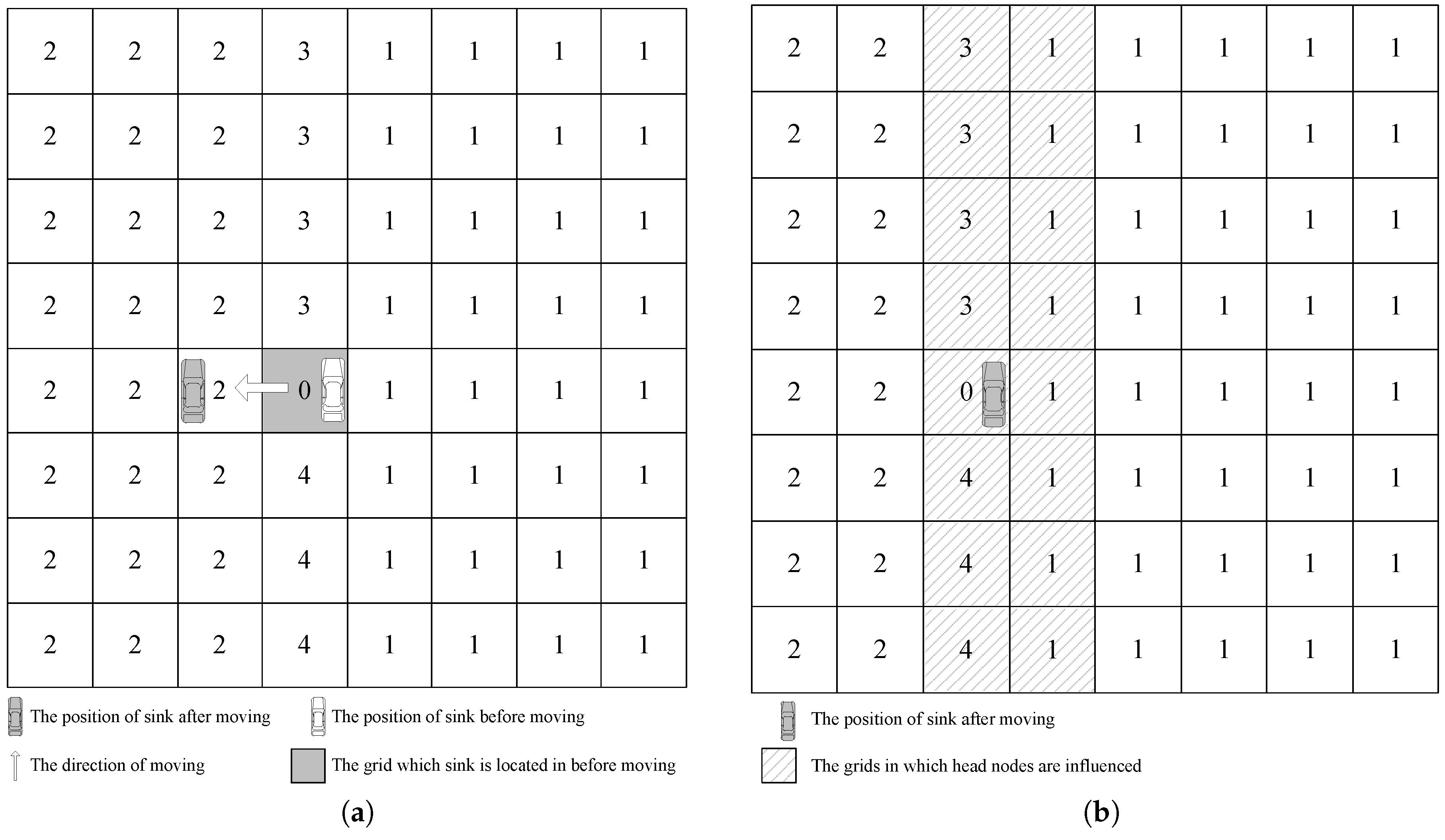
3.3.3. Location Information Local Updating
3.4. Head Nodes Re-Election
4. Simulation and Performance Evaluation
4.1. Simulation Model
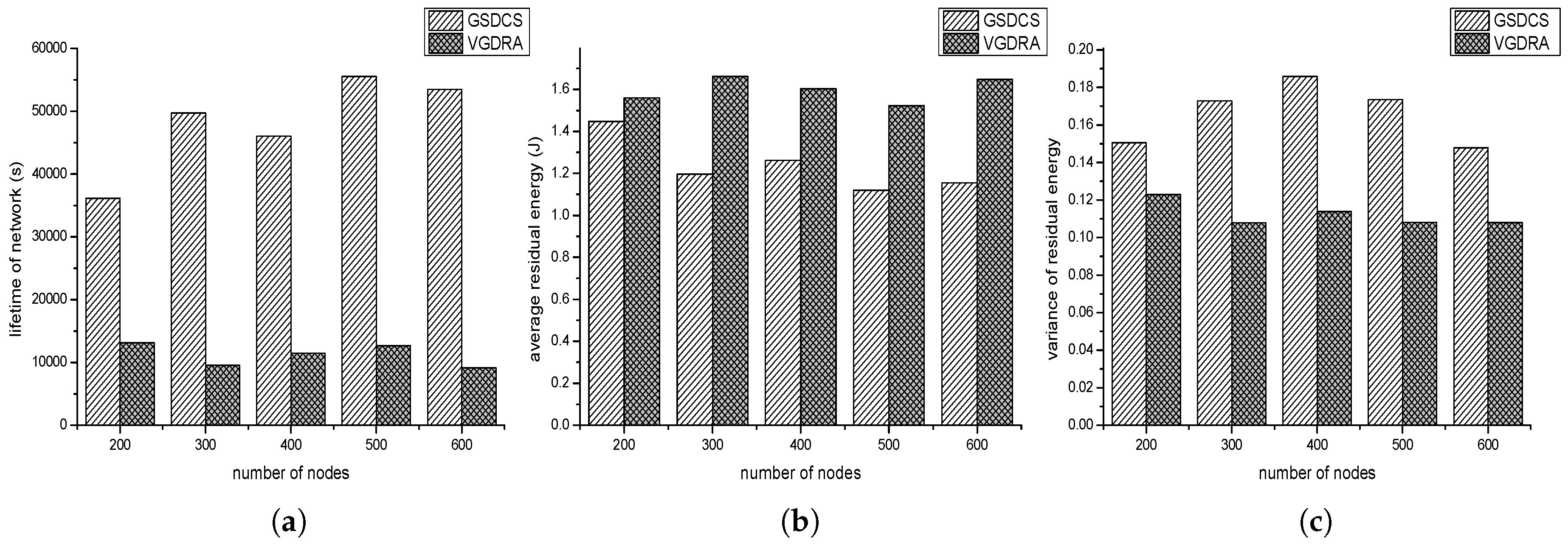
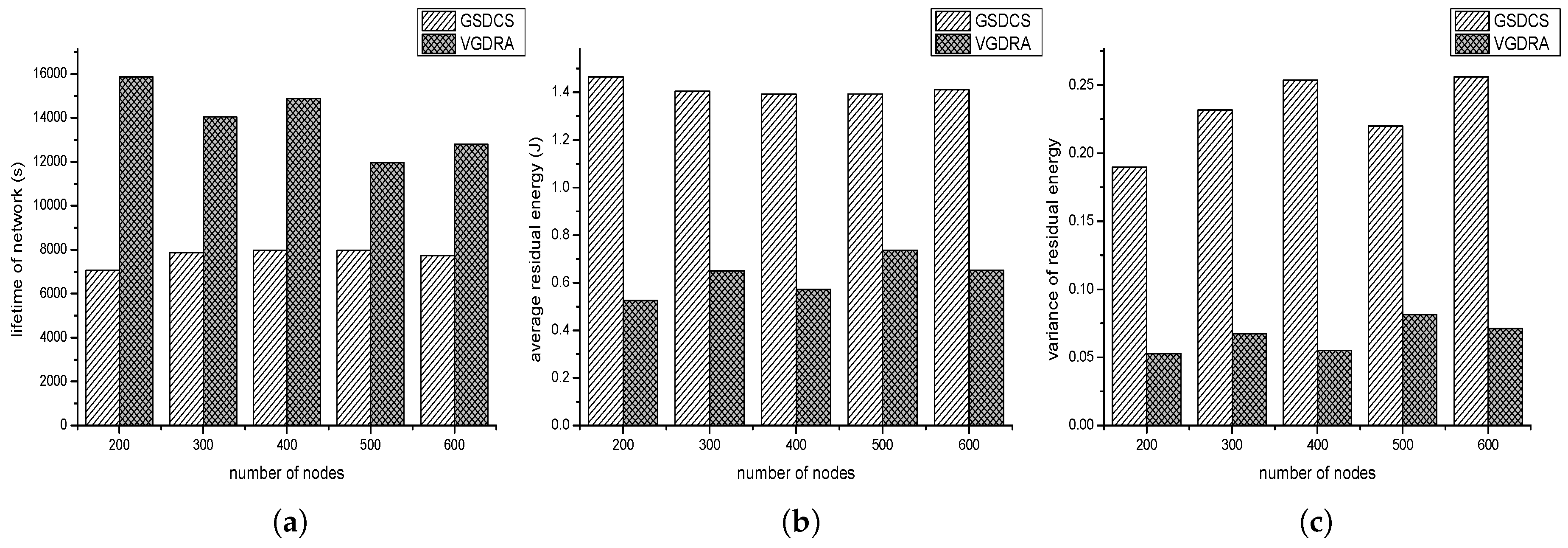
- Lifetime: The time when the first node runs out of its energy.
- Average Residual Energy: The average residual energy of all nodes when the network is ended.
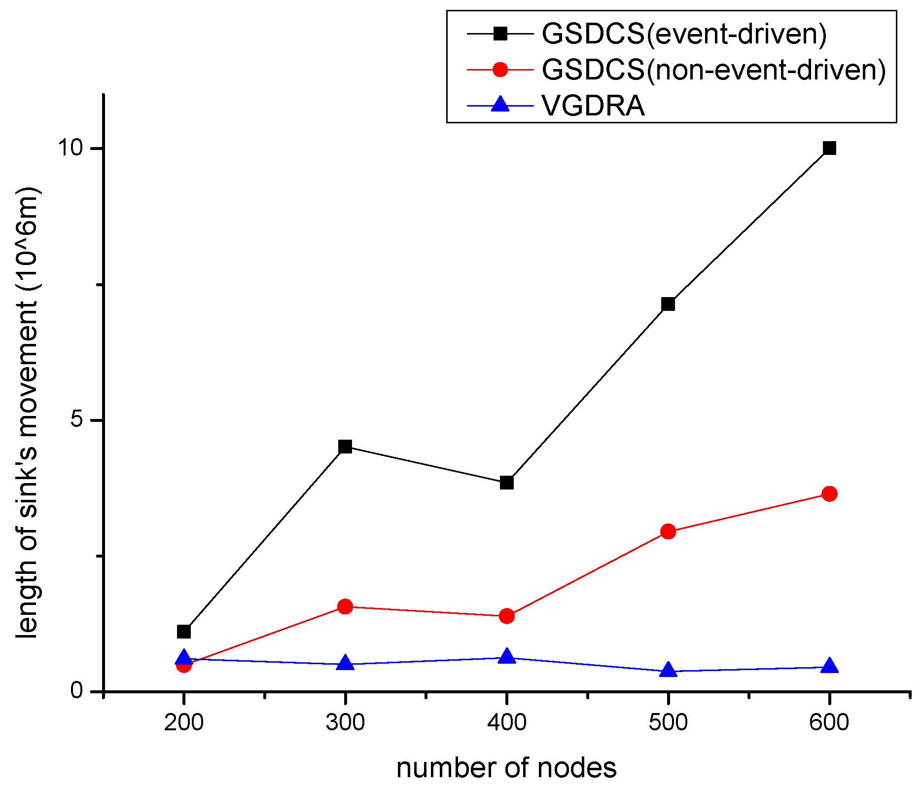
- Length of Sink’s Movement: The length of sink’s trajectory when the network is end.
- Variance of Residual Energy: The variance of all nodes’ residual energy when the network is ended.
- Number of Data Packets Collected: The number of data packets collected by sink when the network is ended.
4.2. Performance Analysis under Different Parameters
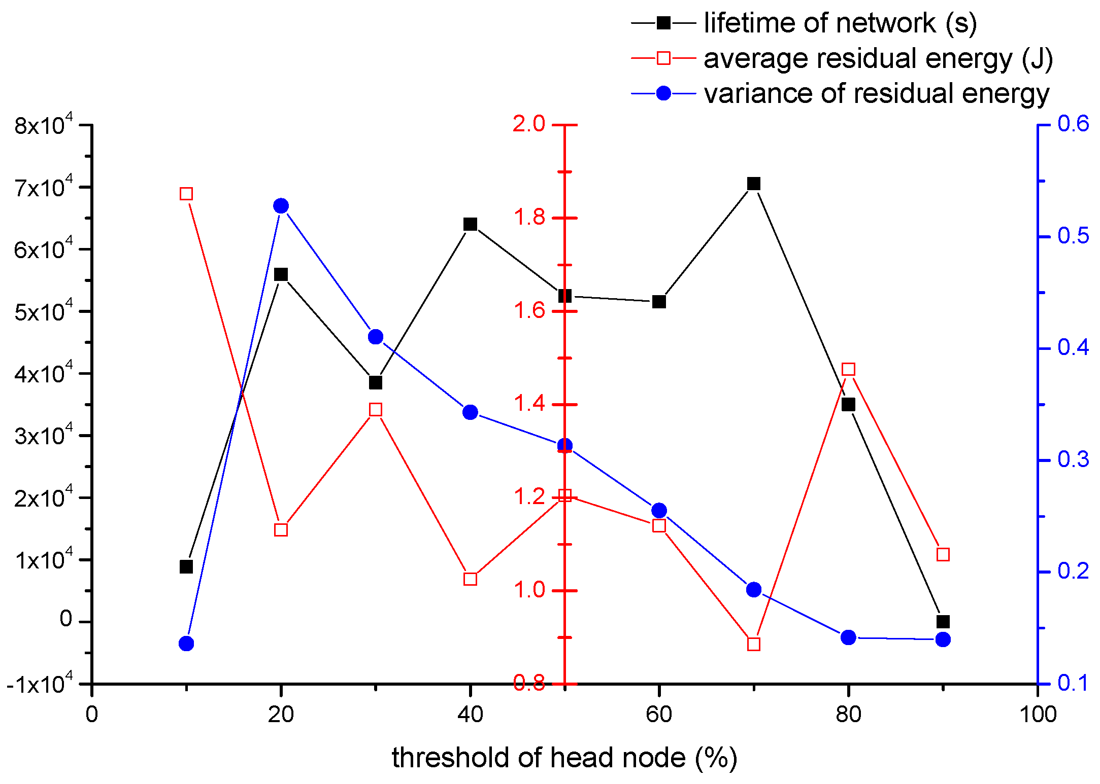
4.2.1. The Impact of Head Nodes’ Threshold
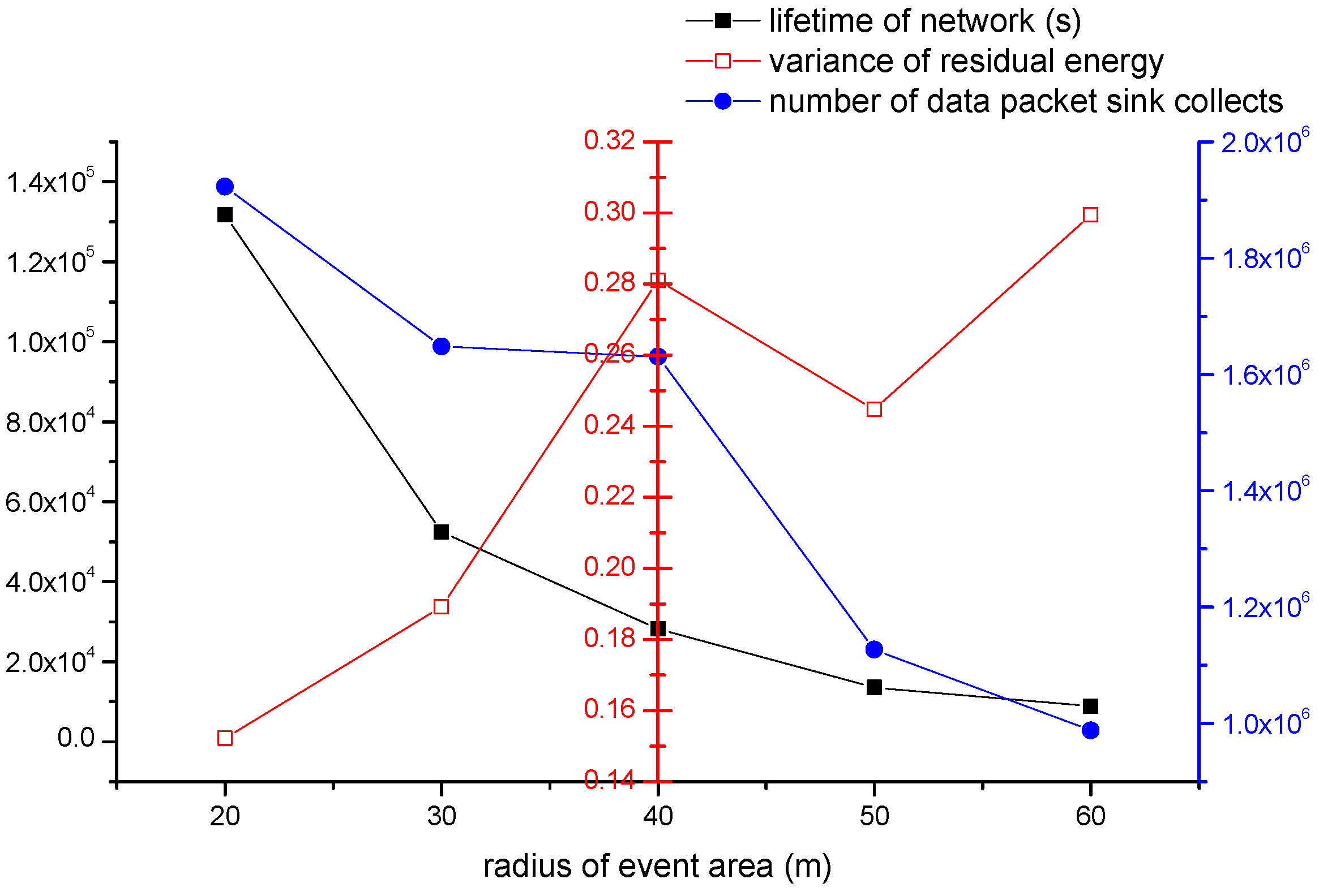
4.2.2. The Impact of Event Area’s Radius
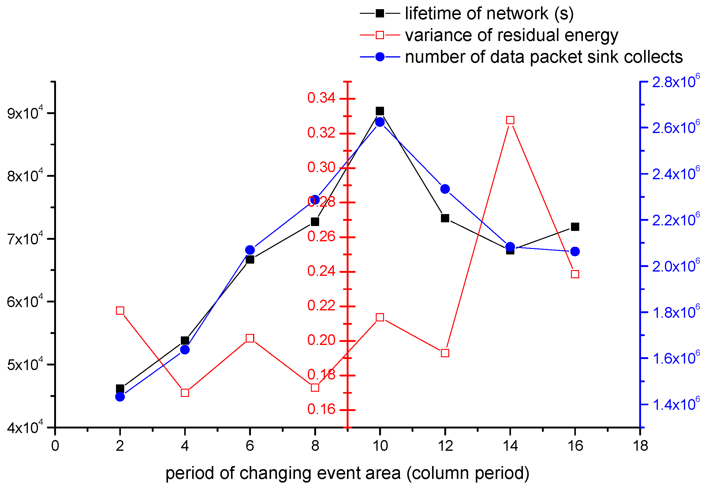
4.2.3. The Impact of Period of Changing Event Area
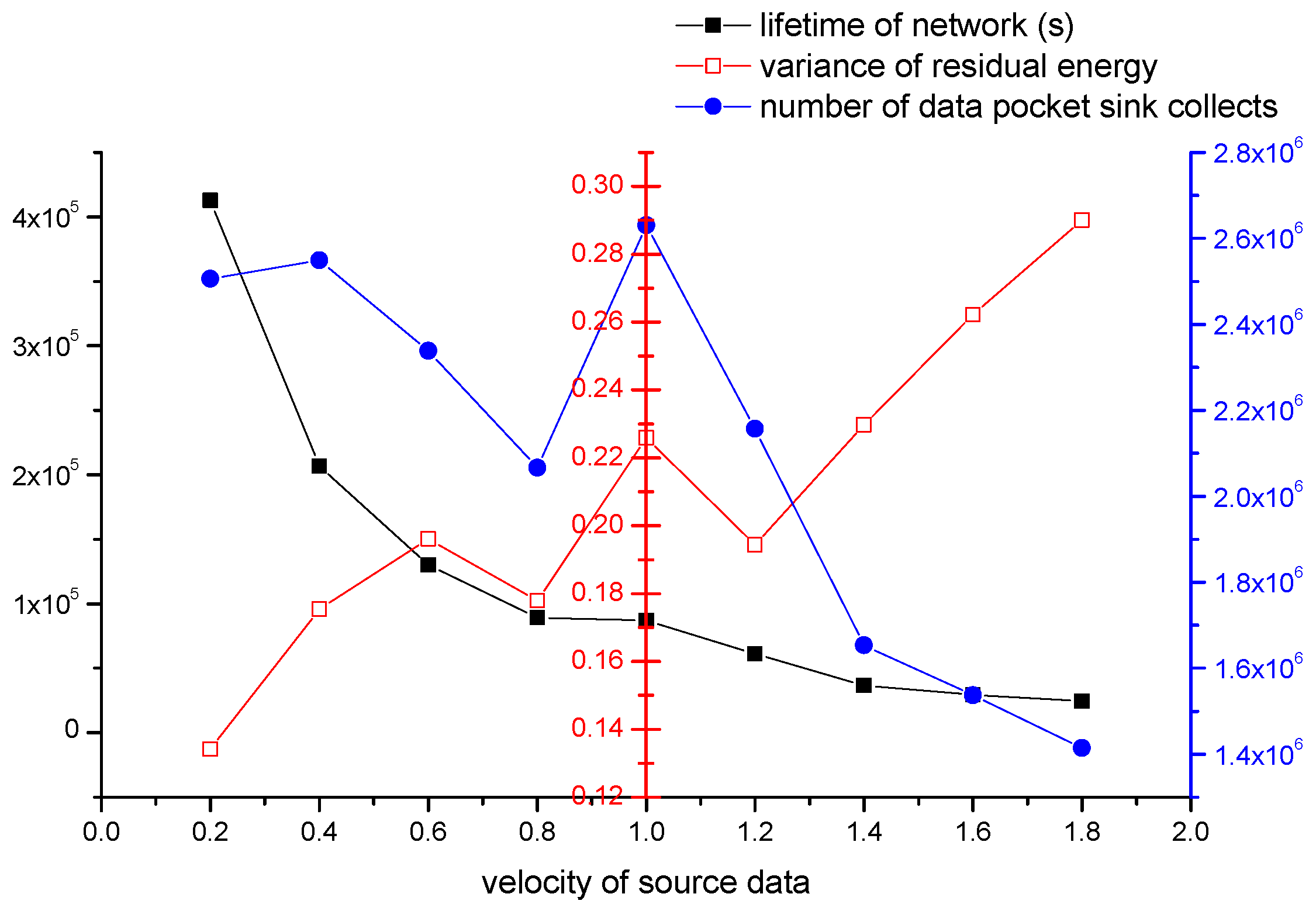
4.2.4. The Impact of Velocity of Source Data
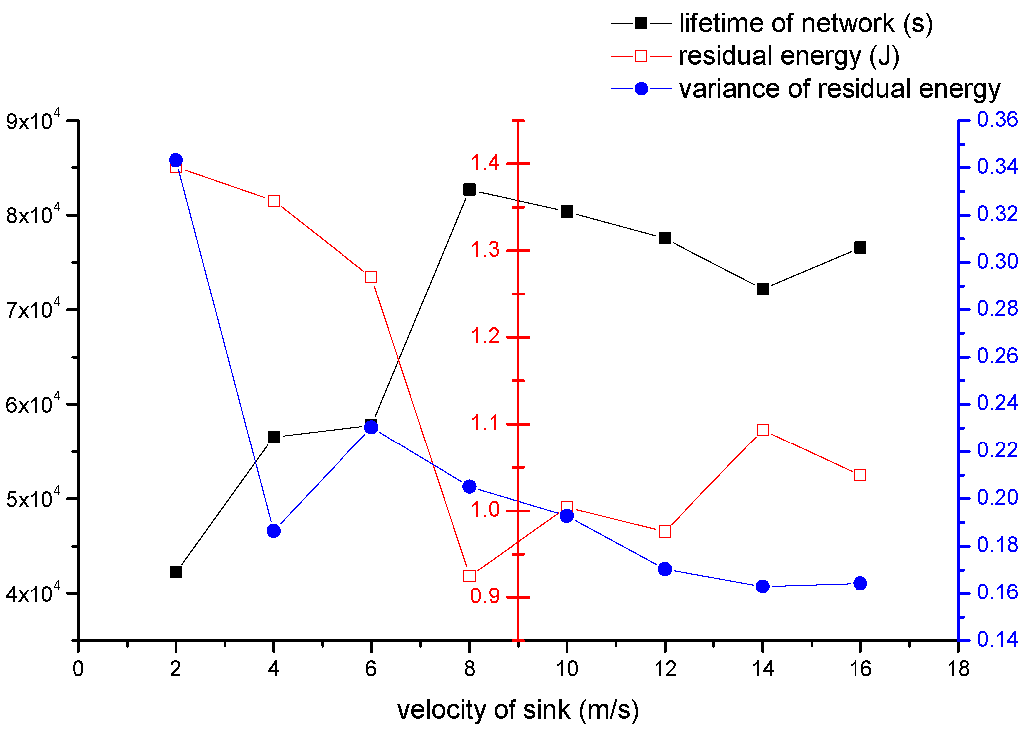
4.2.5. The Impact of Velocity of Sink
4.3. Comparison with VGDRA
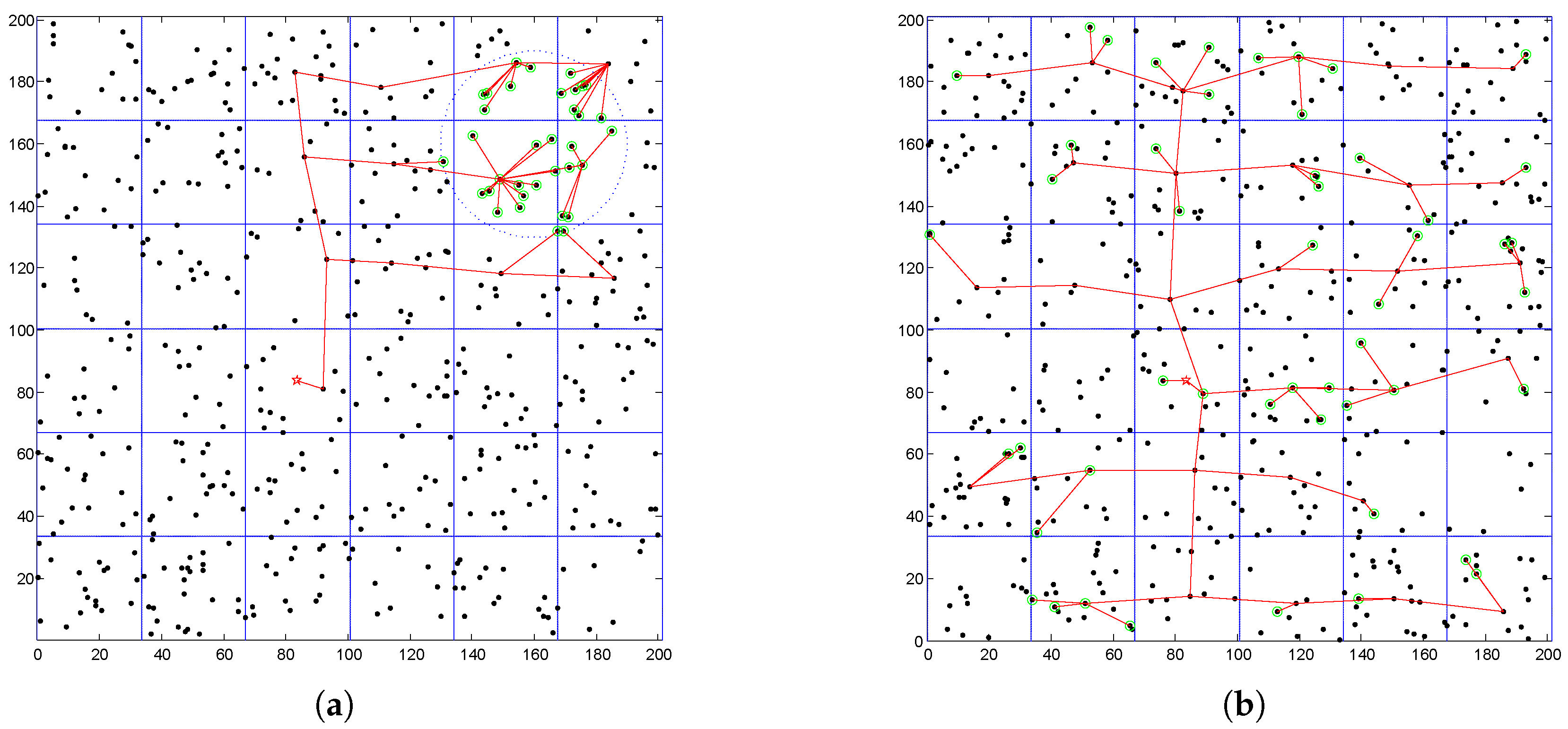
4.3.1. Source Nodes Are Distributed Unevenly in the Network
4.3.2. Source Nodes Are Distributed Evenly in the Network
4.3.3. Only the Energy Consumption of Updating Routes Is Considered
5. Conclusions
Acknowledgments
Author Contributions
Conflicts of Interest
References
- Quang, P.T.A.; Kim, D.S. Enhancing real-time delivery of gradient routing for industrial wireless sensor networks. IEEE Trans. Ind. Inform. 2012, 8, 61–68. [Google Scholar] [CrossRef]
- Han, G.; Liu, L.; Jiang, J.; Shu, L.; Hancke, G. Analysis of energy-efficient connected target coverage algorithms for industrial wireless sensor networks. IEEE Trans. Ind. Inform. 2016. [Google Scholar] [CrossRef]
- Zhao, M.; Yang, Y. Bounded relay hop mobile data gathering in wireless sensor networks. IEEE Trans. Comput. 2012, 61, 265–277. [Google Scholar] [CrossRef]
- Tseng, Y.C.; Wu, F.J.; Lai, W.T. Opportunistic data collection for disconnected wireless sensor networks by mobile mules. Ad Hoc Netw. 2013, 11, 1150–1164. [Google Scholar] [CrossRef]
- Dong, M.; Ota, K.; Liu, A. RMER: Reliable and Energy Efficient Data Collection for Large-scale Wireless Sensor Networks. IEEE Internet Things J. 2016, 3, 511–519. [Google Scholar] [CrossRef]
- Han, G.; Jiang, J.; Zhang, C.; Duong, T.; Guizani, M.; Karagiannidis, G. A Survey on Mobile Anchor Node Assisted Localization in Wireless Sensor Networks. IEEE Commun. Surv. Tutor. 2016, 18, 2220–2243. [Google Scholar] [CrossRef]
- Shen, J.; Tan, H.W.; Wang, J.; Wang, J.W.; Lee, S.Y. A novel routing protocol providing good transmission reliability in underwater sensor networks. J. Internet Technol. 2015, 16, 171–178. [Google Scholar]
- Xie, S.; Wang, Y. Construction of tree network with limited delivery latency in homogeneous wireless sensor networks. Wireless Pers. Commun. 2014, 78, 231–246. [Google Scholar] [CrossRef]
- Zhang, Y.; Sun, X.; Wang, B. Efficient Algorithm for K-Barrier Coverage Based on Integer Linear Programming. China Commun. 2016, 13, 16–23. [Google Scholar] [CrossRef]
- Guo, P.; Wang, J.; Li, B.; Lee, S.Y. A Variable Threshold-value Authentication Architecture for Wireless Mesh Networks. J. Internet Technol. 2014, 15, 929–936. [Google Scholar]
- Han, G.; Dong, Y.; Guo, H.; Shu, L.; Wu, D. Cross-layer optimized routing in wireless sensor networks with duty cycle and energy harvesting. Wirel. Commun. Mob. Comput. 2015, 15, 1957–1981. [Google Scholar] [CrossRef]
- Han, G.; Qian, A.; Jiang, J.; Sun, N.; Liu, L. A grid-based joint routing and charging algorithm for industrial wireless rechargeable sensor networks. Comput. Netw. 2016, 101, 19–28. [Google Scholar] [CrossRef]
- Dong, M.; Ota, K.; Yang, L. T.; Liu, A.; Guo, M. LSCD: A Low-Storage Clone Detection Protocol for Cyber-Physical Systems. IEEE Trans. Comput.-Aided Des. Integr. Circuits Syst. 2016, 35, 712–723. [Google Scholar] [CrossRef]
- Zhu, C.; Zhang, H.; Han, G.; Shu, L.; Rodrigues, J.J. BTDGS: Binary-Tree based Data Gathering Scheme with Mobile Sink for Wireless Multimedia Sensor Networks. Mob. Netw. Appl. 2015, 20, 604–622. [Google Scholar] [CrossRef]
- Rao, J.; Biswas, S. Analyzing multi-hop routing feasibility for sensor data harvesting using mobile sinks. J. Parallel Distrib. Comput. 2012, 72, 764–777. [Google Scholar] [CrossRef]
- Salarian, H.; Chin, K.W.; Naghdy, F. An energy-efficient mobile-sink path selection strategy for wireless sensor networks. IEEE Trans. Veh. Technol. 2014, 63, 2407–2419. [Google Scholar] [CrossRef]
- Zhu, C.; Wu, S.; Han, G.; Shu, L.; Wu, H. A Tree-Cluster-Based Data-Gathering Algorithm for Industrial WSNs With a Mobile Sink. IEEE Access 2015, 3, 381–396. [Google Scholar] [CrossRef]
- Ma, M.; Yang, Y.; Zhao, M. Tour planning for mobile data-gathering mechanisms in wireless sensor networks. IEEE Trans. Veh. Technol. 2013, 62, 1472–1483. [Google Scholar] [CrossRef]
- Zhao, M.; Yang, Y.; Wang, C. Mobile data gathering with load balanced clustering and dual data uploading in wireless sensor networks. IEEE Trans. Mob. Comput. 2015, 14, 770–785. [Google Scholar] [CrossRef]
- Kinalis, A.; Nikoletseas, S.; Patroumpa, D.; Rolim, J. Biased sink mobility with adaptive stop times for low latency data collection in sensor networks. Inf. Fusion 2014, 15, 56–63. [Google Scholar] [CrossRef]
- Kumar, A.K.; Sivalingam, K.M.; Kumar, A. On reducing delay in mobile data collection based wireless sensor networks. Wirel. Netw. 2013, 19, 285–299. [Google Scholar] [CrossRef]
- Tashtarian, F.; Moghaddam, M.H.Y.; Sohraby, K.; Effati, S. On Maximizing the Lifetime of Wireless Sensor Networks in Event-Driven Applications With Mobile Sinks. IEEE Trans. Veh. Technol. 2015, 64, 3177–3189. [Google Scholar] [CrossRef]
- Tashtarian, F.; Moghaddam, M.Y.; Sohraby, K.; Effati, S. ODT: Optimal deadline-based trajectory for mobile sinks in WSN: A decision tree and dynamic programming approach. Comput. Netw. 2015, 77, 128–143. [Google Scholar] [CrossRef]
- Khan, A.W.; Abdullah, A.H.; Razzaque, M.A.; Bangash, J.I. VGDRA: A virtual grid-based dynamic routes adjustment scheme for mobile sink-based wireless sensor networks. IEEE Sens. J. 2015, 15, 526–534. [Google Scholar] [CrossRef]
- Shin, K.; Kim, S. Predictive routing for mobile sinks in wireless sensor networks: A milestone-based approach. J. Supercomput. 2012, 62, 1519–1536. [Google Scholar] [CrossRef]
- Luo, H.; Ye, F.; Cheng, J.; Lu, S.; Zhang, L. TTDD: Two-tier data dissemination in large-scale wireless sensor networks. Wirel. Netw. 2005, 11, 161–175. [Google Scholar] [CrossRef]
- Tunca, C.; Isik, S.; Donmez, M.Y.; Ersoy, C. Ring routing: An energy-efficient routing protocol for wireless sensor networks with a mobile sink. IEEE Trans. Mob. Comput. 2015, 14, 1947–1960. [Google Scholar] [CrossRef]
- Chen, X.; Xu, M. A geographical cellular-like architecture for wireless sensor networks. In Proceedings of the First International Conference on Mobile Ad-Hoc and Sensor Networks, Wuhan, China, 13–15 December 2005; pp. 249–258.
- Chen, T.S.; Tsai, H.W.; Chang, Y.H.; Chen, T.C. Geographic convergecast using mobile sink in wireless sensor networks. Comput. Commun. 2013, 36, 445–458. [Google Scholar] [CrossRef]
- Han, S.W.; Jeong, I.S.; Kang, S.H. Low latency and energy efficient routing tree for wireless sensor networks with multiple mobile sinks. J. Netw. Comput. Appl. 2013, 36, 156–166. [Google Scholar] [CrossRef]
- Ahmadi, M.; He, L.; Pan, J.; Xu, J. A partition-based data collection scheme for wireless sensor networks with a mobile sink. In Proceedings of the 2012 IEEE International Conference on Communications (ICC), Ottawa, ON, Canada, 10–15 June 2012; pp. 503–507.
- Liu, X.; Zhao, H.; Yang, X.; Li, X. SinkTrail: A proactive data reporting protocol for wireless sensor networks. IEEE Trans. Comput. 2013, 62, 151–162. [Google Scholar] [CrossRef]
- Mir, Z.H.; Ko, Y.B. A quadtree-based hierarchical data dissemination for mobile sensor networks. Telecommun. Syst. 2007, 36, 117–128. [Google Scholar] [CrossRef]
- Shi, L.; Yao, Z.; Zhang, B.; Li, C.; Ma, J. An efficient distributed routing protocol for wireless sensor networks with mobile sinks. Int. J. Commun. Syst. 2015, 28, 1789–1804. [Google Scholar] [CrossRef]
- Shin, J.H.; Park, D. A virtual infrastructure for large-scale wireless sensor networks. Comput. Commun. 2007, 30, 2853–2866. [Google Scholar] [CrossRef]
- Heinzelman, W.B.; Chandrakasan, A.P.; Balakrishnan, H. An application-specific protocol architecture for wireless microsensor networks. IEEE Trans. Wirel. Commun. 2002, 1, 660–670. [Google Scholar] [CrossRef]
- Manjeshwar, A.; Agrawal, D.P. TEEN: A Routing Protocol for Enhanced Efficiency in Wireless Sensor Networks. In Proceedings of the 15th International Parallel and Distributed Processing Symposium, San Francisco, CA, USA, 23–27 April 2000.
- Shi, G.; Zheng, J.; Yang, J.; Zhao, Z. Double-blind data discovery using double cross for large-scale wireless sensor networks with mobile sinks. IEEE Trans. Veh. Technol. 2012, 61, 2294–2304. [Google Scholar]
- Yuan, X.X.; Zhang, R.H. An energy-efficient mobile sink routing algorithm for wireless sensor networks. In Proceedings of the 7th International Conference on Wireless Communications, Networking and Mobile Computing (WiCOM), Wuhan, China, 23–25 September 2011; pp. 1–4.
- Zhao, H.; Guo, S.; Wang, X.; Wang, F. Energy-efficient topology control algorithm for maximizing network lifetime in wireless sensor networks with mobile sink. Appl. Soft. Comput. 2015, 34, 539–550. [Google Scholar] [CrossRef]
- Mottaghi, S.; Zahabi, M.R. Optimizing LEACH clustering algorithm with mobile sink and rendezvous nodes. AEU—Int. J. Electron. Commun. 2015, 69, 507–514. [Google Scholar] [CrossRef]
- Konstantopoulos, C.; Pantziou, G.; Gavalas, D.; Mpitziopoulos, A.; Mamalis, B. A rendezvous-based approach enabling energy-efficient sensory data collection with mobile sinks. IEEE Trans. Parallel Distrib. Syst. 2012, 23, 809–817. [Google Scholar] [CrossRef]
- He, L.; Pan, J.; Xu, J. A progressive approach to reducing data collection latency in wireless sensor networks with mobile elements. IEEE Trans. Mob. Comput. 2013, 12, 1308–1320. [Google Scholar] [CrossRef]
- Handcock, R.N.; Swain, D.L.; Bishop-Hurley, G.J.; Patison, K.P.; Wark, T.; Valencia, P. Monitoring animal behaviour and environmental interactions using wireless sensor networks, GPS collars and satellite remote sensing. Sensors 2009, 9, 3586–3603. [Google Scholar] [CrossRef] [PubMed]
- Akbas, M.I.; Brust, M.R.; Ribeiro, C.H.; Turgut, D. fAPEbook-animal social life monitoring with wireless sensor and actor networks. In Proceedings of the 2011 IEEE Global Telecommunications Conference, Houston, TX, USA, 5–9 December 2011; pp. 1–5.
- Mainwaring, A.; Culler, D.; Polastre, J.; Szewczyk, R.; Anderson, J. Wireless sensor networks for habitat monitoring. In Proceedings of the 1st ACM international workshop on Wireless sensor networks and applications, Atlanta, GA, USA, 28 September 2002; pp. 88–97.
- Younis, O.; Fahmy, S. HEED: A hybrid, energy-efficient, distributed clustering approach for ad hoc sensor networks. IEEE Trans. Mob. Comput. 2004, 3, 366–379. [Google Scholar] [CrossRef]


| Categories | References | Advantages | Disadvantages | |
|---|---|---|---|---|
| Uploading pattern | Passive uploading | [3,4,16,17,18,19,20,21,22,23] | Lower energy consumption | (1) Long latency of data collection (2) High pressure on memory of nodes |
| Active uploading | [14,24,25,26,27,28,29] | Real time | (1) Hard to update sink’s current location quickly with lower energy consumption (2) Fast energy consumption around sink | |
| Organization pattern | Non-virtual structure based | [16,25,30] | Network model is easy to established | The way to find current location of sink is inefficient |
| Virtual structure based | [14,20,24,26,27,28,29,31,32,33,34,35] | (1) Nodes are well organized (2) Source nodes are easy to get sink’s location | Maintenance of some virtual structure is complex | |
| Moving pattern | Mobility without purpose | [14,24,25,26,27,28,29,38,39,40,41,42] | Simple system maintenance | Cannot adapt to the dynamic changes of network |
| Mobility with purpose | [3,16,17,18,19,20,22,32,43] | Good flexibility | Maintenance of system is not simple | |
| Notation | Definition |
|---|---|
| Sensing radius of nodes | |
| a | Side length of a grid cell |
| v | Speed of the mobile sink |
| N | Number of nodes deployed in network |
| R | Communication radius of nodes |
| L | Longitudinal length of network |
| Initial coordinate of the mobile sink | |
| Coordinate of node deployed in network |
| coordinate of the upside neighbor head node | |
| coordinate of the downside neighbor head node | |
| coordinate of the left side neighbor head node | |
| coordinate of the right side neighbor head node |
| Criterion/Condition | Category |
|---|---|
| Value | Direction to Transmission | Column Selected in Neighbor Table |
|---|---|---|
| 1 | left | |
| 2 | right | |
| 3 | down | |
| 4 | up | |
| 0 | (broadcast in local grid) | (broadcast in local grid) |
| Parameters | Definition | Default Settings |
|---|---|---|
| L | Side length of deployment area | 200 m |
| N | Number of sensor nodes | 200∼600 |
| Node communication radius | 75 m | |
| Radius of event area | 20∼60 m | |
| E | Initial energy of each node | 2 J |
| Threshold of communication | 75 m | |
| Digital electronics | 50 nJ/bit | |
| Communication | 10 pJ/bit/m2 | |
| Communication | 0.0013 pJ/bi/m4 |
© 2016 by the authors; licensee MDPI, Basel, Switzerland. This article is an open access article distributed under the terms and conditions of the Creative Commons Attribution (CC-BY) license (http://creativecommons.org/licenses/by/4.0/).
Share and Cite
Zhu, C.; Zhang, S.; Han, G.; Jiang, J.; Rodrigues, J.J.P.C. A Greedy Scanning Data Collection Strategy for Large-Scale Wireless Sensor Networks with a Mobile Sink. Sensors 2016, 16, 1432. https://doi.org/10.3390/s16091432
Zhu C, Zhang S, Han G, Jiang J, Rodrigues JJPC. A Greedy Scanning Data Collection Strategy for Large-Scale Wireless Sensor Networks with a Mobile Sink. Sensors. 2016; 16(9):1432. https://doi.org/10.3390/s16091432
Chicago/Turabian StyleZhu, Chuan, Sai Zhang, Guangjie Han, Jinfang Jiang, and Joel J. P. C. Rodrigues. 2016. "A Greedy Scanning Data Collection Strategy for Large-Scale Wireless Sensor Networks with a Mobile Sink" Sensors 16, no. 9: 1432. https://doi.org/10.3390/s16091432
APA StyleZhu, C., Zhang, S., Han, G., Jiang, J., & Rodrigues, J. J. P. C. (2016). A Greedy Scanning Data Collection Strategy for Large-Scale Wireless Sensor Networks with a Mobile Sink. Sensors, 16(9), 1432. https://doi.org/10.3390/s16091432