
Conditional Random Field-Based Offline Map Matching for Indoor Environments

 ,
,  and
and
Abstract
:1. Introduction
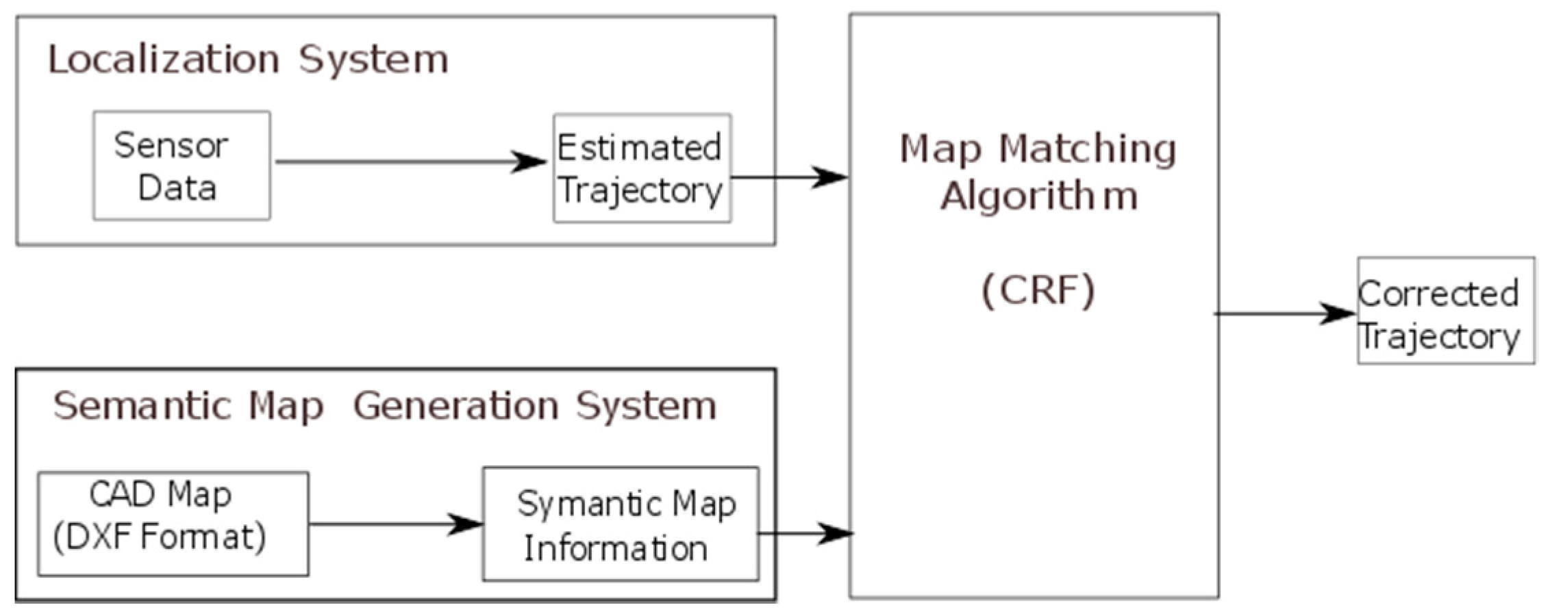
2. Overview of the System
- The primary localization system that produces the first estimated trajectory. This can be any localization system that produces, as its output, a walking trajectory in the form of a time sequence of estimated location coordinates. This trajectory will be the input of the map matching algorithm.
- The semantic map generation system, a unit that models the floor plan obtained from CAD files in a semantic format that can be used by the map matching algorithm. In our case, a grid-based map model was employed in which the floor plan map is divided into square uniform-grid cells. Each cell is associated with a semantic representation of its contents, for example if it contains a wall or a free space.
- The map matching algorithm that refines the estimated trajectory (path) using the CRF technique and the semantic floor plan information.
2.1. The Semantic Map Generation System
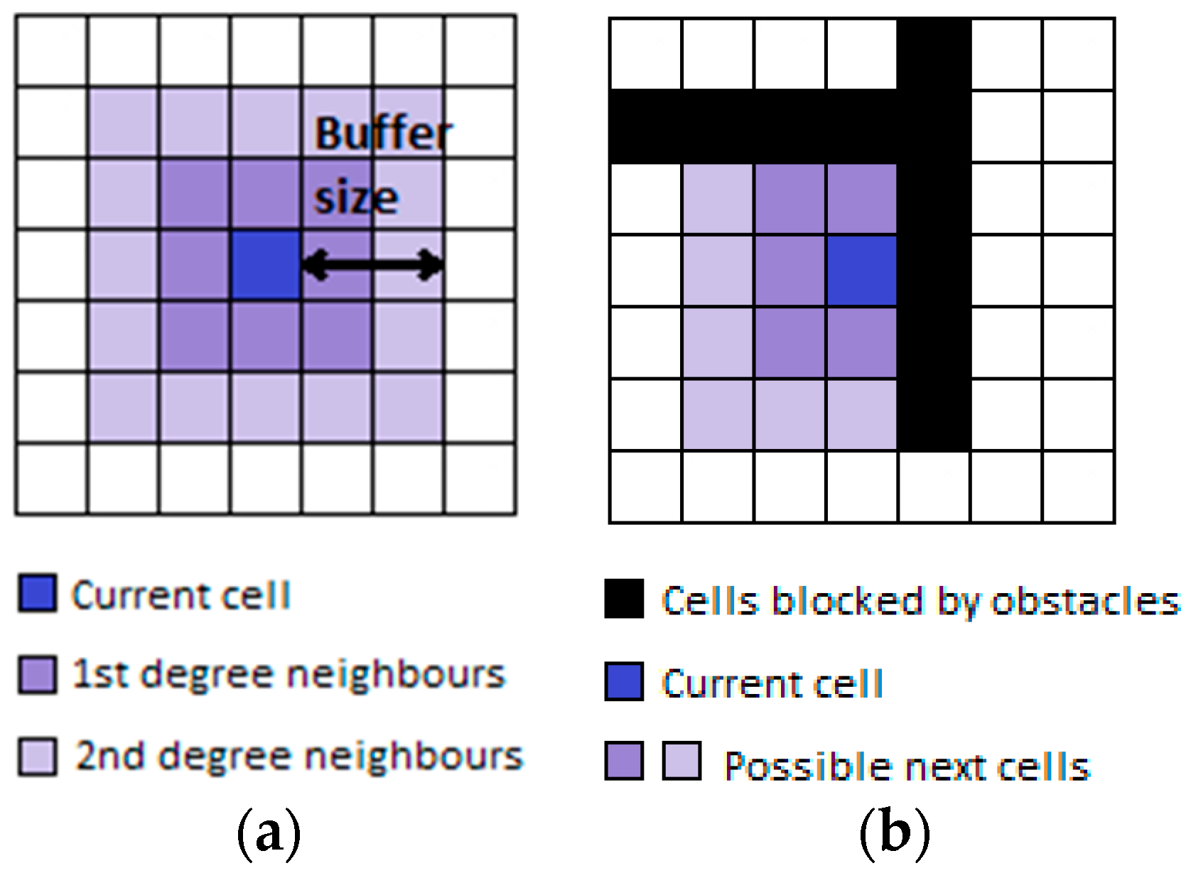
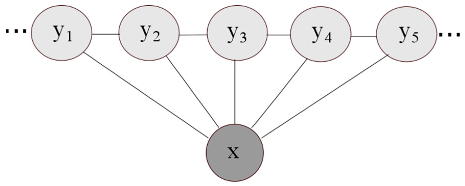
2.2. The Map Matching Algorithm
| Algorithm 1. CRF Algorithm for the Map Matching Problem | |
| 1 | Input : Observation = a vector of coordinates of the input estimated trajectory |
| 2 | Output: CorrectedPath = a vector of coordinates of the output corrected trajectory |
| 3 | Forward Phase: |
| 4 | For each observation (Observationj) %Observation j = coordinates of the input at time step j |
| 5 | For all cells (i) |
| 6 | For all neighbor cells of i (k) |
| 7 | fdis = T(i,k)/Distance (k,Observationj)%T(i,k): transition possibility from cell i to cell k {0,1} |
| 8 | Potential(k,Observationj) = exp(fdis); |
| 9 | Z = sum(Potential(:,j)) % normalization factor |
| 10 | ConditionalProbabilty (k,Observationj) = Potential(k,Observationj)/Z |
| 11 | If (ConditionalProbabilty (i,Observationj-1) > ConditionalProbabilty (bestParent (k)) |
| 12 | then CorrectedParent(k) = i |
| 13 | End |
| 14 | End |
| 15 | End |
| 16 | End |
| 17 | Backward Phase |
| 18 | #CandidatePaths = #Cells |
| 19 | For p = 1➜ #CandidatePaths % p is the last cell in the CandidatePaths |
| 20 | k = p % k is the current cell in the CandidatePath |
| 21 | Construct each CandidatePath: |
| 22 | For all observations (j ➜1) |
| 23 | CandidatePath(j) = k; %add cell K to the path at time step j |
| 24 | sum(CandidatePath) = sum(CandidatePath) + ConditionalProbabilty(k,j) |
| 25 | k = BestParent(k,j) % choose the best parent of k to be the next cell in the path |
| 26 | End |
| 27 | End |
| 28 | CorrectedPath = CandidatePath with highest sum of ConditionalProbabilities |
3. Results and Discussion
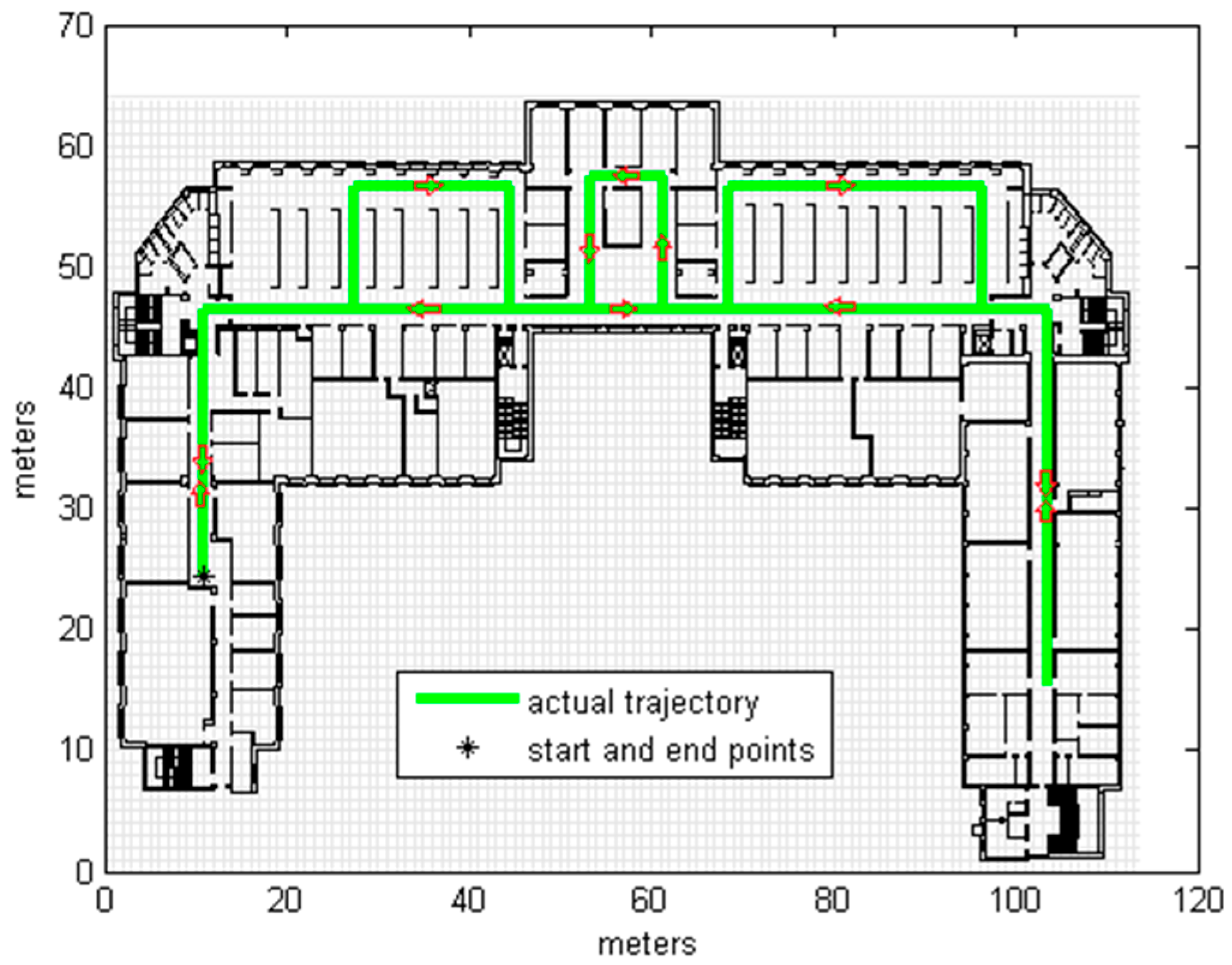
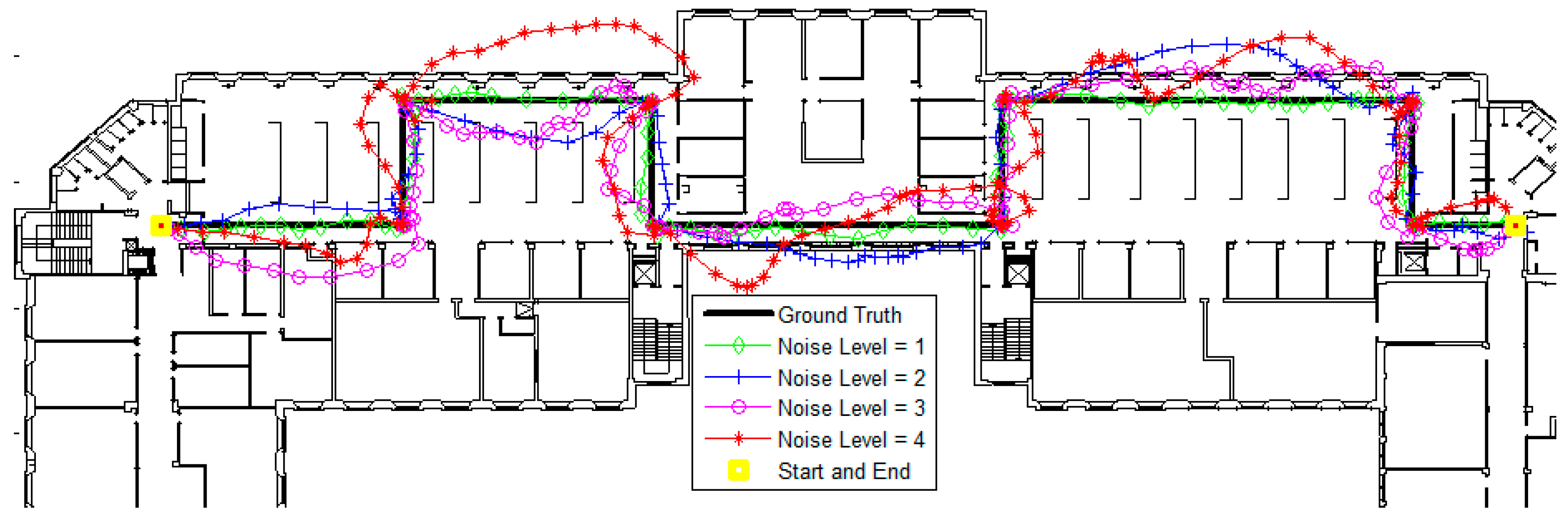
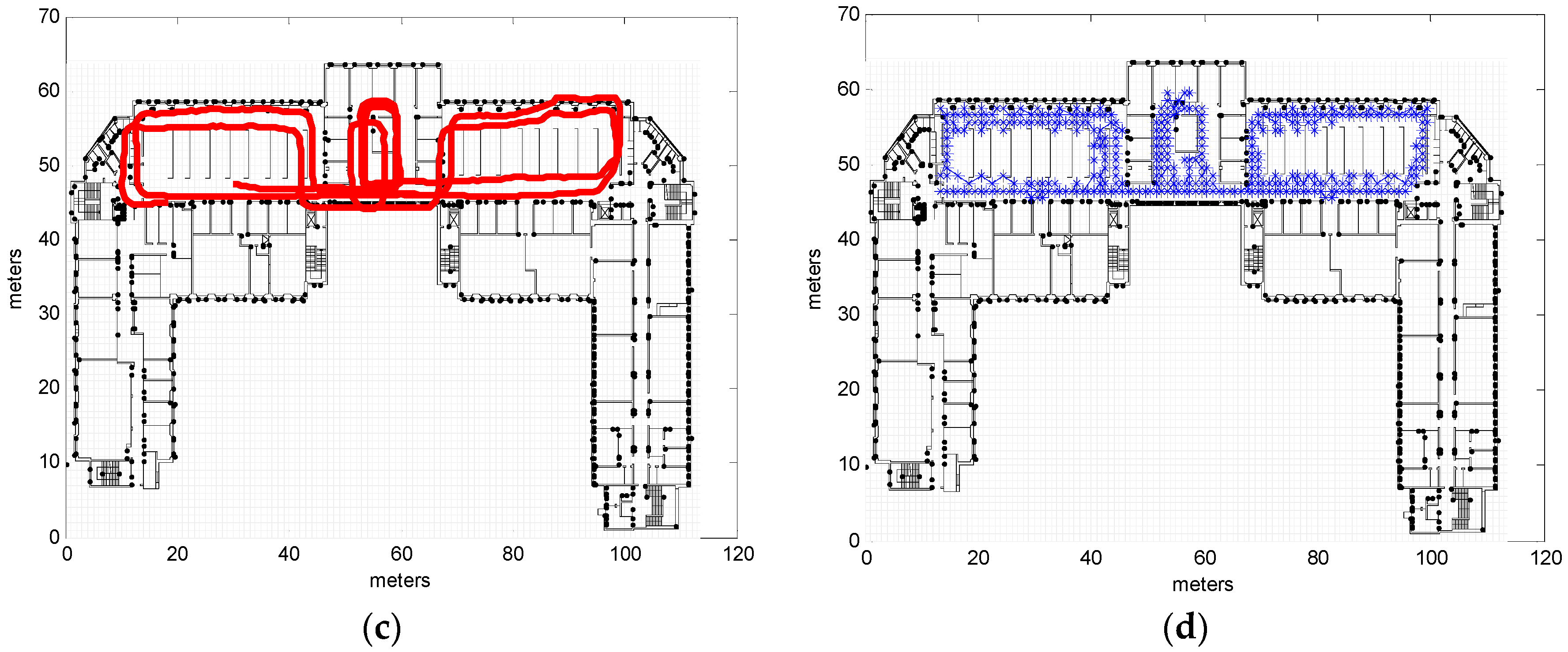
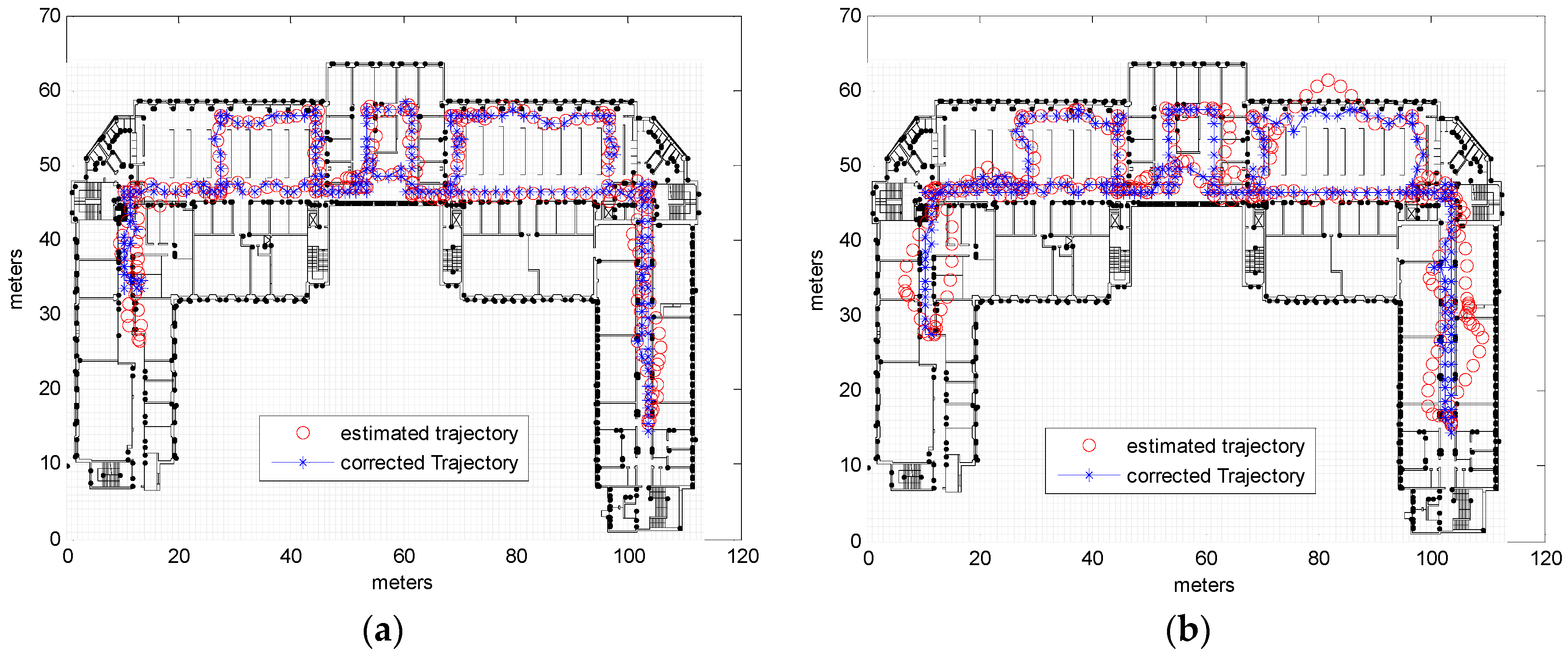
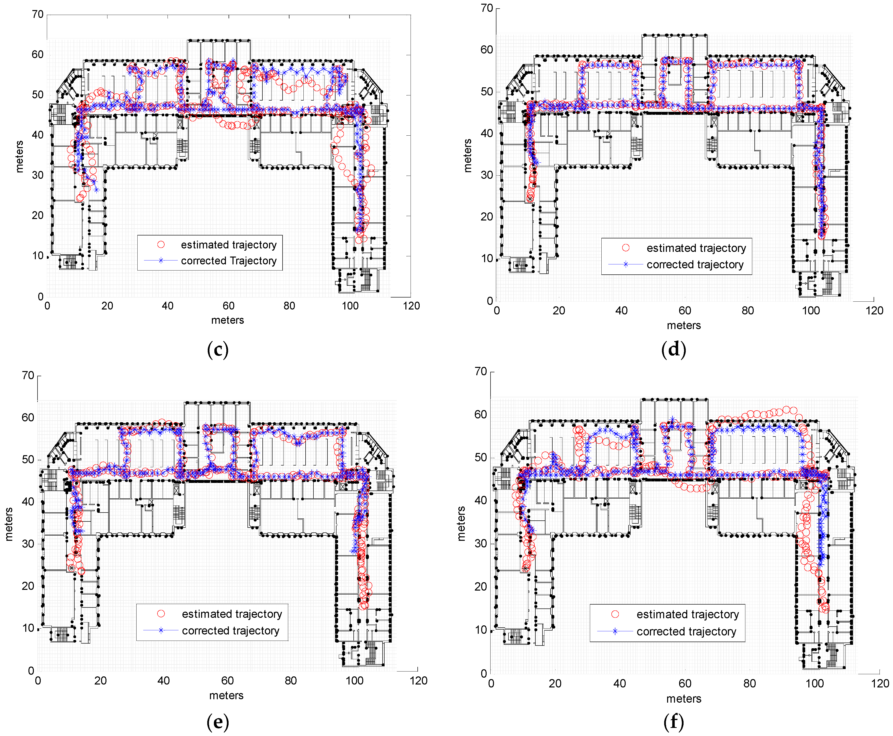
3.1. Simulations
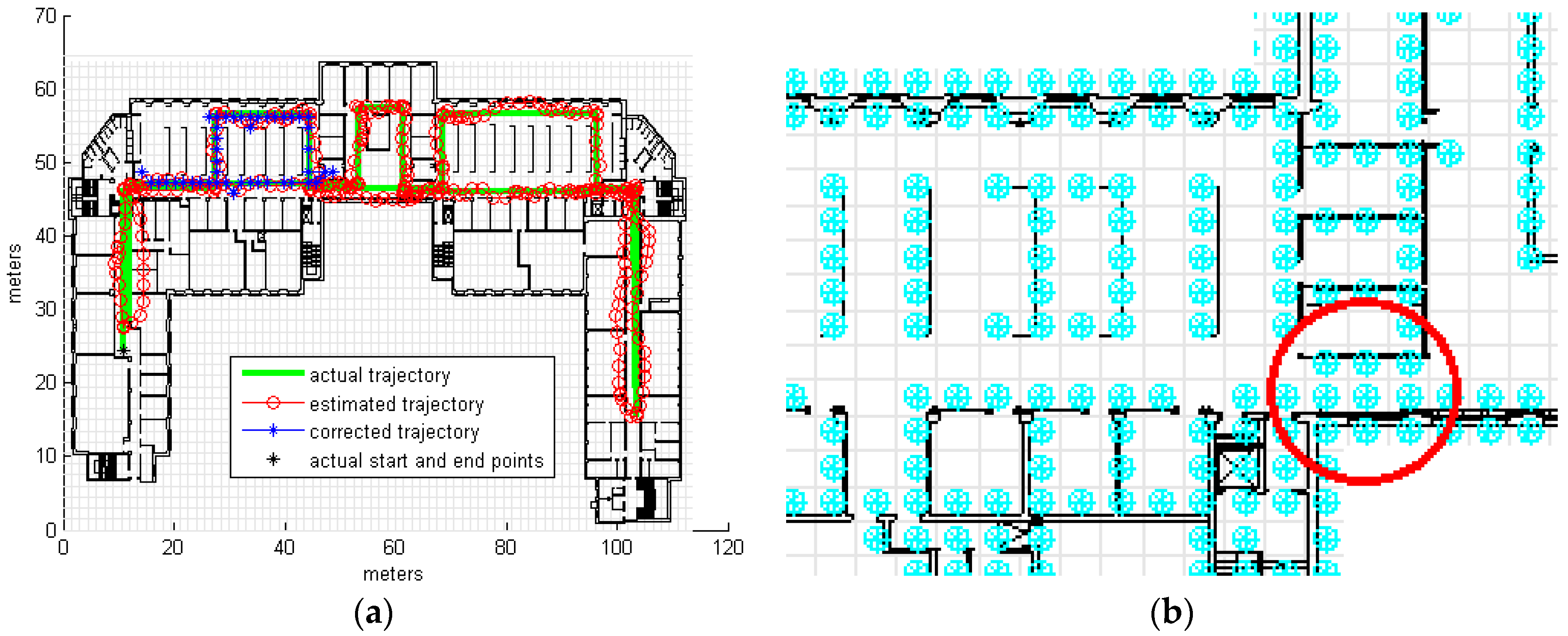
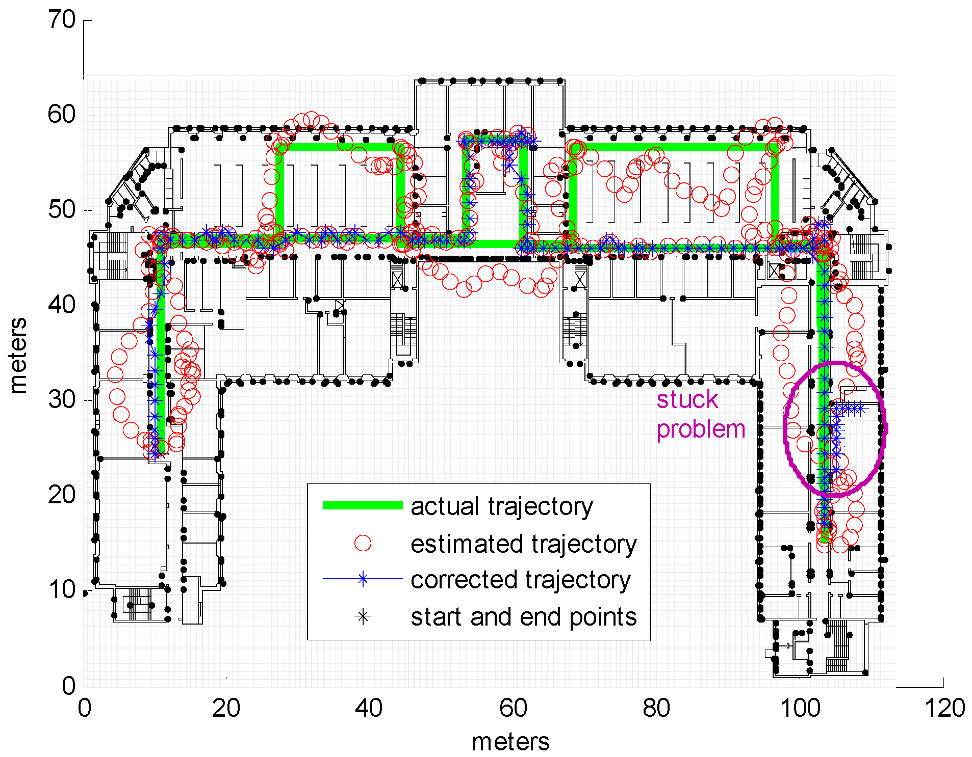
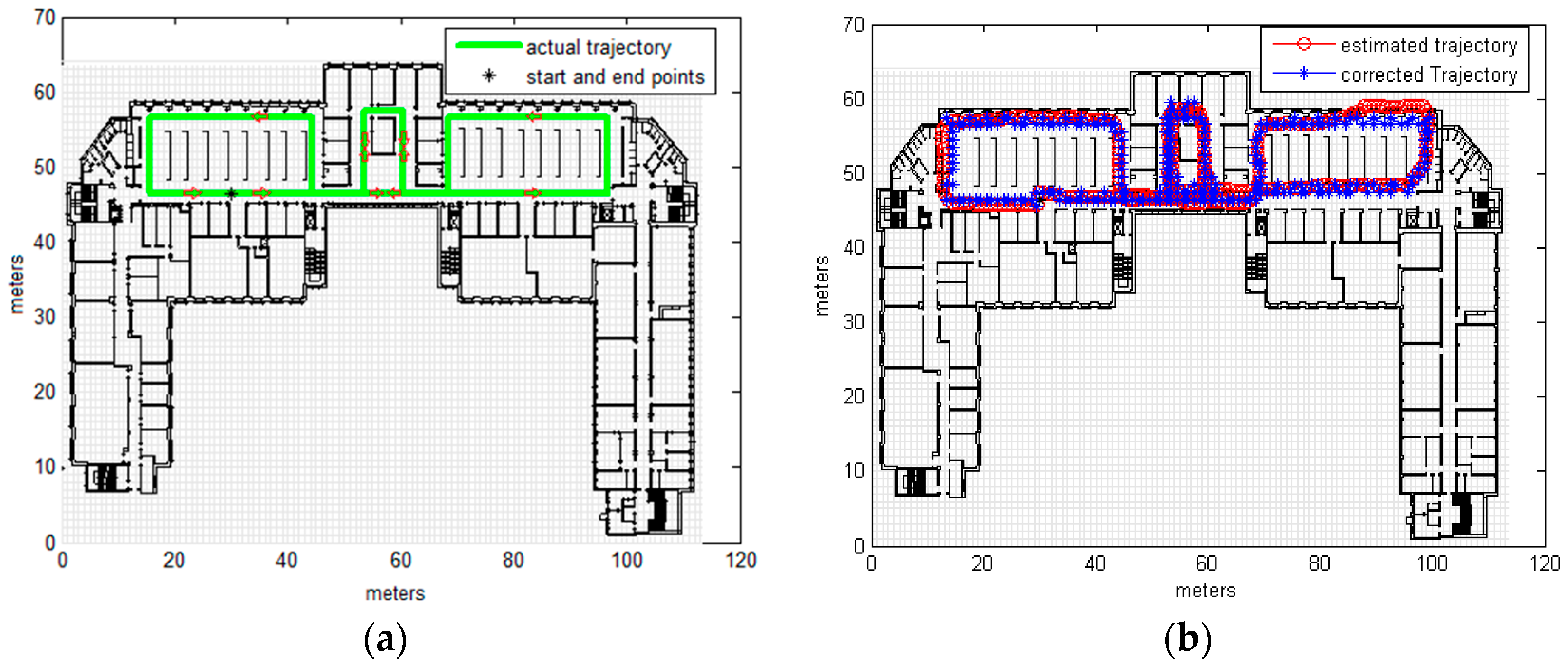
3.2. Real Measurements
4. Conclusions
Acknowledgments
Author Contributions
Conflicts of Interest
Abbreviations
| GNSS | Global Navigation Satellite System |
| CRF | Conditional Random Fields |
| HMM | Hidden Marcov Models |
| PDR | Pedestrian Dead-Reckoning |
| DXF | Drawing Interchange file format |
| CDF | Cumulative Distribution Function |
| iHDE | improved Heuristic Drift Elimination |
References
- Klepeis, N.E.; Nelson, W.C.; Ott, W.R.; Robinson, J.P.; Tsang, A.M.; Switzer, P.; Behar, J.V.; Hern, S.C.; Engelmann, W.H. The National Human Activity Pattern Survey (NHAPS): A resource for assessing exposure to environmental pollutants. J. Expo. Anal. Environ. Epidemiol. 2001, 11, 231–252. [Google Scholar] [CrossRef] [PubMed]
- Shang, J.; Hu, X.; Gu, F.; Wang, D.; Yu, S. Improvement Schemes for Indoor Mobile Location Estimation: A Survey. Math. Probl. Eng. 2015, 2015, 397298. [Google Scholar] [CrossRef]
- Quddus, M.A.; Ochieng, W.Y.; Noland, R.B. Current map matching algorithms for transport applications: State-of-the art and future research directions. Transp. Res. C Emerg. Technol. 2007, 15, 312–328. [Google Scholar] [CrossRef]
- Arulampalam, M.S.; Maskell, S.; Gordon, N.; Clapp, T. A tutorial on particle filters for online nonlinear/non-Gaussian Bayesian tracking. IEEE Trans. Signal Process. 2002, 50, 174–188. [Google Scholar] [CrossRef]
- Davidson, P.; Collin, J.; Takala, J. Application of particle filters for indoor positioning using floor plans. In Ubiquitous Positioning Indoor Navigation and Location Based Service (UPINLBS); IEEE: New York, NY, USA, 2010; pp. 1–4. [Google Scholar]
- Klepal, M.; Pesch, D. A bayesian approach for rf-based indoor localization. In Proceedings of the 4th International Symposium on Wireless Communication Systems ISWCS, Trondheim, Norway, 17–19 October 2007; pp. 133–137.
- Klepal, M.; Beauregard, S. A backtracking particle filter for fusing building plans with PDR displacement estimates. In Proceedings of the 5th Workshop on Positioning, Navigation and Communication WPNC, Hannover, Germany, 27 March 2008; pp. 207–212.
- Klinger, R.; Tomanek, K. Classical Probabilistic Models and Conditional Random Fields; Algorithm Engineering TU: North Rhine-Westphalia, Germany, 2007. [Google Scholar]
- Lafferty, J.; McCallum, A.; Pereira, F.C. Conditional random fields: Probabilistic models for segmenting and labeling sequence data. In Proceedings of the 18th International Conference on Machine Learning, Williamstown, MA, USA, 28 June–1 July 2001.
- Ramos, F.T.; Fox, D.; Durrant-Whyte, H.F. CRF-Matching: Conditional Random Fields for Feature-Based Scan Matching. In Robotics: Science and Systems III; MIT Press: Cambridge, MA, USA, 2007. [Google Scholar]
- Pereira, F.C.; Costa, H.; Pereira, N.M. An off-line map matching algorithm for incomplete map databases. Eur. Tranp. Res. Rev. 2009, 1, 107–124. [Google Scholar] [CrossRef]
- Xiao, Z.; Wen, H.; Markham, A.; Trigoni, N. Lightweight map matching for indoor localization using conditional random fields. In Proceedings of the 13th International Symposium on Information Processing in Sensor Networks IPSN-14, Berlin, Germany, 15–17 April 2014; pp. 131–142.
- Xu, M.; Du, Y.; Wu, J.; Zhou, Y. Map Matching Based on Conditional Random Fields and Route Preference Mining for Uncertain Trajectories. Math. Probl. Eng. 2015, 2015, 717095. [Google Scholar] [CrossRef]
- Lamarche, F.; Donikian, S. Crowd of virtual humans: A new approach for real time navigation in complex and structured environments. In Computer Graphics Forum; Blackwell Publishing, Inc.: Oxford, UK, 2014; pp. 509–518. [Google Scholar]
- Drawing Interchange and File Formats, Release 12. Available online: http://cnc25.free.fr/documentation/format_dxf/dxf.pdf (accessed on 22 March 2016).
- Autodesk, Inc. (n.d.) Drawing Interchange File Formats. Available online: http://www.autodesk.com/techpubs/autocad/acadr14/dxf/drawing_interchange_file_formats.htm (accessed on 22 March 2016).
- Schäfer, M.; Knapp, C.; Chakraborty, S. Automatic generation of topological indoor maps for real-time map-based localization and tracking. In Proceedings of the 2011 International Conference on Indoor Positioning and Indoor Navigation (IPIN), Guimaraes, Portugal, 21–23 September 2011; pp. 1–8.
- Jordan, A. On discriminative vs. generative classifiers: A comparison of logistic regression and naive bayes. Adv. Neural Inform. Process. Syst. 2002, 14, 841. [Google Scholar]
- Forney, G.D., Jr. The viterbi algorithm. In Proceedings of the IEEE; IEEE: New York, NY, USA, 1973; Volume 61, pp. 268–278. [Google Scholar]
- Elsevier Health Sciences. Moderate Intensity Walking Means 100 Steps Per Minute. ScienceDaily. 21 March 2009. Available online: www.sciencedaily.com/releases/2009/03/090317094719.htm (accessed on 22 April 2016).
- Determine Your Stride. Available online: https://cdn.shopify.com/s/files/1/0196/4616/files/Soleus-determing_your_stride.pdf (accessed on 23 April 2016).
- Diez, L.E.; Bahillo, A.; Bataineh, S.; Masegosa, A.D. Enhancing Improved Heuristic Drift Elimination for Wrist-Worn PDR Systems in Buildings. In Proceedings of the IEEE Vehicular Technology Conference, Nanjing, China, 15–18 May 2016.


| Noise Level | Mean (m) | Standard Deviation (m) |
|---|---|---|
| 1 | 1.3 | 1 |
| 2 | 1.6 | 1.1 |
| 3 | 2.0 | 1.3 |
| 4 | 2.5 | 1.8 |
| Cell Size (m) | Noise Level | Number of Crossed Obstacles | Cumulative Error (m) | |
|---|---|---|---|---|
| 50% | 90% | |||
| 0.8 | 1 | 0 | 0.9867 | 2.6699 |
| 2 | 0 | 2.682 | 19.7820 | |
| 3 | 0 | 5.7945 | 32.464 | |
| 4 | 0 | 6.5158 | 32.3861 | |
| 1 | 1 | 0 | 1.1574 | 3.078 |
| 2 | 0 | 1.2463 | 3.8172 | |
| 3 | 0 | 1.4853 | 5.1879 | |
| 4 | 0 | 2.1409 | 11.1061 | |
| 1.5 | 1 | 0 | 19.4403 | 70.7003 |
| 2 | 0 | 16.6941 | 61.6751 | |
| 3 | 0 | 17.7461 | 68.5491 | |
| 4 | 0 | 20.0473 | 71.8129 | |
| Estimation Frequency | Buffer Size | Cumulative Error (Meters) | |
|---|---|---|---|
| 50% | 90% | ||
| 1 Hz | 1 cell | 12.4931 | 33.1054 |
| 2 Hz | 1 cell | 1.1348 | 2.4989 |
| 1 Hz | 2 cells | 1.1574 | 3.078 |
| 2 Hz | 2 cells | 1.3639 | 3.0044 |
| Algorithm | Number of Crossed Obstacles | Cumulative Error (m) | |
|---|---|---|---|
| 50% | 90% | ||
| iHDE | 15 | 1.2861 | 2.6858 |
| iHDE + CRF | 0 | 1.0634 | 2.2316 |
© 2016 by the authors; licensee MDPI, Basel, Switzerland. This article is an open access article distributed under the terms and conditions of the Creative Commons Attribution (CC-BY) license (http://creativecommons.org/licenses/by/4.0/).
Share and Cite
Bataineh, S.; Bahillo, A.; Díez, L.E.; Onieva, E.; Bataineh, I. Conditional Random Field-Based Offline Map Matching for Indoor Environments. Sensors 2016, 16, 1302. https://doi.org/10.3390/s16081302
Bataineh S, Bahillo A, Díez LE, Onieva E, Bataineh I. Conditional Random Field-Based Offline Map Matching for Indoor Environments. Sensors. 2016; 16(8):1302. https://doi.org/10.3390/s16081302
Chicago/Turabian StyleBataineh, Safaa, Alfonso Bahillo, Luis Enrique Díez, Enrique Onieva, and Ikram Bataineh. 2016. "Conditional Random Field-Based Offline Map Matching for Indoor Environments" Sensors 16, no. 8: 1302. https://doi.org/10.3390/s16081302
APA StyleBataineh, S., Bahillo, A., Díez, L. E., Onieva, E., & Bataineh, I. (2016). Conditional Random Field-Based Offline Map Matching for Indoor Environments. Sensors, 16(8), 1302. https://doi.org/10.3390/s16081302