
An Analysis on Sensor Locations of the Human Body for Wearable Fall Detection Devices: Principles and Practice

Abstract
:
1. Introduction
2. System Design
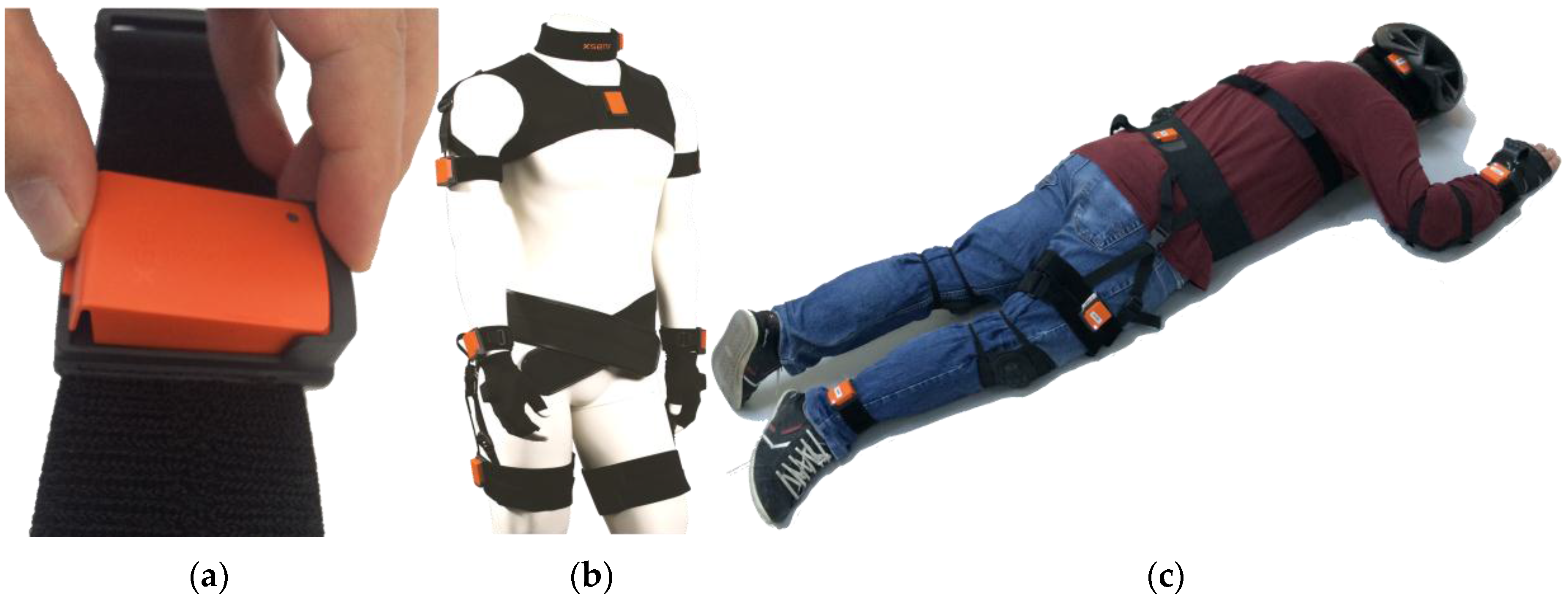
2.1. Dataset, Volunteers and Tests
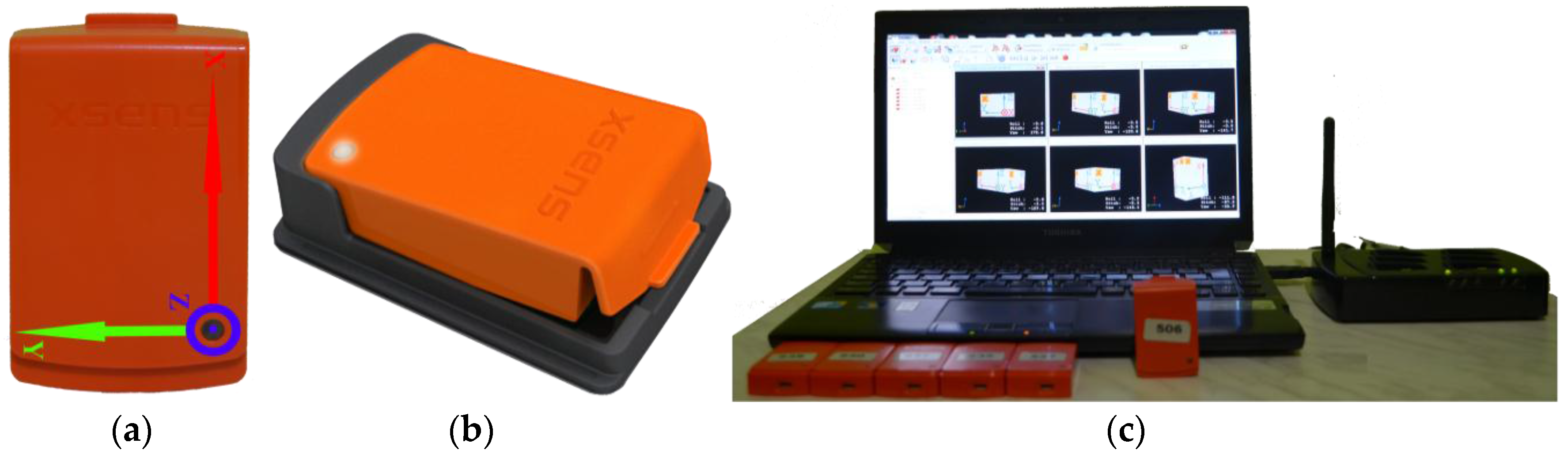
2.2. Sensor Specifications
2.3. Experimental Setup
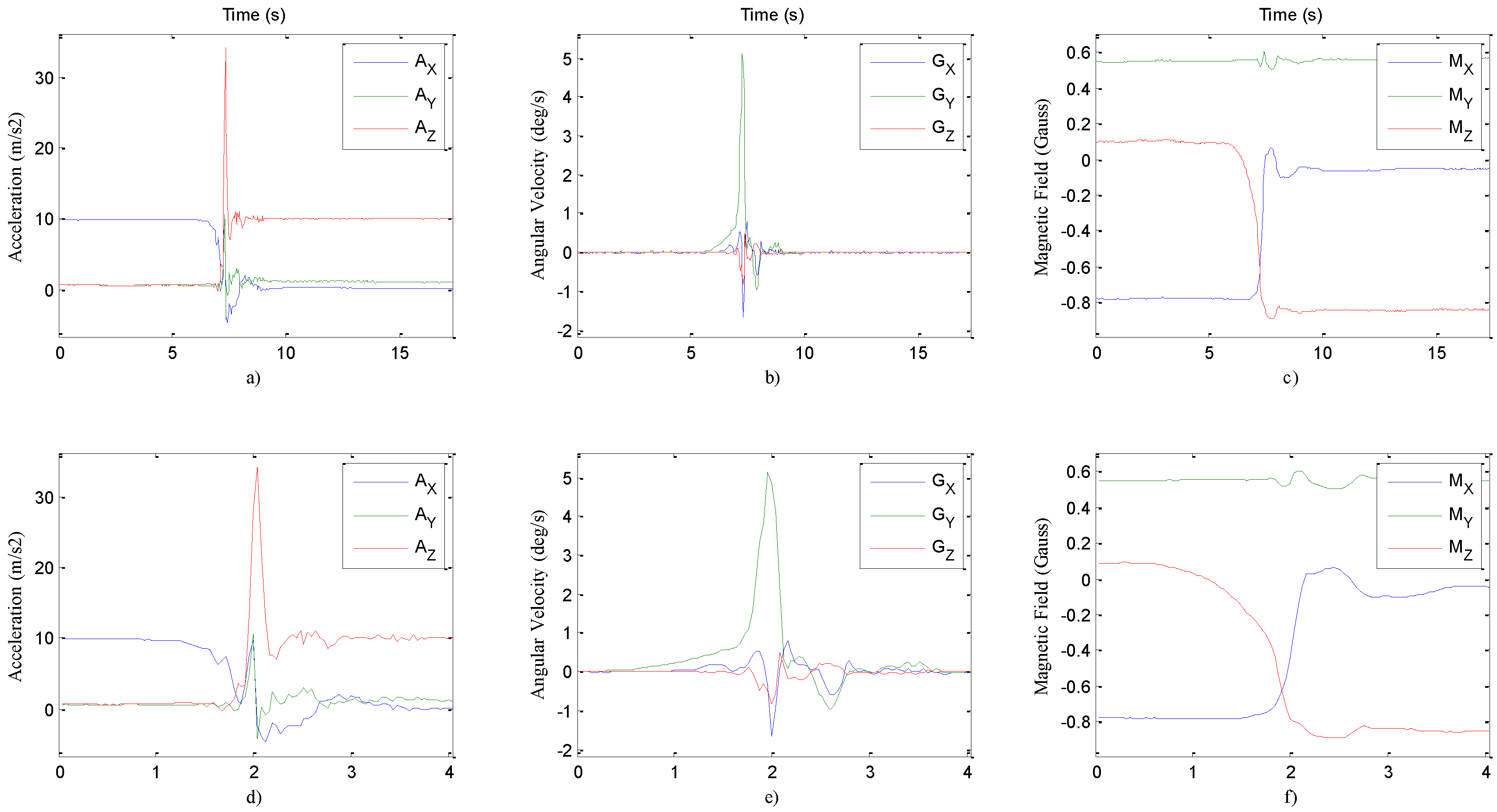
2.4. Data Formation
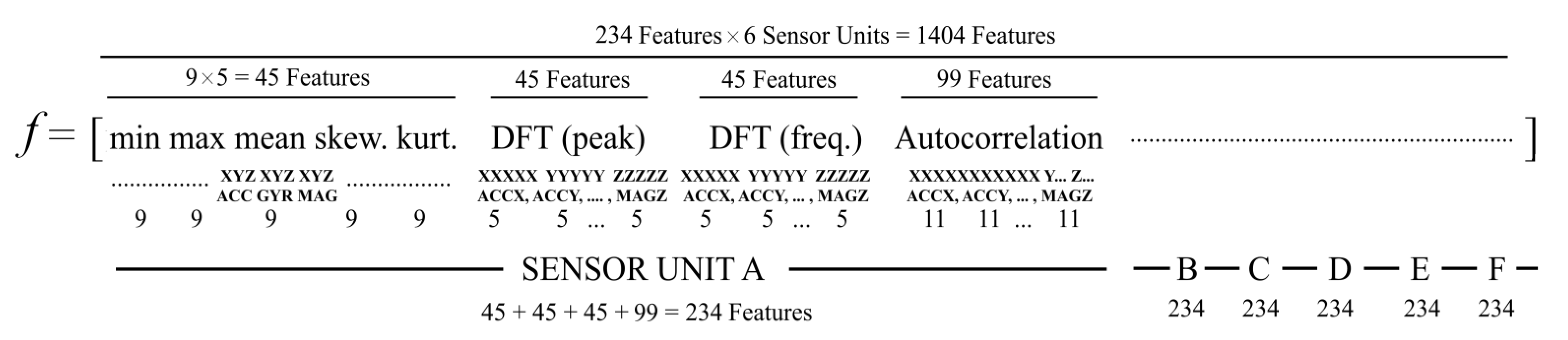
2.5. Feature Extraction and Dimensional Reduction
3. Materials and Methods
3.1. The k-Nearest Neighbor Classifier
3.2. Bayesian Decision Making
3.3. Support Vector Machines
3.4. Least Squares Method
3.5. Dynamic Time Warping
3.6. Artificial Neural Networks
4. Results and Discussion
5. Conclusions
Acknowledgments
Conflicts of Interest
References
- Custodio, V.; Herrera, F.J.; López, G.; Moreno, J.I. A review on architectures and communications technologies for wearable health-monitoring systems. Sensors 2012, 12, 13907–13946. [Google Scholar] [CrossRef] [PubMed]
- Chu, N.N.; Yang, C.M.; Wu, C.C. Game interface using digital textile sensors, accelerometer and gyroscope. IEEE Trans. Consum. Electron. 2012, 58, 184–189. [Google Scholar] [CrossRef]
- Moustafa, H.; Kenn, H.; Sayrafian, K.; Scanlon, W.; Zhang, Y. Mobile wearable communications. IEEE Wirel. Commun. 2015, 22, 10–11. [Google Scholar] [CrossRef]
- Patel, S.; Park, H.; Bonato, P.; Chan, L.; Rodgers, M. A review of wearable sensors and systems with application in rehabilitation. J. Neuroeng. Rehabil. 2012, 9, 1–17. [Google Scholar] [CrossRef] [PubMed]
- Borthwick, A.C.; Anderson, C.L.; Finsness, E.S.; Foulger, T.S. Special article personal wearable technologies in education: Value or villain? J. Digit. Learn. Teacher Educ. 2015, 31, 85–92. [Google Scholar] [CrossRef]
- Rubenstein, L.Z. Falls in older people: Epidemiology, risk factors and strategies for prevention. Age Ageing 2006, 35, ii37–ii41. [Google Scholar] [CrossRef] [PubMed]
- Lord, S.R.; Sherrington, C.; Menz, H.B.; Close, J.C. Falls in Older People: Risk Factors and Strategies for Prevention; Cambridge University Press: Cambridge, UK, 2007. [Google Scholar]
- Mahoney, J.E.; Eisner, J.; Havighurst, T.; Gray, S.; Palta, M. Problems of older adults living alone after hospitalization. J. Gen. Intern. Med. 2000, 15, 611–619. [Google Scholar] [CrossRef] [PubMed]
- Sattin, R.W.; Huber, D.A.L.; Devito, C.A.; Rodriguez, J.G.; Ros, A.; Bacchelli, S.; Stevens, J.A.; Waxweiler, R.J. The incidence of fall injury events among the elderly in a defined population. Am. J. Epidemiol. 1990, 131, 1028–1037. [Google Scholar] [PubMed]
- Mubashir, M.; Shao, L.; Seed, L. A survey on fall detection: Principles and approaches. Neurocomputing 2013, 100, 144–152. [Google Scholar] [CrossRef]
- Delahoz, Y.; Labrador, M. Survey on fall detection and fall prevention using wearable and external sensors. Sensors 2014, 14, 19806–19842. [Google Scholar] [CrossRef] [PubMed]
- Fortino, G.; Graviana, R. Fall-MobileGuard: A Smart Real-Time Fall Detection System. In Proceedings of the 10th EAI International Conference on Body Area Networks, Sydney, Australia, 28–30 December 2015; pp. 44–50.
- Özdemir, A.T.; Barshan, B. Detecting falls with wearable sensors using machine learning techniques. Sensors 2014, 14, 10691–10708. [Google Scholar] [CrossRef] [PubMed]
- Vavoulas, G.; Pediaditis, M.; Chatzaki, C.; Spanakis, E.G.; Tsiknakis, M. The mobifall dataset: Fall detection and classification with a smartphone. Int. J. Monit. Surveill. Technol. Res. 2014, 2, 44–56. [Google Scholar] [CrossRef]
- Noury, N.; Rumeau, P.; Bourke, A.; ÓLaighin, G.; Lundy, J. A proposal for the classification and evaluation of fall detectors. IRBM 2008, 29, 340–349. [Google Scholar] [CrossRef]
- Bagalà, F.; Becker, C.; Cappello, A.; Chiari, L.; Aminian, K.; Hausdorff, J.M.; Zijlstra, W.; Klenk, J. Evaluation of accelerometer-based fall detection algorithms on real-world falls. PLoS ONE 2012, 7, e37062. [Google Scholar] [CrossRef] [PubMed]
- Noury, N.; Fleury, A.; Rumeau, P.; Bourke, A.; Laighin, G.; Rialle, V.; Lundy, J. Fall detection-principles and methods. In Proceedings of the 29th Annual International Conference of the IEEE Engineering in Medicine and Biology Society, Lyon, France, 23–26 August 2007; pp. 1663–1666.
- Kangas, M.; Konttila, A.; Lindgren, P.; Winblad, I.; Jämsä, T. Comparison of low-complexity fall detection algorithms for body attached accelerometers. Gait Posture 2008, 28, 285–291. [Google Scholar] [CrossRef] [PubMed]
- Li, Q.; Stankovic, J.; Hanson, M.; Barth, A.T.; Lach, J.; Zhou, G. Accurate, fast fall detection using gyroscopes and accelerometer-derived posture information. In Proceedings of the IEEE 6th International Workshop on Wearable and Implantable Body Sensor Networks, Berkerey, CA, USA, 3–5 June 2009; pp. 138–143.
- Atallah, L.; Lo, B.; King, R.; Yang, G.-Z. Sensor placement for activity detection using wearable accelerometers. In Proceedings of the IEEE Body Sensor Networks (BSN), Singapore, 7–9 June 2010; pp. 24–29.
- Bao, L.; Intille, S.S. Activity recognition from user-annotated acceleration data. In Pervasive Computing; Springer: Vienna, Austria, 2004; pp. 1–17. [Google Scholar]
- Shi, G.; Zhang, J.; Dong, C.; Han, P.; Jin, Y.; Wang, J. Fall detection system based on inertial mems sensors: Analysis design and realization. In Proceedings of the IEEE International Conference on Cyber Technology in Automation, Control, and Intelligent Systems, Shenyang, China, 8–12 June 2015; pp. 1834–1839.
- De Backere, F.; Ongenae, F.; Van den Abeele, F.; Nelis, J.; Bonte, P.; Clement, E.; Philpott, M.; Hoebeke, J.; Verstichel, S.; Ackaert, A. Towards a social and context-aware multi-sensor fall detection and risk assessment platform. Comput. Biol. Med. 2014, 64, 307–320. [Google Scholar] [CrossRef] [PubMed]
- Finlayson, M.L.; Peterson, E.W. Falls, aging, and disability. Phys. Med. Rehabil. Clin. N. Am. 2010, 21, 357–373. [Google Scholar] [CrossRef] [PubMed]
- Abbate, S.; Avvenuti, M.; Corsini, P.; Light, J.; Vecchio, A. Monitoring of human movements for fall detection and activities recognition in elderly care using wwireless sensor network: A survey. In Application-Centric Design Book, 1st ed.; InTech: Rijeka, Croatia, 2010; Chapter 9; pp. 147–166. [Google Scholar]
- MTw Development Kit User Manual and Technical Documentation. Xsens Technologies B.V.: Enschede, The Netherlands, 2016. Available online: http://www.xsens.com (accessed on 20 June 2016).
- Barshan, B.; Yüksek, M.C. Recognizing daily and sports activities in two open source machine learning environments using body-worn sensor units. Comput. J. 2013, 57, 1649–1667. [Google Scholar] [CrossRef]
- Altun, K.; Barshan, B.; Tuncel, O. Comparative study on classifying human activities with miniature inertial and magnetic sensors. Pattern Recogn. 2010, 43, 3605–3620. [Google Scholar] [CrossRef]
- Chan, M.; Campo, E.; Bourennane, W.; Estève, D. Connectivity for the indoor and outdoor elderly people safety management: An example from our current project. In Proceedings of the 7th European Symposium on Biomedical Engineering, Chalkidiki, Greece, 28–29 May 2010.
- Wu, G.; Cavanagh, P.R. ISB recommendations for standardization in the reporting of kinematic data. J. Biomech. 1995, 28, 1257–1261. [Google Scholar] [CrossRef]
- Ozdemir, A.T.; Danisman, K. A comparative study of two different FPGA-based arrhythmia classifier architectures. Turk. J. Electr. Eng. Comput. 2015, 23, 2089–2106. [Google Scholar] [CrossRef]
- Wang, C.; Lu, W.; Narayanan, M.R.; Redmond, S.J.; Lovell, N.H. Low-power technologies for wearable telecare and telehealth systems: A review. Biomed. Eng. Lett. 2015, 5, 1–9. [Google Scholar] [CrossRef]
- Chaudhuri, S.; Kneale, L.; Le, T.; Phelan, E.; Rosenberg, D.; Thompson, H.; Demiris, G. Older adults' perceptions of fall detection devices. J. Appl. Gerontol. 2016, 71. [Google Scholar] [CrossRef] [PubMed]
- Duda, R.O.; Hart, P.E.; Stork, D.G. Pattern Classification, 2nd ed.; Wiley: New York, NY, USA, 2001. [Google Scholar]
- Chang, C.C.; Lin, C.J. LibSVM: A library for support vector machines. ACM Trans. Intell. Syst. Technol. 2011, 2, 1–27. [Google Scholar] [CrossRef]
- Keogh, E.; Ratanamahatana, C.A. Exact indexing of dynamic time warping. Knowl. Inf. Syst. 2005, 7, 358–386. [Google Scholar] [CrossRef]
- University of Irvine Machine Learning Repository. Available online: http://archive.ics.uci.edu/ml/ (accessed on 20 June 2016).


| Men | Women | All | |||||||||||||
|---|---|---|---|---|---|---|---|---|---|---|---|---|---|---|---|
| Volunteers | 101 | 102 | 103 | 104 | 106 | 107 | 108 | 203 | 204 | 205 | 206 | 207 | 208 | 209 | Ave. |
| Age | 21 | 21 | 23 | 27 | 22 | 21 | 21 | 21 | 21 | 20 | 19 | 20 | 24 | 22 | 21.64 |
| Height (kg) | 75 | 81 | 78 | 67 | 54 | 72 | 68 | 51 | 47 | 51 | 47 | 60 | 55 | 70 | 62.57 |
| Weight (cm) | 170 | 174 | 180 | 176 | 160 | 175 | 184 | 170 | 157 | 169 | 166 | 165 | 163 | 182 | 170.79 |
| Activities of Daily Living (ADLs) | Voluntary Falls | ||||
|---|---|---|---|---|---|
| # | Label | Description | # | Label | Description |
| 801 | Walking fw | Walking forward | 901 | Front lying | From vertical going forward to the floor |
| 802 | Walking bw | Walking backward | 902 | Front protected lying | From vertical going forward to the floor with arm protection |
| 803 | Jogging | Running | 903 | Front knees | From vertical going down on the knees |
| 804 | Squatting down | Going down, then up | 904 | Front knees lying | From vertical going down on the knees and then lying on the floor |
| 805 | Bending | Bending of about 90 degrees | 905 | Front quick recovery | From vertical going on the floor and quick recovery |
| 806 | Bending and pick up | Bending to pick up an object on the floor | 906 | Front slow recovery | From vertical going on the floor and slow recovery |
| 807 | Limp | Walking with a limp | 907 | Front right | From vertical going down on the floor, ending in right lateral position |
| 808 | Stumble | Stumbling with recovery | 908 | Front left | From vertical going down on the floor, ending in left lateral position |
| 809 | Trip over | Bending while walking and then continue walking | 909 | Back sitting | From vertical going on the floor, ending sitting |
| 810 | Coughing | Coughing or sneezing | 910 | Back lying | From vertical going on the floor, ending lying |
| 811 | Sit chair | From vertical sitting with a certain acceleration on a chair (hard surface) | 911 | Back right | From vertical going on the floor, ending lying in right lateral position |
| 812 | Sit sofa | From vertical sitting with a certain acceleration on a sofa (soft surface) | 912 | Back left | From vertical going on the floor, ending lying in left lateral position |
| 813 | Sit air | From vertical sitting in the air exploiting the muscles of legs | 913 | Right sideway | From vertical going on the floor, ending lying |
| 814 | Sit bed | From vertical sitting with a certain acceleration on a bed (soft surface) | 914 | Right recovery | From vertical going on the floor with subsequent recovery |
| 815 | Lying bed | From vertical lying on the bed | 915 | Left sideway | From vertical going on the floor, ending lying |
| 816 | Rising bed | From lying to sitting | 916 | Left recovery | From vertical going on the floor with subsequent recovery |
| 917 | Rolling out bed | From lying, rolling out of bed and going on the floor | |||
| 918 | Podium | From vertical standing on a podium going on the floor | |||
| 919 | Syncope | From standing going on the floor following a vertical trajectory | |||
| 920 | Syncope wall | From standing going down slowly slipping on a wall | |||
| SENSORS | SENSORS | ||||||||||||||
|---|---|---|---|---|---|---|---|---|---|---|---|---|---|---|---|
| * | Ankle | Thigh | Wrist | Waist | Chest | Head | COMB | * | Ankle | Thigh | Wrist | Waist | Chest | Head | COMB |
| F | E | D | C | B | A | F | E | D | C | B | A | ||||
| 0 | 0 | 0 | 0 | 0 | 0 | 0 | 32 | 1 | 0 | 0 | 0 | 0 | 0 | F | |
| 1 | 0 | 0 | 0 | 0 | 0 | 1 | A | 33 | 1 | 0 | 0 | 0 | 0 | 1 | AF |
| 2 | 0 | 0 | 0 | 0 | 1 | 0 | B | 34 | 1 | 0 | 0 | 0 | 1 | 0 | BF |
| 3 | 0 | 0 | 0 | 0 | 1 | 1 | AB | 35 | 1 | 0 | 0 | 0 | 1 | 1 | ABF |
| 4 | 0 | 0 | 0 | 1 | 0 | 0 | C | 36 | 1 | 0 | 0 | 1 | 0 | 0 | CF |
| 5 | 0 | 0 | 0 | 1 | 0 | 1 | AC | 37 | 1 | 0 | 0 | 1 | 0 | 1 | ACF |
| 6 | 0 | 0 | 0 | 1 | 1 | 0 | BC | 38 | 1 | 0 | 0 | 1 | 1 | 0 | BCF |
| 7 | 0 | 0 | 0 | 1 | 1 | 1 | ABC | 39 | 1 | 0 | 0 | 1 | 1 | 1 | ABCF |
| 8 | 0 | 0 | 1 | 0 | 0 | 0 | D | 40 | 1 | 0 | 1 | 0 | 0 | 0 | DF |
| 9 | 0 | 0 | 1 | 0 | 0 | 1 | AD | 41 | 1 | 0 | 1 | 0 | 0 | 1 | ADF |
| 10 | 0 | 0 | 1 | 0 | 1 | 0 | BD | 42 | 1 | 0 | 1 | 0 | 1 | 0 | BDF |
| 11 | 0 | 0 | 1 | 0 | 1 | 1 | ABD | 43 | 1 | 0 | 1 | 0 | 1 | 1 | ABDF |
| 12 | 0 | 0 | 1 | 1 | 0 | 0 | CD | 44 | 1 | 0 | 1 | 1 | 0 | 0 | CDF |
| 13 | 0 | 0 | 1 | 1 | 0 | 1 | ACD | 45 | 1 | 0 | 1 | 1 | 0 | 1 | ACDF |
| 14 | 0 | 0 | 1 | 1 | 1 | 0 | BCD | 46 | 1 | 0 | 1 | 1 | 1 | 0 | BCDF |
| 15 | 0 | 0 | 1 | 1 | 1 | 1 | ABCD | 47 | 1 | 0 | 1 | 1 | 1 | 1 | ABCDF |
| 16 | 0 | 1 | 0 | 0 | 0 | 0 | E | 48 | 1 | 1 | 0 | 0 | 0 | 0 | EF |
| 17 | 0 | 1 | 0 | 0 | 0 | 1 | AE | 49 | 1 | 1 | 0 | 0 | 0 | 1 | AEF |
| 18 | 0 | 1 | 0 | 0 | 1 | 0 | BE | 50 | 1 | 1 | 0 | 0 | 1 | 0 | BEF |
| 19 | 0 | 1 | 0 | 0 | 1 | 1 | ABE | 51 | 1 | 1 | 0 | 0 | 1 | 1 | ABEF |
| 20 | 0 | 1 | 0 | 1 | 0 | 0 | CE | 52 | 1 | 1 | 0 | 1 | 0 | 0 | CEF |
| 21 | 0 | 1 | 0 | 1 | 0 | 1 | ACE | 53 | 1 | 1 | 0 | 1 | 0 | 1 | ACEF |
| 22 | 0 | 1 | 0 | 1 | 1 | 0 | BCE | 54 | 1 | 1 | 0 | 1 | 1 | 0 | BCEF |
| 23 | 0 | 1 | 0 | 1 | 1 | 1 | ABCE | 55 | 1 | 1 | 0 | 1 | 1 | 1 | ABCEF |
| 24 | 0 | 1 | 1 | 0 | 0 | 0 | DE | 56 | 1 | 1 | 1 | 0 | 0 | 0 | DEF |
| 25 | 0 | 1 | 1 | 0 | 0 | 1 | ADE | 57 | 1 | 1 | 1 | 0 | 0 | 1 | ADEF |
| 26 | 0 | 1 | 1 | 0 | 1 | 0 | BDE | 58 | 1 | 1 | 1 | 0 | 1 | 0 | BDEF |
| 27 | 0 | 1 | 1 | 0 | 1 | 1 | ABDE | 59 | 1 | 1 | 1 | 0 | 1 | 1 | ABDEF |
| 28 | 0 | 1 | 1 | 1 | 0 | 0 | CDE | 60 | 1 | 1 | 1 | 1 | 0 | 0 | CDEF |
| 29 | 0 | 1 | 1 | 1 | 0 | 1 | ACDE | 61 | 1 | 1 | 1 | 1 | 0 | 1 | ACDEF |
| 30 | 0 | 1 | 1 | 1 | 1 | 0 | BCDE | 62 | 1 | 1 | 1 | 1 | 1 | 0 | BCDEF |
| 31 | 0 | 1 | 1 | 1 | 1 | 1 | ABCDE | 63 | 1 | 1 | 1 | 1 | 1 | 1 | ACBDEF |
| No. | COMB | k-NN | BDM | SVM | LSM | DTW | ANN | No. | COMB | k-NN | BDM | SVM | LSM | DTW | ANN |
|---|---|---|---|---|---|---|---|---|---|---|---|---|---|---|---|
| 0 | NONE | 32 | F | 99.50 | 98.24 | 99.06 | 96.36 | 93.51 | 95.30 | ||||||
| 1 | A | 99.20 | 97.29 | 96.08 | 96.77 | 96.12 | 94.20 | 33 | FA | 99.91 | 99.19 | 99.35 | 99.04 | 97.04 | 95.56 |
| 2 | B | 99.60 | 96.65 | 96.28 | 95.53 | 96.58 | 94.35 | 34 | FB | 99.55 | 98.85 | 99.22 | 98.27 | 96.31 | 95.13 |
| 3 | BA | 99.69 | 98.74 | 98.19 | 98.10 | 97.12 | 95.29 | 35 | FBA | 99.70 | 99.43 | 99.32 | 99.32 | 97.04 | 95.61 |
| 4 | C | 99.87 | 99.24 | 98.99 | 98.46 | 98.29 | 95.69 | 36 | FC | 99.81 | 99.47 | 99.59 | 98.66 | 96.24 | 95.46 |
| 5 | CA | 99.92 | 99.60 | 99.37 | 98.88 | 97.11 | 95.67 | 37 | FCA | 99.93 | 99.74 | 99.55 | 99.38 | 97.41 | 95.55 |
| 6 | CB | 99.77 | 99.23 | 99.00 | 98.13 | 97.35 | 95.63 | 38 | FCB | 99.80 | 99.34 | 99.42 | 99.02 | 97.30 | 95.58 |
| 7 | CBA | 99.76 | 99.54 | 99.37 | 99.17 | 96.84 | 95.82 | 39 | FCBA | 99.83 | 99.53 | 99.62 | 99.59 | 97.52 | 95.70 |
| 8 | D | 97.49 | 96.08 | 95.27 | 94.63 | 93.62 | 92.40 | 40 | FD | 99.60 | 97.88 | 98.92 | 98.35 | 95.63 | 94.50 |
| 9 | DA | 99.65 | 98.52 | 96.72 | 98.56 | 96.99 | 94.29 | 41 | FDA | 99.82 | 98.65 | 98.97 | 99.48 | 97.35 | 95.13 |
| 10 | DB | 99.54 | 98.24 | 97.63 | 96.38 | 94.42 | 94.23 | 42 | FDB | 99.79 | 98.69 | 98.71 | 98.60 | 95.25 | 95.14 |
| 11 | DBA | 99.76 | 98.57 | 98.04 | 98.73 | 96.75 | 95.42 | 43 | FDBA | 99.94 | 99.29 | 99.07 | 99.35 | 97.17 | 95.77 |
| 12 | DC | 99.54 | 98.67 | 98.84 | 98.70 | 97.19 | 94.95 | 44 | FDC | 99.77 | 98.91 | 99.38 | 99.12 | 96.60 | 95.16 |
| 13 | DCA | 99.83 | 99.29 | 99.02 | 99.29 | 97.09 | 95.53 | 45 | FDCA | 99.92 | 99.08 | 99.47 | 99.54 | 98.19 | 95.38 |
| 14 | DCB | 99.66 | 98.75 | 98.82 | 98.60 | 95.86 | 95.08 | 46 | FDCB | 99.85 | 98.85 | 99.16 | 99.00 | 97.41 | 95.31 |
| 15 | DCBA | 99.80 | 99.06 | 99.23 | 99.13 | 97.35 | 95.39 | 47 | FDCBA | 99.85 | 99.16 | 99.37 | 99.48 | 97.40 | 95.92 |
| 16 | E | 99.61 | 99.12 | 99.27 | 98.09 | 95.69 | 95.53 | 48 | FE | 99.75 | 99.15 | 99.57 | 98.18 | 94.79 | 95.54 |
| 17 | EA | 99.81 | 99.13 | 99.52 | 98.39 | 97.37 | 95.53 | 49 | FEA | 99.91 | 99.63 | 99.69 | 99.15 | 96.76 | 95.47 |
| 18 | EB | 99.82 | 99.19 | 99.55 | 98.74 | 96.58 | 95.71 | 50 | FEB | 99.70 | 99.49 | 99.47 | 99.00 | 94.95 | 95.46 |
| 19 | EBA | 99.79 | 99.64 | 99.58 | 99.21 | 97.88 | 96.02 | 51 | FEBA | 99.78 | 99.79 | 99.69 | 99.67 | 97.92 | 95.77 |
| 20 | EC | 99.84 | 99.44 | 99.31 | 98.82 | 95.85 | 95.17 | 52 | FEC | 99.88 | 99.67 | 99.64 | 99.07 | 96.65 | 95.58 |
| 21 | ECA | 99.94 | 99.90 | 99.59 | 98.93 | 97.88 | 95.83 | 53 | FECA | 99.94 | 99.73 | 99.66 | 99.52 | 97.66 | 95.59 |
| 22 | ECB | 99.91 | 99.42 | 99.37 | 99.32 | 96.85 | 95.60 | 54 | FECB | 99.86 | 99.51 | 99.53 | 99.44 | 97.53 | 95.59 |
| 23 | ECBA | 99.88 | 99.67 | 99.62 | 99.31 | 98.11 | 96.27 | 55 | FECBA | 99.86 | 99.65 | 99.67 | 99.56 | 97.40 | 96.18 |
| 24 | ED | 99.63 | 98.60 | 99.29 | 98.41 | 95.62 | 94.93 | 56 | FED | 99.70 | 98.97 | 99.55 | 99.08 | 96.69 | 95.18 |
| 25 | EDA | 99.82 | 99.00 | 99.42 | 98.45 | 97.86 | 95.68 | 57 | FEDA | 99.87 | 99.17 | 99.45 | 99.67 | 98.11 | 95.42 |
| 26 | EDB | 99.77 | 99.04 | 99.38 | 98.77 | 96.41 | 95.30 | 58 | FEDB | 99.83 | 99.25 | 99.21 | 99.25 | 97.27 | 95.36 |
| 27 | EDBA | 99.87 | 99.25 | 99.31 | 99.27 | 97.53 | 95.58 | 59 | FEDBA | 99.90 | 99.30 | 99.38 | 99.48 | 98.02 | 95.63 |
| 28 | EDC | 99.69 | 99.09 | 99.35 | 99.00 | 97.49 | 95.30 | 60 | FEDC | 99.82 | 99.09 | 99.50 | 99.22 | 96.46 | 95.42 |
| 29 | EDCA | 99.88 | 99.22 | 99.56 | 99.45 | 96.69 | 95.72 | 61 | FEDCA | 99.88 | 99.28 | 99.59 | 99.57 | 98.19 | 95.62 |
| 30 | EDCB | 99.84 | 99.05 | 99.40 | 99.13 | 96.72 | 95.51 | 62 | FEDCB | 99.87 | 99.13 | 99.34 | 99.37 | 97.09 | 95.67 |
| 31 | EDCBA | 99.86 | 99.21 | 99.39 | 99.33 | 98.67 | 95.75 | 63 | FEDCBA | 99.91 | 99.26 | 99.48 | 99.65 | 97.85 | 95.68 |
| CONFUSION MATRICES | |||||||||||||||||||
|---|---|---|---|---|---|---|---|---|---|---|---|---|---|---|---|---|---|---|---|
| k-NN | BDM | SVM | LSM | DTW | ANN | ||||||||||||||
| Double | P | N | P | N | P | N | P | N | P | N | P | N | |||||||
| TRUE | P | 1398 | 2 | 1398.5 | 1.5 | 1395.2 | 4.8 | 1387.3 | 12.7 | 1372.5 | 27.5 | 1356.6 | 43.4 | ||||||
| N | 0 | 1120 | 8.6 | 1111.4 | 5.6 | 1114.4 | 11.4 | 1108.6 | 38.7 | 1081.3 | 64.6 | 1055.4 | |||||||
| Acc (%)* | 99.92 | 99.60 | 99.59 | 99.04 | 97.37 | 95.71 | |||||||||||||
| Combinations | CA | CA | FC | FA | EA | EB | |||||||||||||
| Triple | P | N | P | N | P | N | P | N | P | N | P | N | |||||||
| TRUE | P | 1399 | 1 | 1399 | 1 | 1395.1 | 4.9 | 1397 | 3 | 1384 | 16 | 1366.1 | 33.9 | ||||||
| N | 0.4 | 1119.6 | 1.4 | 1118.6 | 3 | 1117 | 10.2 | 1109.8 | 37.4 | 1082.6 | 66.5 | 1053.5 | |||||||
| Acc (%)* | 99.94 | 99.90 | 99.69 | 99.48 | 97.88 | 96.02 | |||||||||||||
| Combinations | ECA | ECA | FEA | FDA | EBA | EBA | |||||||||||||
| Quadruple | P | N | P | N | P | N | P | N | P | N | P | N | |||||||
| TRUE | P | 1400 | 0 | 1398.3 | 1.7 | 1395.4 | 4.6 | 1399.1 | 0.9 | 1381 | 19 | 1368.5 | 31.5 | ||||||
| N | 0.5 | 1118.5 | 3.6 | 1116.4 | 3.1 | 1116.9 | 7.3 | 1112.7 | 26.7 | 1093.3 | 62.4 | 1057.6 | |||||||
| Acc (%)* | 99.94 | 99.79 | 99.69 | 99.67 | 98.19 | 96.27 | |||||||||||||
| Combinations | FDBA | FEBA | FEBA | FEDA | FDCA | ECBA | |||||||||||||
| Quintuple | P | N | P | N | P | N | P | N | P | N | P | N | |||||||
| TRUE | P | 1399.7 | 0.3 | 1398.2 | 1.8 | 1394.8 | 5.2 | 1400 | 0 | 1389.4 | 10.6 | 1367.6 | 32.4 | ||||||
| N | 2.2 | 1117.8 | 7 | 1113 | 3 | 1117 | 10.9 | 1109.1 | 22.9 | 1097.1 | 63.8 | 1056.2 | |||||||
| Acc (%)* | 99.90 | 99.65 | 99.67 | 99.57 | 98.67 | 96.18 | |||||||||||||
| Combinations | FEDBA | FECBA | FECBA | FEDCA | EDCBA | FECBA | |||||||||||||
| CONFUSION MATRICES | |||||||||||||
|---|---|---|---|---|---|---|---|---|---|---|---|---|---|
| k-NN | BDM | SVM | LSM | DTW | ANN | ||||||||
| C (Waist) | P | N | P | N | P | N | P | N | P | N | P | N | |
| TRUE | P | 1399.4 | 0.6 | 1396.2 | 3.8 | 1391.7 | 8.3 | 1395.2 | 4.8 | 1385.6 | 14.4 | 1359.1 | 40.9 |
| N | 2.7 | 1117.3 | 15.3 | 1104.7 | 17.1 | 1102.9 | 34 | 1086 | 28.6 | 1091.4 | 67.8 | 1052.2 | |
| Acc (%)* | 99.87 | 99.24 | 98.99 | 98.46 | 98.29 | 95.69 | |||||||
| E (Thigh) | P | N | P | N | P | N | P | N | P | N | P | N | |
| TRUE | P | 1395.2 | 4.8 | 1390.7 | 9.3 | 1395 | 5 | 1371.5 | 28.5 | 1320.4 | 79.6 | 1354.2 | 45.8 |
| N | 5 | 1115 | 12.8 | 1107.2 | 13.4 | 1106.6 | 19.7 | 1100.3 | 28.9 | 1091.1 | 66.8 | 1053.2 | |
| Acc (%)* | 99.61 | 99.12 | 99.27 | 98.09 | 95.69 | 95.53 | |||||||
| F (Ankle) | P | N | P | N | P | N | P | N | P | N | P | N | |
| TRUE | P | 1392.6 | 7.4 | 1390.6 | 9.4 | 1389.2 | 10.8 | 1326.6 | 73.4 | 1273.1 | 126.9 | 1358.8 | 41.2 |
| N | 5.2 | 1114.8 | 34.9 | 1085.1 | 12.8 | 1107.2 | 18.3 | 1101.7 | 36.6 | 1083.4 | 77.3 | 1042.7 | |
| Acc (%)* | 99.5 | 98.24 | 99.06 | 96.36 | 93.51 | 95.3 | |||||||
| A (Head) | P | N | P | N | P | N | P | N | P | N | P | N | |
| TRUE | P | 1391 | 9 | 1384.6 | 15.4 | 1372.3 | 27.7 | 1376.5 | 23.5 | 1362.2 | 37.8 | 1354.4 | 45.6 |
| N | 11.1 | 1108.9 | 52.9 | 1067.1 | 71 | 1049 | 57.9 | 1062.1 | 60 | 1060 | 100.6 | 1019.4 | |
| ACC | 99.2 | 97.29 | 96.08 | 96.77 | 96.12 | 94.2 | |||||||
| B (Chest) | P | N | P | N | P | N | P | N | P | N | P | N | |
| TRUE | P | 1398.1 | 1.9 | 1380.8 | 19.2 | 1363.9 | 36.1 | 1388.6 | 11.4 | 1381.4 | 18.6 | 1341.1 | 58.9 |
| N | 8.1 | 1111.9 | 65.3 | 1054.7 | 57.6 | 1062.4 | 101.3 | 1018.7 | 67.5 | 1052.5 | 83.5 | 1036.5 | |
| Acc (%)* | 99.6 | 96.65 | 96.28 | 95.53 | 96.58 | 94.35 | |||||||
| D (Wrist) | P | N | P | N | P | N | P | N | P | N | P | N | |
| TRUE | P | 1370.7 | 29.3 | 1371.9 | 28.1 | 1353.8 | 46.2 | 1302.7 | 97.3 | 1314.2 | 85.8 | 1343 | 57 |
| N | 33.9 | 1086.1 | 70.8 | 1049.2 | 73.1 | 1046.9 | 37.9 | 1082.1 | 75.1 | 1044.9 | 161.6 | 985.4 | |
| Acc (%)* | 97.49 | 96.08 | 95.27 | 94.63 | 93.62 | 92.4 | |||||||
| Run | 1 | 2 | 3 | 4 | 5 | 6 | 7 | 8 | 9 | 10 | AVG | STD |
|---|---|---|---|---|---|---|---|---|---|---|---|---|
| Se (%) | 99.93 | 99.93 | 100 | 99.93 | 99.93 | 100 | 99.93 | 100 | 100 | 99.93 | 99.96 | 0.0369 |
| Acc (%) | 99.88 | 99.88 | 99.92 | 99.76 | 99.88 | 99.92 | 99.88 | 99.84 | 99.84 | 99.88 | 99.87 | 0.0460 |
| Sp (%) | 99.82 | 99.82 | 99.82 | 99.55 | 99.82 | 99.82 | 99.82 | 99.64 | 99.64 | 99.82 | 99.76 | 0.1035 |
| TN | 1118 | 1118 | 1118 | 1115 | 1118 | 1118 | 1118 | 1116 | 1116 | 1118 | 1117.3 | 1.1595 |
| FP | 2 | 2 | 2 | 5 | 2 | 2 | 2 | 4 | 4 | 2 | 2.7 | 1.1595 |
| TP | 1399 | 1399 | 1400 | 1399 | 1399 | 1400 | 1399 | 1400 | 1400 | 1399 | 1399.4 | 0.5164 |
| FN | 1 | 1 | 0 | 1 | 1 | 0 | 1 | 0 | 0 | 1 | 0.6 | 0.5164 |
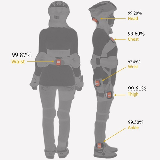
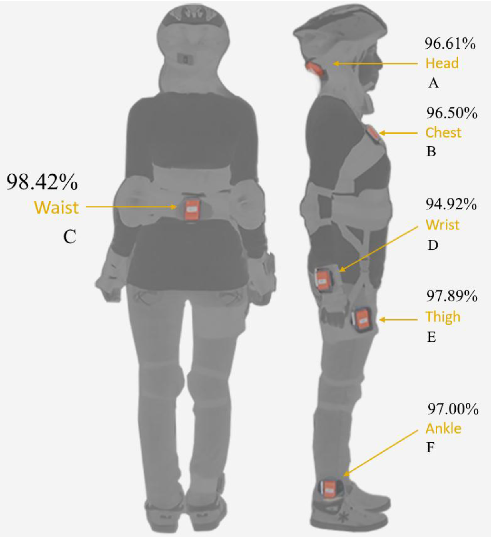
| Location of Sensor Unit | C (Waist) | E (Right-Thigh) | F (Right-Ankle) | A (Head) | B (Chest) | D (Right-Wrist) |
|---|---|---|---|---|---|---|
| Average Accuracy (%) | 98.42 | 97.89 | 97.00 | 96.61 | 96.50 | 94.92 |
| Algorithm | k-NN | BDM | SVM | LSM | DTW | ANN |
| Average Accuracy (%) | 99.21 | 97.77 | 97.49 | 96.64 | 95.64 | 94.58 |
| Individual Sensor Unit | C (Waist) | E (Right-Thigh) | B (Chest) | A (Head) | E (Right-Thigh) | C (Waist) |
| k-NN | k-NN | k-NN | k-NN | SVM | BDM | |
| Accuracy (%) | 99.87 | 99.61 | 99.60 | 99.50 | 99.27 | 99.24 |
| Sens. | Spec. | Vol. | Locat. | Comb. | Tests | Algorithms | Performances | |
|---|---|---|---|---|---|---|---|---|
| Bao [21] | 5× 2X A | ±10 g | 20 P 13 M 7 F | ankle arm thigh hip wrist | 20 | 20 20 ADL 0 fall | Decision Table Instant Learning Naïve Bayes Decision Tree | All Sensors 84.5% Acc thigh + wrist 80.73% Acc |
| Kangas [18] | 3× 3X A | ±12 g | 3 P 2 M 1 F | waist head wrist | 24 | 12 9 ADL 3 fall | Rule Based Alg. | 98% Head Se 97% Waist Se 71% Wrist Se |
| Li [19] | 2× 3X A 3X G | ±10 g ±500°/s | 3 P 3 M 0 F | chest thigh | 1 | 14 9 ADL 5 fall | Rule Based Alg. | chest + thigh 92% Acc 91% Se |
| Atallah [20] | 6× 3X G | ±3 g | 11 P 9 M 2 F | ankle knee waist wrist arm chest ear | 12 | 15 15 ADL | k-NN Bayesian Classifier | low level waist medium level chest, wrist high level arm, knee |
| Shi [22] | 21× 3X A 3X G 3X M | ±8 g ±2000°/s N/A | 13 P 12 M 1 F | thighs shanks feet u-arms f-arms hands waist neck head back | 14 | 25 12 ADL 13 fall | Decision Tree Algorithm | waist 97.79% Acc 95.5% Se 98.8% Sp |
| Özdemir [13] | 6× 3X A 3X G 3X M | ±16 g ±1200°/s ±1.5 G | 14 P 7 M 7 F | head chest waist wrist thigh knee | 378 | 36 16 ADL 20 fall | k-NN BDM SVM LSM DTW ANN | waist 99.87% Acc 99.96% Se 99.76% Sp |
© 2016 by the author; licensee MDPI, Basel, Switzerland. This article is an open access article distributed under the terms and conditions of the Creative Commons Attribution (CC-BY) license (http://creativecommons.org/licenses/by/4.0/).
Share and Cite
Özdemir, A.T. An Analysis on Sensor Locations of the Human Body for Wearable Fall Detection Devices: Principles and Practice. Sensors 2016, 16, 1161. https://doi.org/10.3390/s16081161
Özdemir AT. An Analysis on Sensor Locations of the Human Body for Wearable Fall Detection Devices: Principles and Practice. Sensors. 2016; 16(8):1161. https://doi.org/10.3390/s16081161
Chicago/Turabian StyleÖzdemir, Ahmet Turan. 2016. "An Analysis on Sensor Locations of the Human Body for Wearable Fall Detection Devices: Principles and Practice" Sensors 16, no. 8: 1161. https://doi.org/10.3390/s16081161
APA StyleÖzdemir, A. T. (2016). An Analysis on Sensor Locations of the Human Body for Wearable Fall Detection Devices: Principles and Practice. Sensors, 16(8), 1161. https://doi.org/10.3390/s16081161