
Strategic Decision-Making Learning from Label Distributions: An Approach for Facial Age Estimation

Abstract
:1. Introduction
- Difference of aging process: Different people have their own living environment, ethnic group, gender, lifestyle, social contact, health condition and even gene diversity, which all together determine the speed of aging.
- Shape or texture: Different forms of aging will emerge at different age levels. For example, from infancy to adolescence, the craniofacial growth (shape growth) is the main change. However, from adult period to old age, the craniofacial change decreases remarkably and skin transformation (texture change) would be the most prominent change.
- Data insufficiency: It takes great effort to search and collect old photos which were taken years ago. As a result, it is rather difficult for almost everyone to find one photo in each past year, let alone requiring the same shooting angle, lighting condition, resolution and background. In addition, only the past and present photos might be available, which means it is quite infrequent that a complete set of a person’s facial images with each age label can be gathered before his or her life ends. On the other hand, aging is a process which takes place moment by moment, so it is impossible to obtain multiple facial images for one person at the same time of different years. In fact, we only have a very limited number of aging datasets, especially that can cover the entire age range and are evenly distributed.
- Disturbance: Some females tend to show their younger faces, so final estimation results will be largely interfered with by using cosmetics and accessories.
2. Label Distribution Learning and Its Decision-Making Criterion
3. Strategic Decision-Making Label Distribution Learning (SDM-LDL) for Facial Age Estimation
3.1. Original Decision-Making Rule without Strategy
3.2. Strategic Decision-Making Algorithm (SDM-LDL) with Strategy 1
3.3. SDM-LDL with Strategy 2
3.4. SDM-LDL with Strategy 3
3.5. SDM-LDL with Strategy 4
3.6. SDM-LDL with Strategy 5
4. Experiments
4.1. Experimental Environment Settings
4.2. Methodology and Experimental Results
4.2.1. Gaussian-Like Distribution
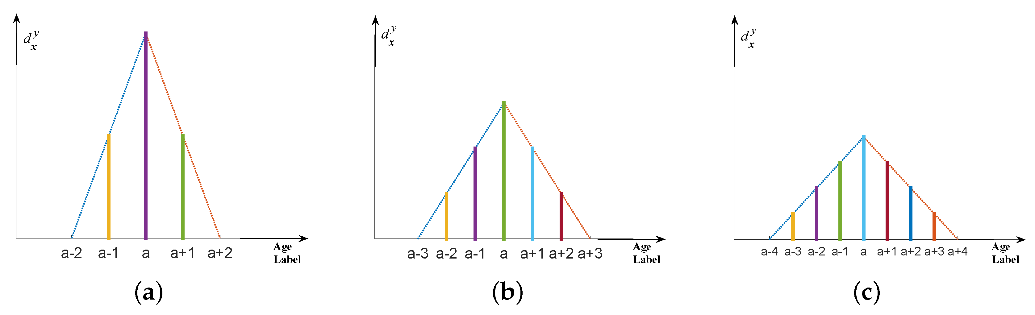
4.2.2. Triangle Distribution
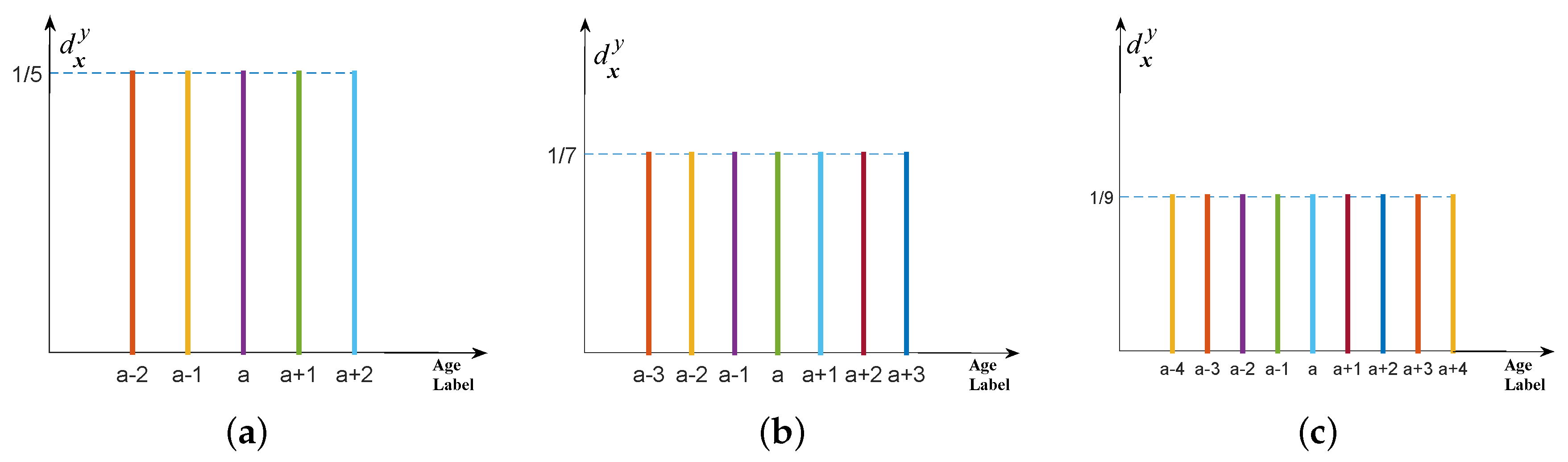
4.2.3. Multi-Label Distribution with Equal Description Degrees
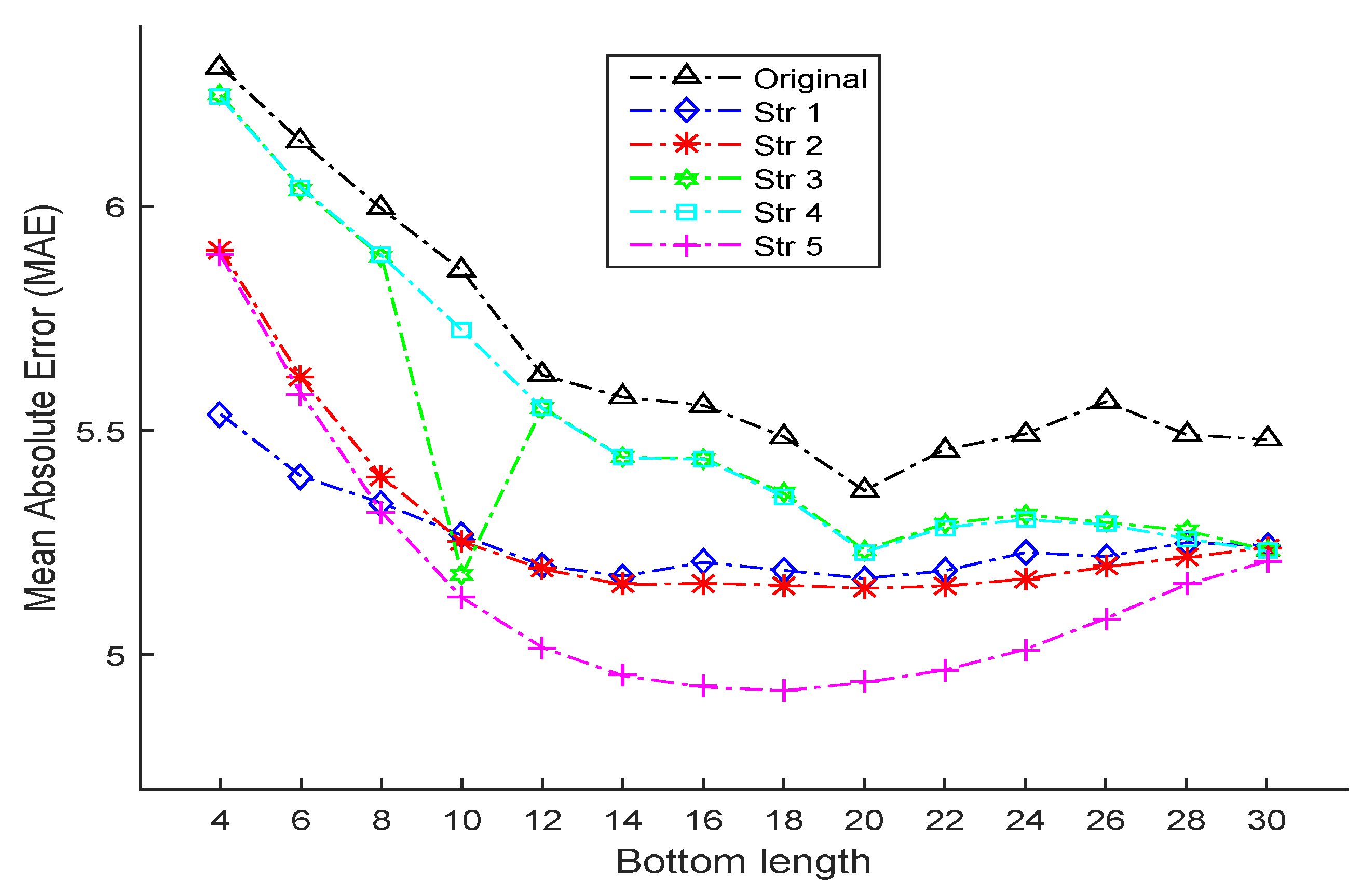
4.2.4. Overall comparison of the Proposed SDM-LDL Algorithms and Other Popular Algorithms
5. Conclusions
Acknowledgments
Author Contributions
Conflicts of Interest
References
- How-old.net. Microsoft. Available online: http://how-old.net (accessed on 25 June 2016).
- Electronic Customer Relationship Management (ECRM). Available online: http://en.wikipedia.org/wiki/ECRM (accessed on 25 June 2016).
- Kloeppel, J.E. Step Right up, Let the Computer Look at Your Face and Tell You Your Age. Available online: http://news.illinois.edu/news/08/0923age.html (accessed on 25 June 2016).
- Dix, A.; Finlay, J.; Abowd, G.D.; Beale, R. Human-Computer Interaction. Available online: http://fit.mta.edu.vn/files/DanhSach/__Human_computer_interaction.pdf (accessed on 25 June 2016).
- Guo, G.; Fu, Y.; Dyer, C.; Huang, T. Image-based human age estimation by manifold learning and locally adjusted robust regression. IEEE Trans. Image Process. 2008, 17, 1178–1188. [Google Scholar] [PubMed]
- Ramanathan, N.; Chellappa, R. Face verification across age progression. IEEE Trans. Image Process. 2006, 15, 3349–3361. [Google Scholar] [CrossRef] [PubMed]
- Albert, A.M.; Ricanek, K.; Pattersonb, E. A review of the literature on the aging adult skull and face: Implications for forensic science research and applications. Forensic Sci. Int. 2007, 172, 1–9. [Google Scholar] [CrossRef] [PubMed]
- Weng, R.; Lu, J.; Yang, G.; Tan, Y. Multi-feature ordinal ranking for facial age estimation. In Proceedings of the IEEE International Conference and Workshops on Automatic Face and Gesture Recognition, Shanghai, China, 22–26 April 2013; pp. 1–6.
- Wang, C.; Su, Y.; Hsu, C.; Lin, C.; Liao, H. Bayesian age estimation on face images. In Proceedings of the IEEE Conf. on Multimedia and Expo, New York, NY, USA, 28 June–3 July 2009; pp. 282–285.
- Geng, X.; Zhou, Z.; Smith-Miles, K. Automatic age estimation based on facial aging patterns. IEEE Trans. Pattern Anal. Mach. Intell. 2007, 29, 2234–2240. [Google Scholar] [CrossRef] [PubMed]
- Lanitis, A.; Draganova, C.; Christodoulou, C. Comparing different classifiers for automatic age estimation. IEEE Trans. Syst. Man Cybernet. Part B 2004, 34, 621–628. [Google Scholar] [CrossRef]
- Yang, Z.; Ai, H. Demographic classification with local binary patterns. In Proceedings of the International Conference on Biometrics, Seoul, Korea, 27–29 August 2007; pp. 464–473.
- Fu, Y.; Huang, T. Human age estimation with regression on discriminative aging manifold. IEEE Trans. Multimedia 2008, 10, 578–584. [Google Scholar] [CrossRef]
- Zhang, Y.; Yeung, D. Multi-task warped Gaussian process for personalized age estimation. In Proceedings of the IEEE Conference on Computer Vision and Pattern Recognition, San Francisco, CA, USA, 13–18 June 2010; pp. 2622–2629.
- Ni, B.; Song, Z.; Yan, S. Web image mining towards universal age estimator. In Proceedings of the ACM International Conference on Multimedia, Beijing, China, 19–24 October 2009; pp. 85–94.
- Xiao, B.; Yang, X.; Zha, H.; Xu, Y.; Huang, T. Metric Learning for Regression Problems and Human Age Estimation. In Advances in Multimedia Information Processing—PCM 2009; Springer: Berlin, Germany, 2009; Volume 5879, pp. 88–99. [Google Scholar]
- Guo, G.; Fu, Y.; Huang, T.; Dyer, C. Locally adjusted robust regression for human age estimation. In Proceedings of the IEEE Workshop on Applications of Computer Vision, Copper Mountain, CO, USA, 7–9 January 2008; pp. 1–6.
- Chang, K.; Chen, C.; Hung, Y. Ordinal hyperplanes ranker with cost sensitivities for age estimation. In Proceedings of the IEEE Conference on Computer Vision and Pattern Recognition, Providence, RI, USA, 20–25 June 2011; pp. 585–592.
- Yan, S.; Wang, H.; Huang, T.; Yang, Q. Ranking with uncertain labels. In Proceedings of the IEEE Conference on Multimedia and Expo, Beijing, China, 2–5 July 2007; pp. 96–99.
- Chao, W.L.; Liu, J.Z.; Ding, J.J. Facial age estimation based on label-sensitive learning and age-oriented regression. Pattern Recognit. 2013, 46, 628–641. [Google Scholar] [CrossRef]
- Geng, X.; Yin, C.; Zhou, Z.H. Facial age estimation by learning from label distributions. IEEE Trans. Pattern Anal. Mach. Intell. 2013, 35, 2401–2412. [Google Scholar] [CrossRef] [PubMed]
- Geng, X.; Ji, R. Label distribution learning. In Proceedings of the 13th International Conference on Data Mining Workshops (ICDMW), Dallas, TX, USA, 7–10 December 2013; pp. 377–383.
- The FG-NET Aging Database. Available online: http://www.fgnet.rsunit.com/ (accessed on 5 September 2010).
- Berger, A.L.; Pietra, S.D.; Pietra, V.J.D. A maximum entropy approach to natural language processing. Comput. Linguist. 1996, 22, 39–71. [Google Scholar]
- Cootes, T.F.; Edwards, G.J.; Taylor, C.J. Active appearance models. IEEE Trans. Pattern Anal. Mach. Intell. 2001, 23, 681–685. [Google Scholar] [CrossRef]
- Guo, G.; Mu, G.; Fu, Y.; Huang, T. Human age estimation using bio-inspired features. In Proceedings of the IEEE Conference on Computer Vision and Pattern Recognition, Miami, FL, USA, 20–25 June 2009; pp. 112–119.
- Yang, P.; Zhong, L.; Metaxas, D. Ranking model for facial age estimation. In Proceedings of the International Conference on Pattern Recognition, Istanbul, Turkey, 23–26 August 2010; pp. 3404–3407.
- Yan, S.; Wang, H.; Tang, X.; Huang, T. Learning auto-structured regressor from uncertain nonnegative labels. In Proceedings of the International Conference on Computer Vision, Rio de Janeiro, Brazil, 14–21 October 2007; pp. 1–8.
- Liang, Y.; Wang, X.; Zhang, L.; Wang, Z. A hierarchical framework for facial age estimation. Math. Probl. Eng. 2014. [Google Scholar] [CrossRef]
- Ylioinas, J.; Hadid, A.; Hong, X.; Pietikainen, M. Age estimation using local binary pattern kernel density estimate. In Proceedings of the 17th International Conferenceon Image Analysis and Processing, Naples, Italy, 9–13 September 2013; pp. 141–150.
- Gunay, A.; Nabiyev, V.V. Age estimation based on local radon features of facial images. In Computer and Information Sciences III; Springer: Berlin, Germany, 2013; pp. 183–190. [Google Scholar]
- Chen, K.; Gong, S.; Xiang, T.; Loy, C.C. Cumulative attribute space for age and crowd density estimation. In Proceedings of the IEEE Conference on Computer Vision and Pattern Recognition, Portland, OR, USA, 23–28 June 2013; pp. 2467–2474.
- Wu, T.; Turaga, P.; Chellappa, R. Age estimation and face verification across aging using landmarks. IEEE Trans. Inf. Forensics Secur. 2012, 7, 1780–1788. [Google Scholar] [CrossRef]
- Zhang, L.; Wang, X.; Liang, Y.; Xie, L. A new method for age estimation from facial images by hierarchical model. In Proceedings of the International Conference on Innovative Computing and Cloud Computing, Wuhan, China, 1–2 December 2013; p. 88.
- Thukral, P.; Mitra, K.; Chellappa, R. A hierarchical approach for human age estimation. In Proceedings of the IEEE Internationl Conference on Acoustics, Speech and Signal Processing, Kyoto, Japan, 25–30 March 2012; pp. 1529–1532.
- Xiao, B.; Yang, X.; Xu, Y.; Zha, H. Learning distance metric for regression by semidefinite programming with application to human age estimation. In Proceedings of the ACM Internationl Conference on Multimedia, Beijing, China, 19–24 October 2009; pp. 451–460.
- Yan, S.; Wang, H.; Fu, Y.; Yan, J.; Tang, X.; Huang, T.S. Synchronized submanifold embedding for person-independent pose estimation and beyond. IEEE Trans. Image Process. 2009, 18, 202–210. [Google Scholar] [PubMed]


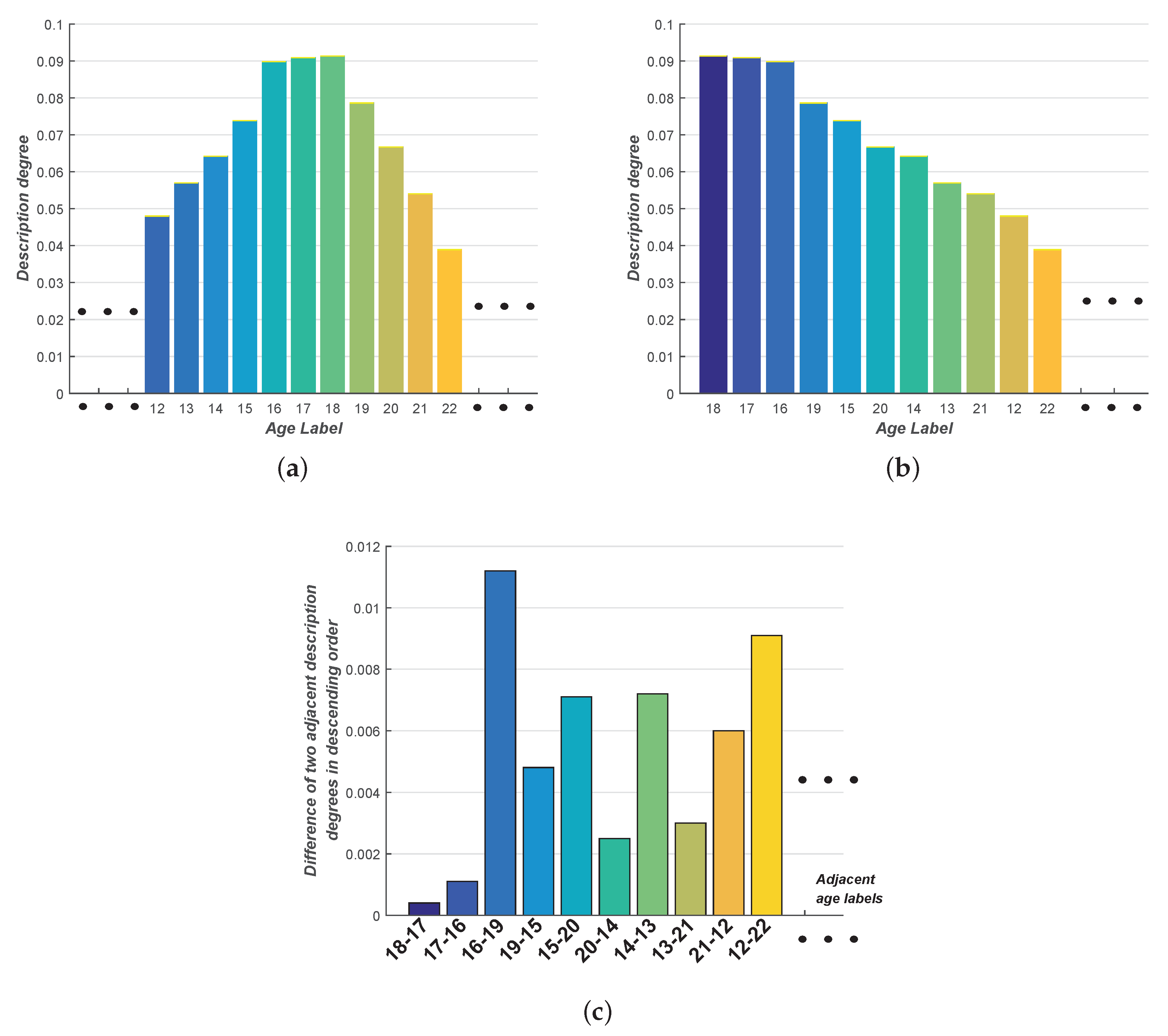
| Age Label | 0 | 1 | 2 | ... | 12 | 13 | 14 | 15 | 16 |
|---|---|---|---|---|---|---|---|---|---|
| Description degree | 0.0010 | 0.0017 | 0.0026 | ... | 0.0480 | 0.0570 | 0.0642 | 0.0738 | 0.0898 |
| Age Label | 17 | 18 | 19 | 20 | 21 | 22 | ... | 68 | 69 |
| Description degree | 0.0909 | 0.0913 | 0.0786 | 0.0667 | 0.0540 | 0.0389 | ... | 1.0667 | 2.7528 |
| Age Label | 18 | 17 | 16 | 19 | 15 | 20 | 14 | 13 | 21 | 12 | 22 | ... |
|---|---|---|---|---|---|---|---|---|---|---|---|---|
| Description degree (descending order) | 0.0913 | 0.0909 | 0.0898 | 0.0786 | 0.0738 | 0.0667 | 0.0642 | 0.0570 | 0.0540 | 0.0480 | 0.0389 | ... |
| Difference () | 4e-04 | 0.0011 | 0.0112 | 0.0048 | 0.0071 | 0.0025 | 0.0072 | 0.0030 | 0.0060 | 0.0091 | ... | ... |
| Deviation from Authentic Age (Absolute Value) | |
|---|---|
| Original LDL | 2.0000 |
| SDM-LDL (Str 1) | 0.5000 |
| SDM-LDL (Str 2) | 0.6732 |
| SDM-LDL (Str 3) | 1.0000 |
| SDM-LDL (Str 4) | 1.0055 |
| SDM-LDL (Str 5) | 0.2586 |
| Range of Age | FG-NET | |
|---|---|---|
| #img. | % | |
| 0–9 | 371 | 37.03 |
| 10–19 | 339 | 33.83 |
| 20–29 | 144 | 14.37 |
| 30–39 | 79 | 7.88 |
| 40–49 | 46 | 4.59 |
| 50–59 | 15 | 1.50 |
| 60–69 | 8 | 0.80 |
| Total | 1002 | 100 |
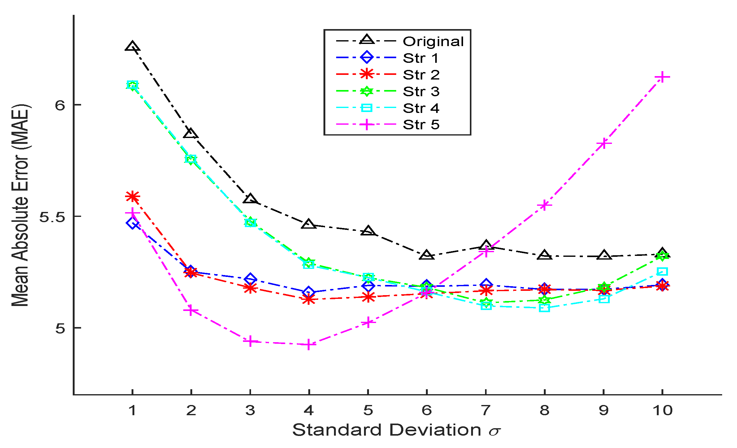
| σ | 1 | 2 | 3 | 4 | 5 |
| MAE (Ori) | 6.261 | 5.868 | 5.573 | 5.462 | 5.431 |
| MAE (Str 1) | 5.471 (N = 8) | 5.251 (N = 9) | 5.219 (N = 9) | 5.159 (N = 9) | 5.190 (N = 9) |
| MAE (Str 2) | 5.588 (N = 10) | 5.246 (N = 10) | 5.180 (N = 10) | 5.127 (N = 10) | 5.139 (N = 10) |
| MAE (Str 3) | 6.084 | 5.753 | 5.478 | 5.290 | 5.225 |
| MAE (Str 4) | 6.088 | 5.760 | 5.473 | 5.280 | 5.226 |
| MAE (Str 5) | 5.513 | 5.080 | 4.938 | 4.920 | 5.023 |
| σ | 6 | 7 | 8 | 9 | 10 |
| MAE (Ori) | 5.321 | 5.366 | 5.322 | 5.320 | 5.330 |
| MAE (Str 1) | 5.186 (N = 9) | 5.192 (N = 9) | 5.172 (N = 5) | 5.173 (N = 7) | 5.192 (N = 7) |
| MAE (Str 2) | 5.153 (N = 9) | 5.166 (N = 9) | 5.171 (N = 5) | 5.168 (N = 7) | 5.187 (N = 7) |
| MAE (Str 3) | 5.181 | 5.112 | 5.125 | 5.184 | 5.321 |
| MAE (Str 4) | 5.161 | 5.098 | 5.089 | 5.130 | 5.252 |
| MAE (Str 5) | 5.157 | 5.344 | 5.550 | 5.828 | 6.126 |
| σ | 1 | 2 | 3 | 4 | 5 | 6 | 7 | 8 | 9 | 10 | |
|---|---|---|---|---|---|---|---|---|---|---|---|
| MAE (Str 1) | N = 2 | 5.978 | 5.725 | 5.500 | 5.384 | 5.414 | 5.286 | 5.339 | 5.264 | 5.279 | 5.278 |
| N = 3 | 5.741 | 5.592 | 5.397 | 5.327 | 5.358 | 5.275 | 5.303 | 5.221 | 5.237 | 5.226 | |
| N = 4 | 5.569 | 5.528 | 5.362 | 5.301 | 5.339 | 5.258 | 5.306 | 5.205 | 5.222 | 5.229 | |
| N = 5 | 5.508 | 5.401 | 5.335 | 5.252 | 5.263 | 5.233 | 5.248 | 5.172 | 5.193 | 5.201 | |
| N = 6 | 5.484 | 5.362 | 5.286 | 5.226 | 5.278 | 5.206 | 5.246 | 5.196 | 5.196 | 5.208 | |
| N = 7 | 5.511 | 5.307 | 5.233 | 5.195 | 5.219 | 5.189 | 5.209 | 5.181 | 5.173 | 5.192 | |
| N = 8 | 5.471 | 5.285 | 5.245 | 5.200 | 5.224 | 5.199 | 5.211 | 5.213 | 5.188 | 5.254 | |
| N = 9 | 5.531 | 5.251 | 5.219 | 5.159 | 5.190 | 5.186 | 5.192 | 5.207 | 5.189 | 5.223 | |
| N = 10 | 5.627 | 5.263 | 5.241 | 5.196 | 5.205 | 5.241 | 5.245 | 5.260 | 5.226 | 5.305 | |
| MAE (Str 2) | N = 2 | 6.025 | 5.741 | 5.501 | 5.385 | 5.413 | 5.287 | 5.339 | 5.265 | 5.280 | 5.278 |
| N = 3 | 5.870 | 5.623 | 5.408 | 5.328 | 5.359 | 5.274 | 5.303 | 5.222 | 5.238 | 5.228 | |
| N = 4 | 5.782 | 5.568 | 5.373 | 5.300 | 5.337 | 5.257 | 5.303 | 5.203 | 5.221 | 5.229 | |
| N = 5 | 5.724 | 5.473 | 5.343 | 5.256 | 5.266 | 5.233 | 5.247 | 5.171 | 5.191 | 5.200 | |
| N = 6 | 5.689 | 5.422 | 5.296 | 5.223 | 5.270 | 5.199 | 5.238 | 5.191 | 5.191 | 5.204 | |
| N = 7 | 5.647 | 5.367 | 5.251 | 5.194 | 5.215 | 5.181 | 5.201 | 5.174 | 5.168 | 5.187 | |
| N = 8 | 5.621 | 5.323 | 5.224 | 5.180 | 5.200 | 5.175 | 5.192 | 5.195 | 5.175 | 5.240 | |
| N = 9 | 5.599 | 5.284 | 5.203 | 5.143 | 5.161 | 5.153 | 5.166 | 5.185 | 5.171 | 5.208 | |
| N = 10 | 5.588 | 5.246 | 5.180 | 5.127 | 5.139 | 5.170 | 5.189 | 5.216 | 5.193 | 5.273 | |
| Bottom Length | 4 | 6 | 8 | 10 | 12 | 14 | 16 |
| MAE (Ori) | 6.310 | 6.144 | 5.994 | 5.856 | 5.623 | 5.574 | 5.556 |
| MAE (Str 1) | 5.536 (N = 7) | 5.398 (N = 7) | 5.338 (N = 8) | 5.266 (N = 7) | 5.199 (N = 9) | 5.175 (N = 10) | 5.206 (N = 10) |
| MAE (Str 2) | 5.903 (N = 10) | 5.617 (N = 10) | 5.397 (N = 10) | 5.252 (N = 10) | 5.191 (N = 10) | 5.156 (N = 10) | 5.159 (N = 10) |
| MAE (Str 3) | 6.247 | 6.038 | 5.887 | 5.178 | 5.551 | 5.440 | 5.438 |
| MAE (Str 4) | 6.242 | 6.041 | 5.890 | 5.723 | 5.549 | 5.439 | 5.436 |
| MAE (Str 5) | 5.890 | 5.582 | 5.318 | 5.127 | 5.016 | 4.953 | 4.928 |
| Bottom Length | 18 | 20 | 22 | 24 | 26 | 28 | 30 |
| MAE (Ori) | 5.486 | 5.366 | 5.458 | 5.492 | 5.564 | 5.491 | 5.479 |
| MAE (Str 1) | 5.188 (N = 9) | 5.170 (N = 9) | 5.187 (N = 9) | 5.228 (N = 7) | 5.219 (N = 9) | 5.250 (N = 9) | 5.244 (N = 7) |
| MAE (Str 2) | 5.155 (N = 10) | 5.148 (N = 9) | 5.153 (N = 10) | 5.169 (N = 10) | 5.196 (N = 10) | 5.217 (N = 9) | 5.239 (N = 9) |
| MAE (Str 3) | 5.360 | 5.234 | 5.292 | 5.312 | 5.295 | 5.277 | 5.234 |
| MAE (Str 4) | 5.353 | 5.229 | 5.284 | 5.301 | 5.290 | 5.259 | 5.231 |
| MAE (Str 5) | 4.925 | 4.938 | 4.966 | 5.012 | 5.081 | 5.156 | 5.208 |
| Bottom Length | 4 | 6 | 8 | 10 | 12 | 14 | 16 | 18 | 20 | 22 | 24 | 26 | 28 | 30 | |
|---|---|---|---|---|---|---|---|---|---|---|---|---|---|---|---|
| MAE (Str 1) | N = 2 | 5.861 | 5.802 | 5.833 | 5.640 | 5.549 | 5.486 | 5.477 | 5.453 | 5.373 | 5.445 | 5.438 | 5.444 | 5.414 | 5.436 |
| N = 3 | 5.656 | 5.646 | 5.692 | 5.524 | 5.456 | 5.402 | 5.402 | 5.385 | 5.358 | 5.395 | 5.398 | 5.409 | 5.364 | 5.403 | |
| N = 4 | 5.640 | 5.578 | 5.523 | 5.449 | 5.421 | 5.309 | 5.384 | 5.374 | 5.326 | 5.375 | 5.351 | 5.382 | 5.365 | 5.369 | |
| N = 5 | 5.553 | 5.463 | 5.444 | 5.338 | 5.324 | 5.302 | 5.300 | 5.293 | 5.247 | 5.289 | 5.276 | 5.304 | 5.324 | 5.326 | |
| N = 6 | 5.542 | 5.423 | 5.388 | 5.323 | 5.260 | 5.269 | 5.309 | 5.261 | 5.258 | 5.250 | 5.245 | 5.305 | 5.314 | 5.313 | |
| N = 7 | 5.536 | 5.398 | 5.341 | 5.266 | 5.217 | 5.229 | 5.258 | 5.248 | 5.207 | 5.199 | 5.228 | 5.250 | 5.261 | 5.244 | |
| N = 8 | 5.673 | 5.438 | 5.338 | 5.276 | 5.221 | 5.208 | 5.234 | 5.227 | 5.201 | 5.209 | 5.230 | 5.258 | 5.258 | 5.259 | |
| N = 9 | 5.774 | 5.437 | 5.344 | 5.275 | 5.199 | 5.181 | 5.237 | 5.188 | 5.170 | 5.187 | 5.234 | 5.219 | 5.250 | 5.268 | |
| N = 10 | 5.845 | 5.485 | 5.386 | 5.307 | 5.231 | 5.175 | 5.206 | 5.211 | 5.222 | 5.215 | 5.235 | 5.259 | 5.314 | 5.300 | |
| MAE (Str 2) | N = 2 | 6.071 | 5.888 | 5.838 | 5.663 | 5.554 | 5.485 | 5.483 | 5.451 | 5.371 | 5.443 | 5.439 | 5.444 | 5.416 | 5.434 |
| N = 3 | 5.984 | 5.793 | 5.729 | 5.567 | 5.481 | 5.417 | 5.414 | 5.388 | 5.357 | 5.396 | 5.398 | 5.410 | 5.367 | 5.402 | |
| N = 4 | 5.964 | 5.743 | 5.634 | 5.496 | 5.456 | 5.339 | 5.391 | 5.374 | 5.319 | 5.375 | 5.353 | 5.383 | 5.366 | 5.368 | |
| N = 5 | 5.941 | 5.706 | 5.562 | 5.431 | 5.384 | 5.332 | 5.321 | 5.301 | 5.244 | 5.296 | 5.283 | 5.312 | 5.327 | 5.327 | |
| N = 6 | 5.929 | 5.673 | 5.496 | 5.370 | 5.330 | 5.294 | 5.313 | 5.265 | 5.246 | 5.251 | 5.244 | 5.301 | 5.308 | 5.309 | |
| N = 7 | 5.919 | 5.648 | 5.457 | 5.334 | 5.289 | 5.263 | 5.270 | 5.250 | 5.207 | 5.202 | 5.223 | 5.247 | 5.256 | 5.242 | |
| N = 8 | 5.912 | 5.640 | 5.438 | 5.309 | 5.252 | 5.229 | 5.229 | 5.218 | 5.184 | 5.194 | 5.207 | 5.236 | 5.237 | 5.241 | |
| N = 9 | 5.908 | 5.629 | 5.416 | 5.280 | 5.221 | 5.193 | 5.208 | 5.176 | 5.148 | 5.166 | 5.199 | 5.199 | 5.217 | 5.239 | |
| N = 10 | 5.903 | 5.617 | 5.397 | 5.252 | 5.191 | 5.156 | 5.159 | 5.155 | 5.151 | 5.153 | 5.169 | 5.196 | 5.242 | 5.243 | |
| Number of Labels | 3 | 5 | 7 | 9 | 11 | 13 | 15 |
|---|---|---|---|---|---|---|---|
| MAE (Ori) | 6.312 | 5.998 | 5.830 | 5.700 | 5.698 | 5.732 | 5.690 |
| MAE (Str 1) | 5.541 (N = 5) | 5.343 (N = 8) | 5.219 (N = 7) | 5.175 (N = 8) | 5.169 (N = 7) | 5.137 (N = 9) | 5.139 (N = 9) |
| MAE (Str 2) | 5.979 (N = 10) | 5.638 (N = 10) | 5.312 (N = 10) | 5.219 (N = 10) | 5.145 (N = 10) | 5.127 (N = 10) | 5.132 (N = 10) |
| MAE (Str 3) | 6.242 | 5.952 | 5.742 | 5.645 | 5.540 | 5.537 | 5.530 |
| MAE (Str 4) | 6.245 | 5.957 | 5.737 | 5.650 | 5.542 | 5.548 | 5.528 |
| MAE (Str 5) | 5.974 | 5.626 | 5.263 | 5.143 | 5.017 | 5.002 | 5.009 |
| Gaussian-Like | Triangle | Multi-Label with Equal Description Degrees | |
|---|---|---|---|
| MAE (Ori) | 5.320 | 5.366 | 5.69 |
| MAE (Str 1) | 5.159 | 5.170 | 5.137 |
| MAE (Str 2) | 5.127 | 5.148 | 5.127 |
| MAE (Str 3) | 5.112 | 5.178 | 5.530 |
| MAE (Str 4) | 5.089 | 5.229 | 5.528 |
| MAE (Str 5) | 4.920 | 4.925 | 5.002 |
| Method | MAE |
|---|---|
| SDM-LDL(Str 1) | 5.137 |
| SDM-LDL(Str 2) | 5.127 |
| SDM-LDL(Str 3) | 5.112 |
| SDM-LDL(Str 4) | 5.089 |
| SDM-LDL(Str 5) | 4.920 |
| Original LDL | 5.32 |
| Hierarchical Framework [29] | 4.97 |
| LBP Kernel Density Estimate [30] | 5.09 |
| Local radon Features [31] | 6.18 |
| Cumulative Attribute SVR [32] | 4.67 |
| Grassmann Manifold [33] | 5.89 |
| Hierarchical Model [34] | 4.89 |
| Ordinal Hyperplanes Ranker (OHRank) [18] | 6.27 |
| Shape-based age estimation [35] | 6.2 |
| Regression using a learned distance metric [36] | 5.04 |
| Bio-inspired Features [26] | 4.77 |
| Synchronized Submanifold Embedding [37] | 5.21 |
| Manifold Learning and Locally Adjusted Robust Regressor [5] | 5.07 |
| Facial Aging Patterns (AGES) [10] | 6.77 |
| SVM | 7.25 |
| kNN | 8.24 |
© 2016 by the authors; licensee MDPI, Basel, Switzerland. This article is an open access article distributed under the terms and conditions of the Creative Commons Attribution (CC-BY) license (http://creativecommons.org/licenses/by/4.0/).
Share and Cite
Zhao, W.; Wang, H. Strategic Decision-Making Learning from Label Distributions: An Approach for Facial Age Estimation. Sensors 2016, 16, 994. https://doi.org/10.3390/s16070994
Zhao W, Wang H. Strategic Decision-Making Learning from Label Distributions: An Approach for Facial Age Estimation. Sensors. 2016; 16(7):994. https://doi.org/10.3390/s16070994
Chicago/Turabian StyleZhao, Wei, and Han Wang. 2016. "Strategic Decision-Making Learning from Label Distributions: An Approach for Facial Age Estimation" Sensors 16, no. 7: 994. https://doi.org/10.3390/s16070994
APA StyleZhao, W., & Wang, H. (2016). Strategic Decision-Making Learning from Label Distributions: An Approach for Facial Age Estimation. Sensors, 16(7), 994. https://doi.org/10.3390/s16070994