
A Depth-Adjustment Deployment Algorithm Based on Two-Dimensional Convex Hull and Spanning Tree for Underwater Wireless Sensor Networks

Abstract
:1. Introduction
- (1)
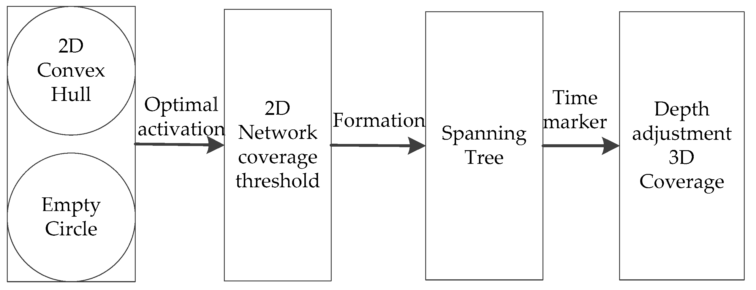
- The geometric characteristics of the 2D convex hull and empty circle is used to minimize the 2D plane network coverage overlaps, with a minimum number of activated nodes to meet the requirement of the first layer of the network deployment.
- (2)
- The activation scheduling mechanism is adopted to reduce the energy consumption of communication between nodes.
- (3)
- The adjustable communication radius model is established to ensure that all active nodes have full network connectivity in the first layer. In addition, in the process of depth adjustment, the communication connection is guaranteed between the parent and its child nodes in real time.
- (4)
- Depth adjustment is based on the time marker, adjacent time marker neighbor nodes set is dominated by its parent node, and it is a perfect approach to balance the density of node deployment. When the set is empty, the neighbor nodes intersect to execute depth-adjustment assignment, ensuring that the network deployment performance of near water bottom is relatively good and that network operation is more reliable. Overall, our work optimizes network coverage rate under the premise of full network connectivity, reducing the energy consumption of communication.
2. Related Works
3. Network Models and Related Definitions
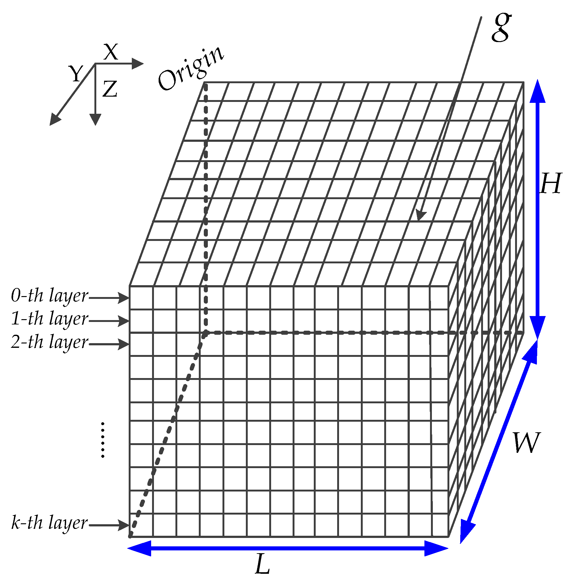
3.1. Network Models
3.1.1. Network System Model
- (1)
- The node has no ability to perceive global coordinate information in 3D network space, and merely the node perceives own depth information.
- (2)
- Each node has a unique identity ID.
- (3)
- The boundary effect is negligible because the node communication radius Rc and sensing radius Rs are significantly smaller than the length L, width W, or height H of the 3D monitoring space.
- (4)
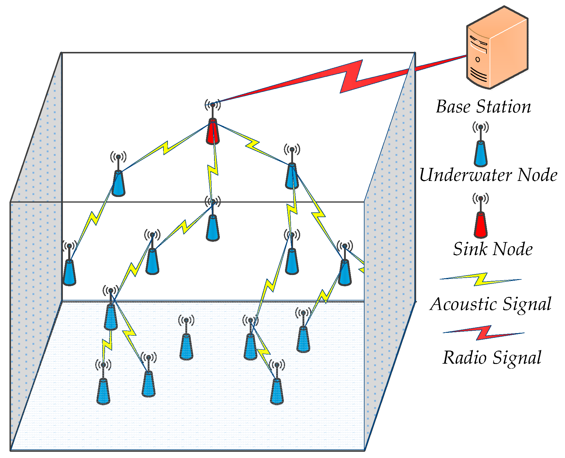
- All nodes use a uniform acoustic signal to transmit and receive information, and the sink node transmits the information to the base station by radio signal.
- (5)
- All nodes are identical and have the same initial energy Einit, sensing radius Rs, and the initial communication radius Rcinit. Moreover, the energy consumption of the sink node is negligible.
3.1.2. Node Perception Model
3.1.3. Adjustable Communication Radius Model
3.1.4. Node Energy Consumption Model
3.2. Related Definitions
3.2.1. Network Coverage Rate
3.2.2. Network Connectivity Rate
3.2.3. Network Reliability
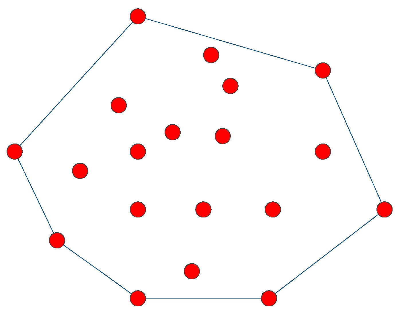
3.2.4. Two-Dimensional Convex Hull
3.2.5. Empty Circle
4. Problem Analysis and Algorithm Description
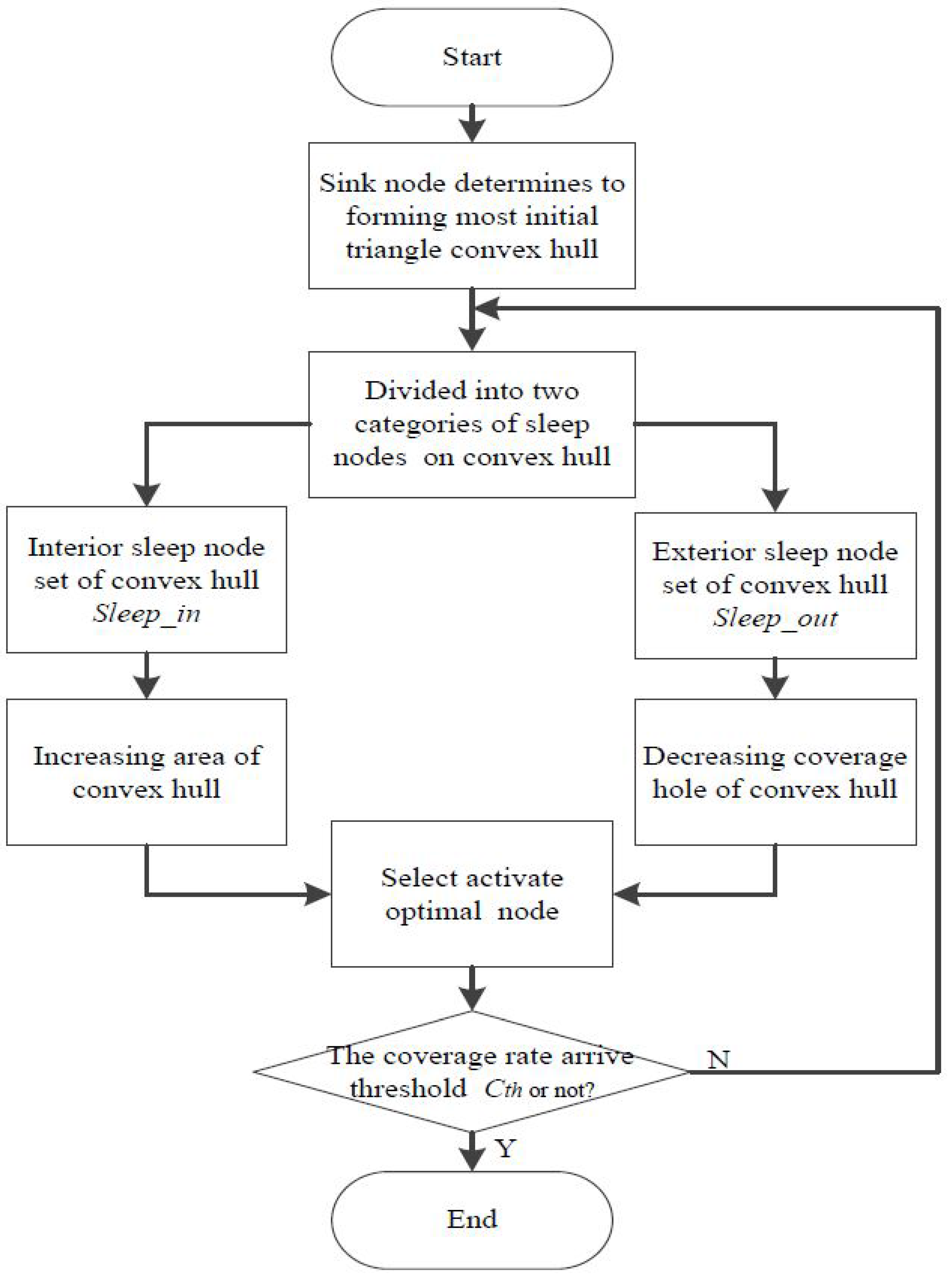
4.1. Problem Analysis
4.2. Algorithm Description
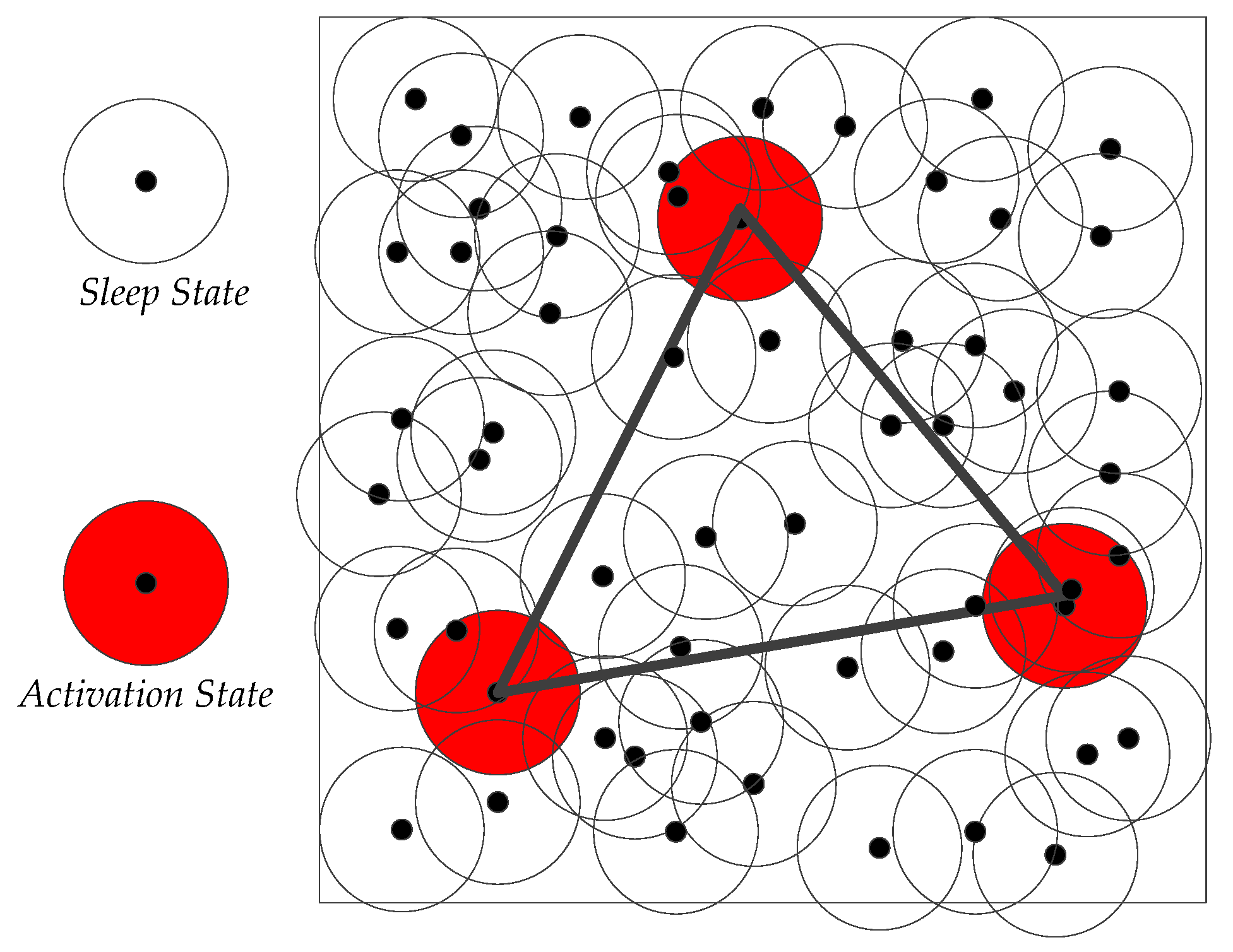
4.2.1. Optimal Activation Strategy Based on 2D Convex Hull
4.2.2. Formation Process of 2D Convex Hull Spanning Tree
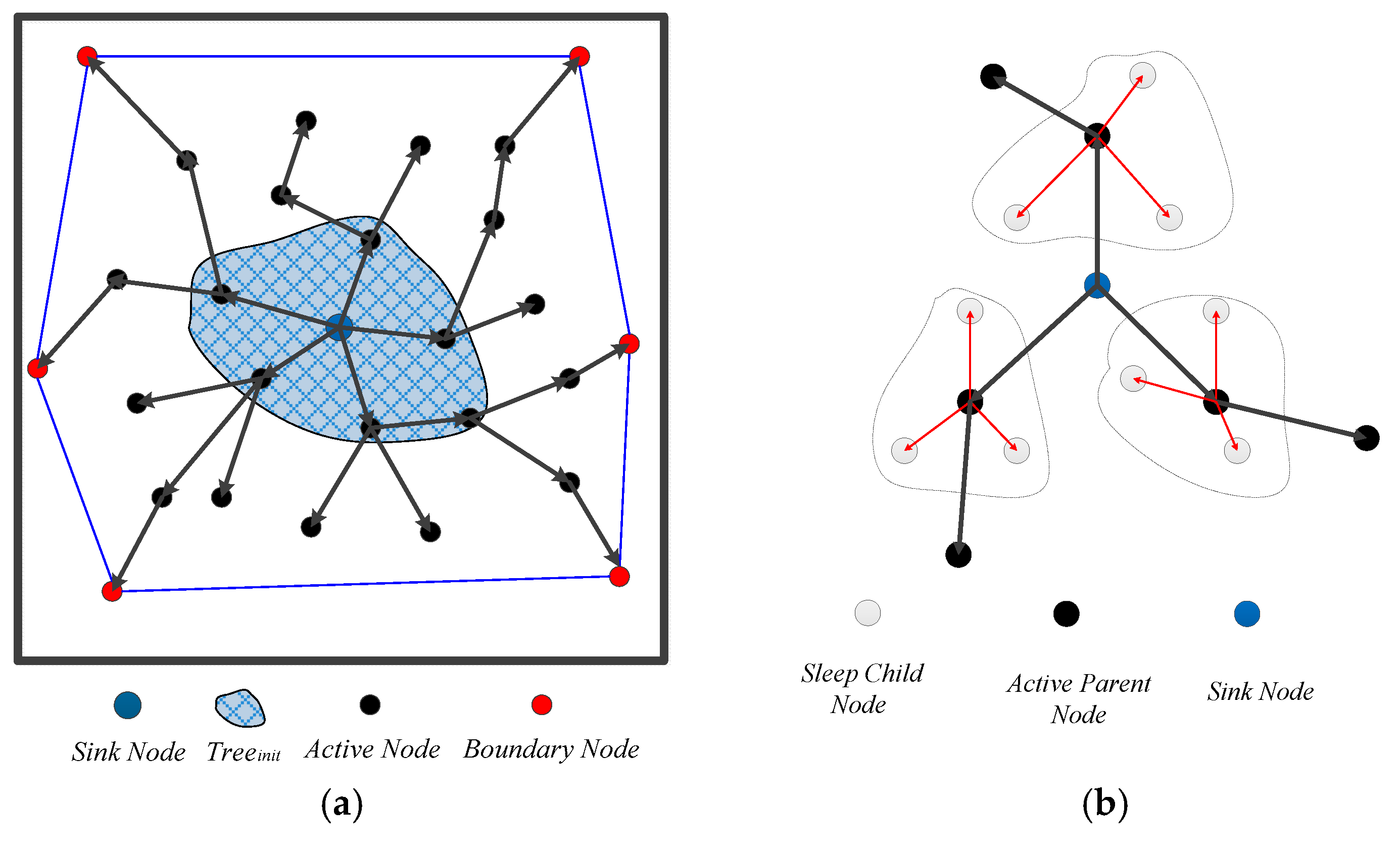
- (1)
- The tree root node r and set of active neighbor nodes Nei_A form an initial spanning tree Treeinit as shown in Figure 7a. The iterative strategy is adopted to produce a next spanning tree generation according to the size of IDA, until all active nodes of the 2D convex hull form a complete initial spanning forest Forestinit. Whether a parent node and its child nodes on spanning forest Forestinit are able to communicate, if not, by Section 3.1.3, the communication radius is incremented until the parent node is connected to its child nodes so that the initial spanning forest Forestinit can maintain full network connectivity.
- (2)
- The time marker Tmark of root node r is initialized to 0, and the next generation of child nodes’ time marker increments by 1, until all active nodes of the initial spanning forest Forestinit are marked to the T level (i.e., all of CH_node are marked by the r node). The Tmark of the same subtree parent node set {fji} (j denotes IDA; i denotes Tmark) is recorded.
- (3)
- The active node inside the 2D convex hull Sa_in (IDA) acts as the parent of its neighboring sleeping nodes. Building a small spanning tree of individual nodes on Forestinit, we define a small spanning tree consisting of hybrid construction where the parent is the active node and the child is the sleeping node, as shown in Figure 7b.
- (4)
- To achieve the 3D global network coverage, the algorithm needs to deploy neighboring sleeping nodes Nei(fji) distributed at different depths and calculate the depth adjustment of the set of subtree parent nodes {fji} for their child sleeping nodes.
4.2.3. Depth-Adjustment Strategy Based on Time Markers
- (1)
- The set of neighbor nodes {Nei (f*i)} under the same network hierarchy (the same time marker i) are recorded, and then whether two sets of neighboring sleeping nodes intersect under the neighbor time marker and same path of tree is determined. If an intersection exists, then it is NeigInteri+1 between time marker i and i + 1; otherwise, an empty set is recorded to NeigInterii+1.
- (2)
- Time marker Tmark is initialized to 1, that is, Tmark = 1. The active node fji inside the convex hull sends an awaken message AWAKEN_MES to the set of non-intersecting neighboring nodes Nei(fji) − NeigInterii+1 and activates them. Node fji builds a horizontal distance state table Horizontal_Dis(fji, Nei(fji) − NeigInteri i+1) according to the distance between the child elements of Nei(fji) − NeigInterii+1 and their parent nodes fji from small to large. Thereafter, a node fimin is selected with a minimum value min(Hor_Dis) on the state table as a depth-adjustment standard. Therefore, the drop-distance ver_dis of non-intersecting neighbor nodes set Neig(fji) − NeigInterii+1 is calculated by Equation (14):where Rcmax denotes the maximum communication radius after adjusted and can maintain connectivity between parent node fji and its child node.
- (3)
- Furthermore, node fji submits a permission to its child node fimin and makes it as a parent node of the set of neighbor nodes Nei(fji) − NeigInterii+1. Thereafter, fimin is still used its time marker of parent node fji. According to the size of the order of IDA to all neighbor nodes on the same time marker adopting the depth-adjustment method of step (2) to adjust the depth of the other child nodes of Nei(fji) − NeigInterii+1, node fji sends a sleep message SLEEP_MES to its neighbor node and converts them to sleep state. Thereafter, Tmark = Tmark + 1, and the above depth-adjustment process is repeated for fji until all CH_node is marked, achieving a layer depth adjustment.
- (4)
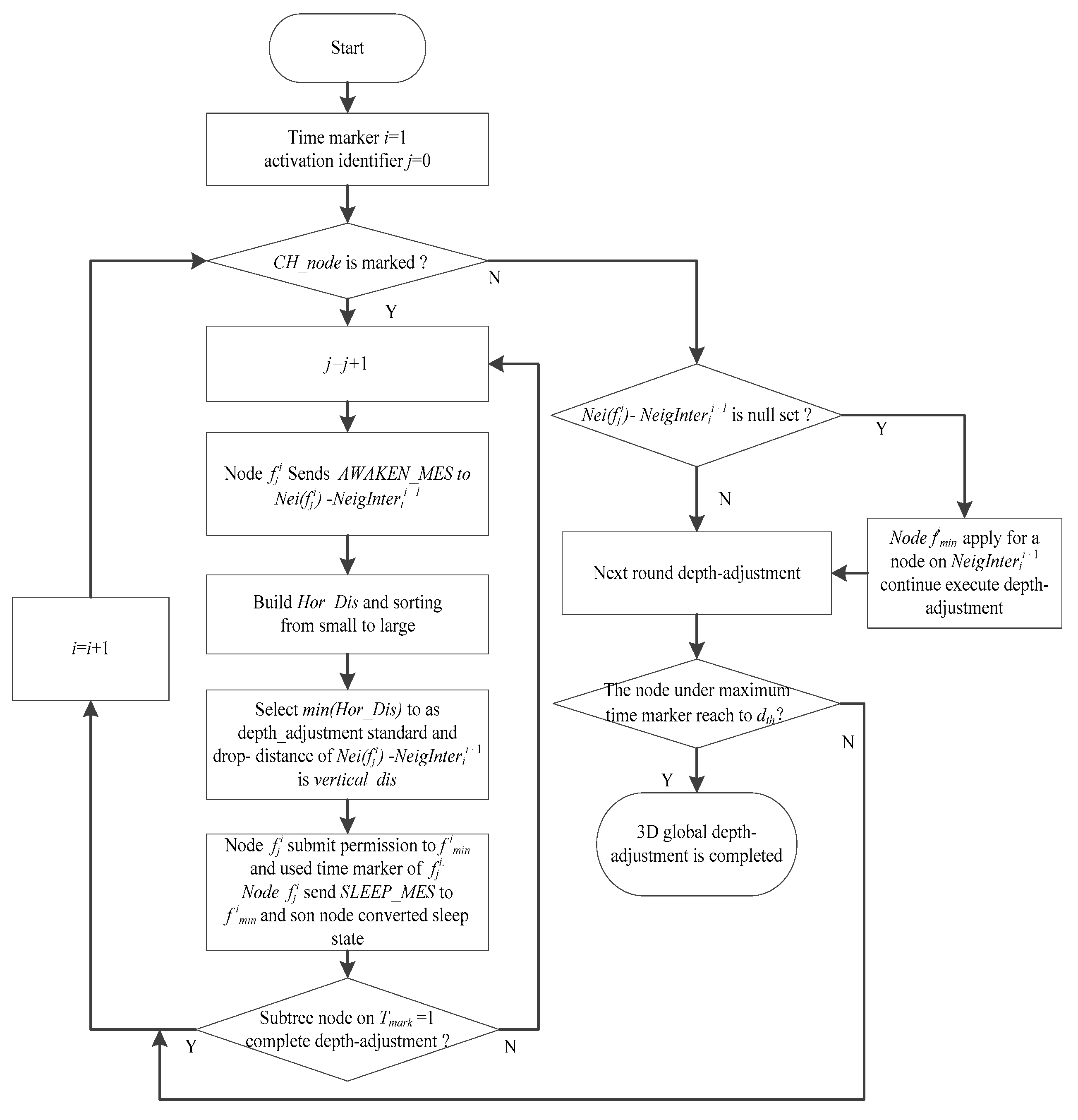
- The horizontal distance state table Hor_Dis(fji, Nei(fji) − NeigInterii+1) is updated, and node fimin is adopted according to Steps (2) and (3) to achieve the next layer of the depth adjustment of its child node continually. If the node in this time marker drops down to a depth threshold dth, then the depth adjustment on this time marker is completed. If the process finds no node to execute depth adjustment, that is, the set of neighbor nodes Nei(fji) − NeigInterii+1 is a null set, then node fimin applies to request other nodes in the set of neighbor intersections NeigInterii+1 to continue the process of depth adjustment until all child nodes of the entire time marker complete the whole depth-adjustment process, finishing the global 3D network coverage deployment. The flowchart of the depth-adjustment strategy is shown in Figure 8.
5. Complexity Analysis
5.1. Communication Complexity Analysis
5.2. Time Complexity Analysis of Network Deployment
6. Simulation Evaluation
6.1. Parameter Settings and Evaluation Metrics
6.2. Comparison and Analysis of Simulation Results
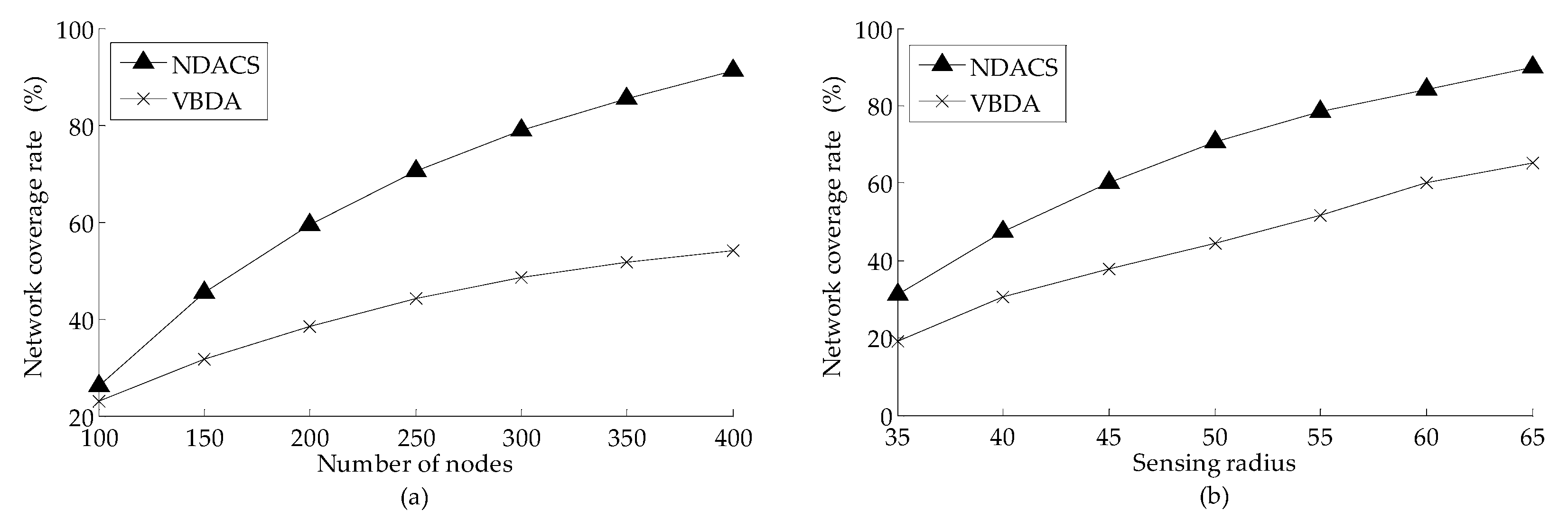
6.2.1. Network Coverage Rate
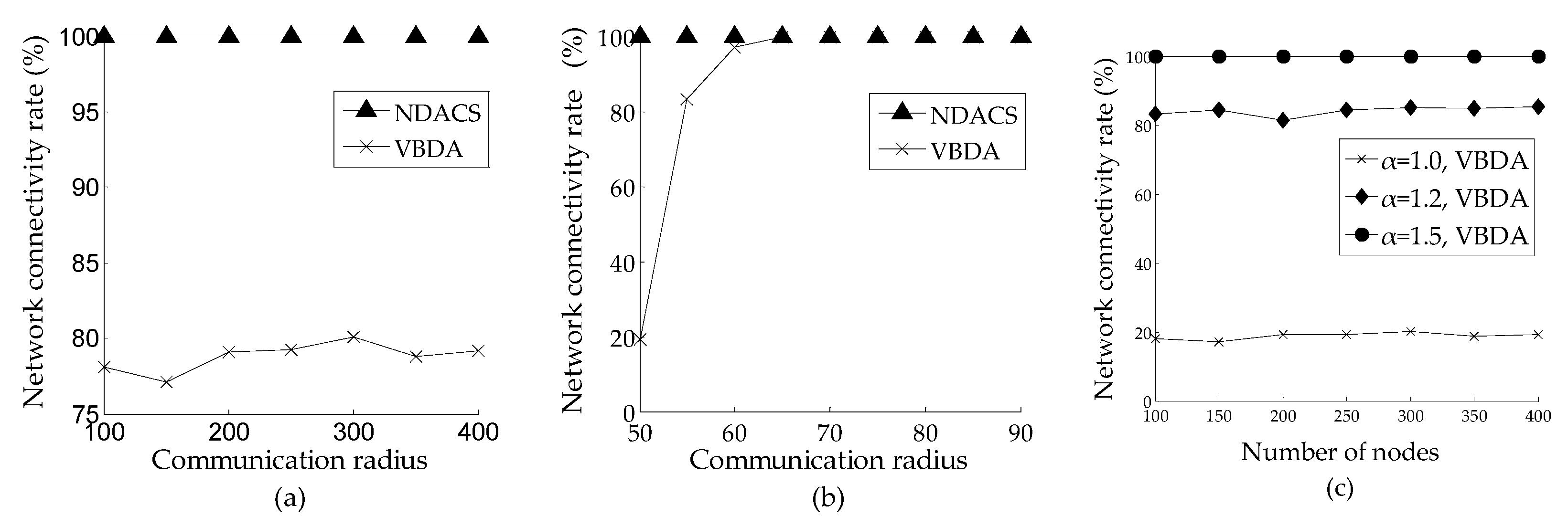
6.2.2. Network Connectivity Rate
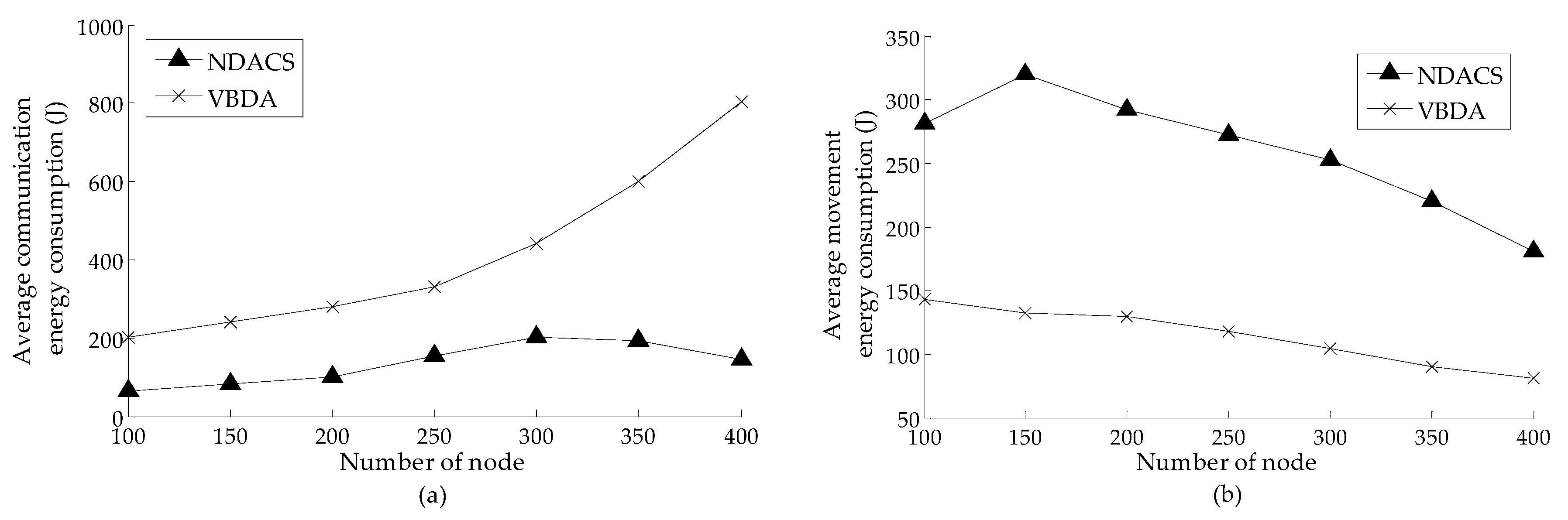
6.2.3. Energy Consumption of Communication and Movement
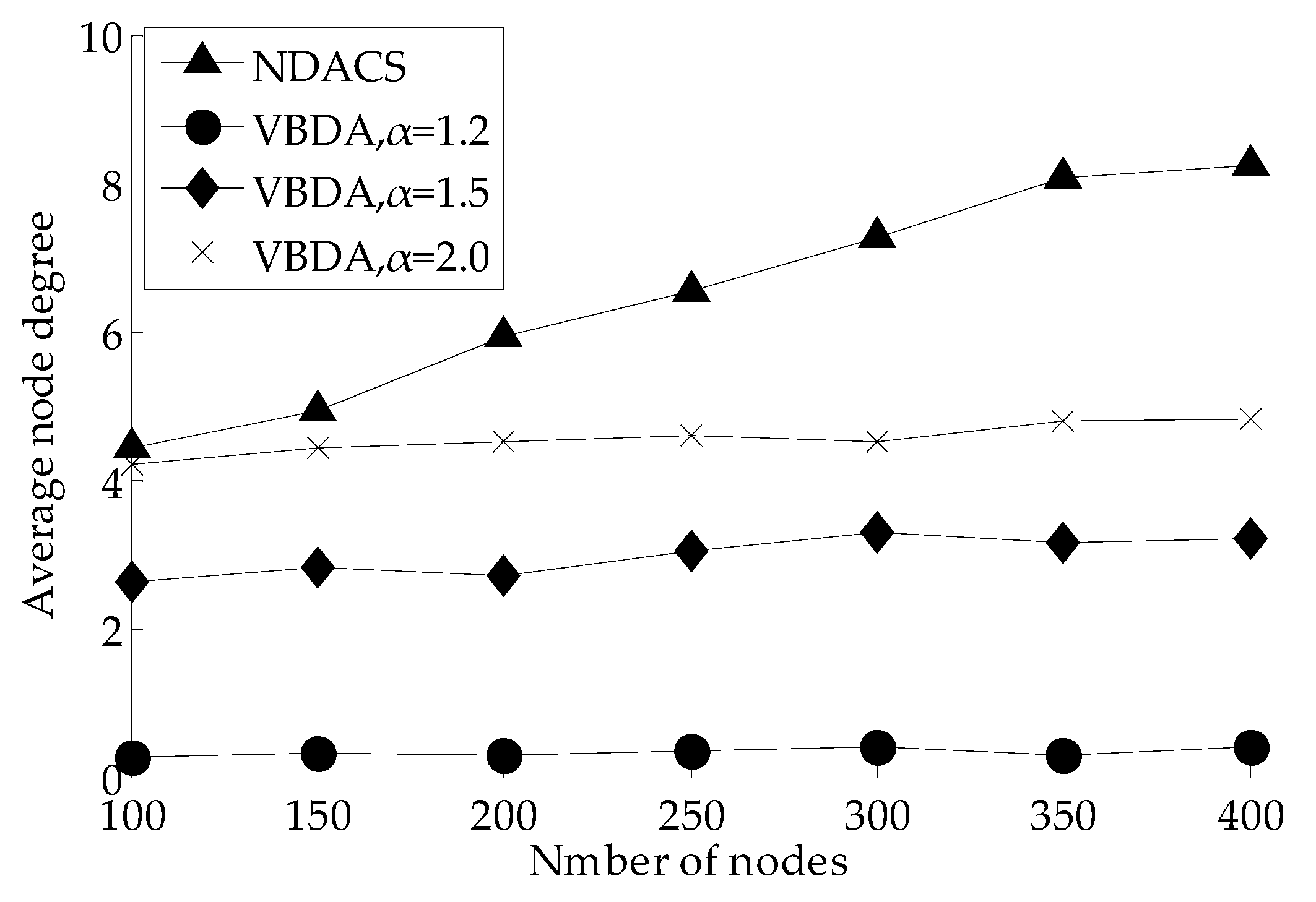
6.2.4. Network Reliability
7. Conclusions
Acknowledgments
Author Contributions
Conflicts of Interest
References
- Heidemann, J.; Stojanovic, M.; Zorzi, M. Underwater sensor networks: Applications, advances and challenges. Philos. Trans. R. Soc. A Math. Phys. Eng. Sci. 2012, 370, 158–175. [Google Scholar] [CrossRef] [PubMed]
- Gkikopouli, A.; Nikolakopoulos, G.; Manesis, S. A survey on underwater wireless sensor networks and applications. In Proceedings of the IEEE Conference on Control and Automation (MED), Barcelona, Spain, 3–6 July 2012; pp. 1147–1154.
- Heidemann, J.; Ye, W.; Wills, J. Research challenges and applications for underwater sensor networking. In Proceedings of the IEEE Conference on Wireless Communications and Networking (WCNC), Las Vegas, NV, USA, 4–5 April 2006.
- Bhambri, H.; Swaroop, A. Underwater sensor network: Architectures, challenges and applications. In Proceedings of the IEEE International Conference on Computing for Sustainable Global Development, New Delhi, India, 5–7 March 2014; pp. 915–920.
- Huang, X.; Zhang, X. A Node Deployment Algorithm Based on Van Der Waals Force in Wireless Sensor Networks. Int. J. Distrib. Sens. Netw. 2013, 2013. [Google Scholar] [CrossRef]
- Temel, S.; Unaldi, N.; Kaynak, O. On deployment of wireless sensors on 3-D terrains to maximize sensing coverage by utilizing cat swarm optimization with wavelet transform. IEEE Trans. Syst. Man Cybern. Syst. 2014, 44, 111–120. [Google Scholar] [CrossRef]
- Manvi, S.; Manjula, B. Issues in underwater acoustic sensor networks. Int. J. Comput. Electr. Eng. 2011, 3, 101–111. [Google Scholar]
- Guerriero, F.; Violi, A.; Natalizio, E. Modelling and solving optimal placement problems in wireless sensor networks. Appl. Math. Model. 2011, 35, 230–241. [Google Scholar] [CrossRef]
- Cai, S.B.; Zhang, G.Z.; Liu, S.L. Weighted Localization for Underwater Sensor Networks. Lect. Notes Electr. Eng. 2014, 295, 325–334. [Google Scholar]
- Huang, C.J.; Wang, Y.W.; Lin, C.F. A self-healing clustering algorithm for underwater sensor networks. Clust. Comput. 2011, 14, 91–99. [Google Scholar] [CrossRef]
- Cheng, W.; Teymorian, A.Y.; Ma, L. Underwater Localization in Sparse 3D Acoustic Sensor Networks. In Proceedings of the 27th Conference on Computer Communications, Phoenix, AZ, USA, 13–18 April 2008.
- Han, G.; Zhang, C.; Shu, L. A survey on deployment algorithms in underwater acoustic sensor networks. Int. J. Distrib. Sens. Netw. 2013, 2013. [Google Scholar] [CrossRef]
- Pompili, D.; Melodia, T.; Akyildiz, I.F. Deployment analysis in underwater acoustic wireless sensor networks. In Proceedings of the 1st ACM International Workshop on Underwater Networks, Los Angeles, CA, USA, 25 September 2006; pp. 48–55.
- Akkaya, K.; Newell, A. Self-deployment of sensors for maximized coverage in underwater acoustic sensor networks. Comput. Commun. 2009, 32, 1233–1244. [Google Scholar] [CrossRef]
- Senel, F.; Akkaya, K.; Erol-Kantarci, M.; Yilmaz, T. Self-deployment of mobile underwater acoustic sensor networks for maximized coverage and guaranteed connectivity. Ad Hoc Netw. 2014, 34, 170–183. [Google Scholar] [CrossRef]
- Alam, S.M.; Haas, Z.J. Coverage and connectivity in three-dimensional networks. In Proceedings of the 12th annual international conference on Mobile computing and networking, Los Angeles, CA, USA, 24–29 September 2006; pp. 346–357.
- Alam, S.M.N.; Haas, Z.J. Coverage and connectivity in three-dimensional networks with random node deployment. Ad Hoc Netw. 2015, 34, 157–169. [Google Scholar] [CrossRef]
- Liu, L. A deployment algorithm for underwater sensor networks in ocean environment. J. Circuits Syst. Comput. 2011, 20, 1051–1066. [Google Scholar] [CrossRef]
- Xia, N.; Wang, C.S.; Zheng, R.; Jiang, J.G. Fish Swarm Inspired Underwater Sensor Deployment. Acta Autom. Sin. 2012, 38, 295–302. [Google Scholar] [CrossRef]
- Du, H.; Xia, N.; Zheng, R. Particle Swarm Inspired Underwater Sensor Self-Deployment. Sensors 2014, 14, 15262–15281. [Google Scholar] [CrossRef] [PubMed]
- Li, X.Y.; Ci, L.L.; Yang, M.H.; Tian, C.P.; Li, X. Deploying three-dimensional mobile sensor networks based on virtual forces algorithm. Commun. Comput. Inf. Sci. 2013, 334, 204–216. [Google Scholar]
- Heo, N.; Varshney, P.K. Energy-efficient deployment of intelligent mobile sensor networks. IEEE Trans. Syst. Man Cybern. Part A Syst. Hum. 2005, 35, 78–92. [Google Scholar] [CrossRef]
- Wang, G.; Cao, G.; La, P.T. Movement-assisted sensor deployment. IEEE Trans. Mob. Comput. 2006, 5, 640–652. [Google Scholar] [CrossRef]
- Wu, J.; Wang, Y.; Liu, L. A Voronoi-Based Depth-Adjustment Scheme for Underwater Wireless Sensor Networks. Int. J. Smart Sens. Intell. Syst. 2013, 6, 244–258. [Google Scholar]
- Jiang, P.; Xu, Y.; Wu, F. Node Self-Deployment Algorithm Based on an Uneven Cluster with Radius Adjusting for Underwater Sensor Networks. Sensors 2016, 16. [Google Scholar] [CrossRef] [PubMed]
- Jiang, P.; Wang, X.; Jiang, L. Node deployment algorithm based on connected tree for underwater sensor networks. Sensors 2015, 15, 16763–16785. [Google Scholar] [CrossRef] [PubMed]
- Jiang, P.; Liu, J.; Wu, F.; Wang, J.; Xue, A. Node Deployment Algorithm for Underwater Sensor Networks Based on Connected Dominating Set. Sensors 2016, 16. [Google Scholar] [CrossRef] [PubMed]
- Jiang, P.; Liu, J.; Wu, F. Node non-uniform deployment based on clustering algorithm for underwater sensor networks. Sensors 2015, 15, 29997–30010. [Google Scholar] [CrossRef] [PubMed]
- Partan, J.; Kurose, J.; Levine, B.N. A survey of practical issues in underwater networks. ACM SIGMOBILE Mob. Comput. Commun. Rev. 2006, 11, 23–33. [Google Scholar] [CrossRef]
- Ahmed, S.; Javaid, N.; Khan, F.A. Co-UWSN: Cooperative Energy Efficient Protocol for Underwater WSNs. Int. J. Distrib. Sens. Netw. 2015, 75. [Google Scholar] [CrossRef] [PubMed]
- Wang, P.; Li, C.; Zheng, J. A Dependable Clustering Protocol for Survivable Underwater Sensor Networks, Communications. In Proceedings of the IEEE International Conference on Communications, Beijing, China, 19–23 May 2008; pp. 3263–3268.
- Saxena, S.; Mishra, S.; Singh, M. Clustering Based on Node Density in Heterogeneous Under-Water Sensor Network. Int. J. Inf. Technol. Comput. Sci. 2013, 5, 49–55. [Google Scholar] [CrossRef]
- Preparata, F.P.; Hong, S.J. Convex hulls of finite sets of points in two and three dimensions. Commun. ACM 1977, 20, 87–93. [Google Scholar] [CrossRef]
- Rachman, R.; Laksana, E.P.; Putra, D.S. Energy Consumption at the Node in Underwater Wireless Sensor Network (UWSNs). In Proceedings of the 6th UKSim/AMSS European Symposium on Computer Modeling and Simulation IEEE Computer Society, Valetta, Malta, 14–16 November 2012; pp. 418–423.


| H | Depth of Monitoring Space |
|---|---|
| v | Movement speed of node |
| K | Number of times of depth-adjustment |
| Rc | Communication radius of node |
| P | Speed of sound |
| Td | Propagation delay of acoustic signal |
| Tc | Transition time from active to sleep or inversely |
| Parameter | Value |
|---|---|
| Initial energy of node Einit | 16,000 J |
| Coverage threshold Cth | 0.9 |
| Energy consumption on unit moving distance mu | 2 J/m |
| Power threshold P0 | 0.05 W |
| Transmission delay Tp | 0.2 s |
| Energy spreading factor k | 2 |
| Carrier frequency f | 24 kHz |
| Sense radius of node Rs | 50 m |
| Symbol | Definition |
|---|---|
| N | Number of nodes |
| ID | Node unique identifier |
| Rs | Node sensing radius |
| Rc | Node communication radius |
| Rcinit | Initial communication radius |
| Adjustable level of communication radius | |
| Bu | Accumulation of communication radius |
| Si | ID is i of node |
| D | Transmitting distance of the information package |
| P0 | Power threshold of packets can be received |
| F | Carrier frequency |
| Tp | Transmission delay of data transmission |
| K | Energy spreading factor |
| Me | Movement energy consumption of node |
| md | Node movement distance |
| mu | Energy consumption on unit moving distance |
| Ss | Set of sleep nodes |
| Sa | Set of active nodes |
| sleep_in | Set of sleep nodes inside the convex hull |
| sleep_out | Set of sleep nodes outside the convex hull |
| Sc | Network coverage area on process of convex hull activation |
| SCH | Area of 2d convex hull |
| SHole | Area of coverage holes |
| Rh | Empty circle radius |
| NA | Total number of active nodes |
| Nei_A | Active neighbor nodes set |
| Nei(fji) | Neighbor nodes set of node fji |
| NeigInterii+1 | Insertion of neighbor sleep nodes |
| {fji} | Parent node set of subtree |
| Tmark | Time marker of active node |
| dth | Depth-adjustment threshold of network |
| Cth | Coverage threshold on 2d network surface |
| IDA | Activation identifier of node |
| Cc | Network coverage rate |
| Cn | Network connectivity rate |
| Α | Ratio of node communication radius to sensing radius |
© 2016 by the authors; licensee MDPI, Basel, Switzerland. This article is an open access article distributed under the terms and conditions of the Creative Commons Attribution (CC-BY) license (http://creativecommons.org/licenses/by/4.0/).
Share and Cite
Jiang, P.; Liu, S.; Liu, J.; Wu, F.; Zhang, L. A Depth-Adjustment Deployment Algorithm Based on Two-Dimensional Convex Hull and Spanning Tree for Underwater Wireless Sensor Networks. Sensors 2016, 16, 1087. https://doi.org/10.3390/s16071087
Jiang P, Liu S, Liu J, Wu F, Zhang L. A Depth-Adjustment Deployment Algorithm Based on Two-Dimensional Convex Hull and Spanning Tree for Underwater Wireless Sensor Networks. Sensors. 2016; 16(7):1087. https://doi.org/10.3390/s16071087
Chicago/Turabian StyleJiang, Peng, Shuai Liu, Jun Liu, Feng Wu, and Le Zhang. 2016. "A Depth-Adjustment Deployment Algorithm Based on Two-Dimensional Convex Hull and Spanning Tree for Underwater Wireless Sensor Networks" Sensors 16, no. 7: 1087. https://doi.org/10.3390/s16071087
APA StyleJiang, P., Liu, S., Liu, J., Wu, F., & Zhang, L. (2016). A Depth-Adjustment Deployment Algorithm Based on Two-Dimensional Convex Hull and Spanning Tree for Underwater Wireless Sensor Networks. Sensors, 16(7), 1087. https://doi.org/10.3390/s16071087