Abstract
The aim of this paper is to improve the position accuracy of a six degree of freedom medical robot. The improvement in accuracy is achieved without the use of any external measurement device. Instead, this work presents a novel calibration approach based on using an embedded force-torque sensor to identify the robot’s kinematic parameters and thereby enhance the positioning accuracy. A simulation study demonstrated that our calibration approach is effective, whether or not any measurement noise is present: the position error is improved, inside the robot target workspace, from 12 mm to 0.320 mm, for the maximum values, and from 9 mm to 0.2771 mm, for the mean errors.
1. Introduction
Medical robots show a promising future in various health issues in the most recent decades. With recent developments in sensors and control theory, medical robots provide many inspiring solutions in the fields of: diagnosis, surgery, orthopedics, rehabilitation, prosthetics and exoskeletons, etc. [1,2]. The force-torque (wrench) sensor is an essential component of these medical robot applications. MedRUE [3], OTELO [4] and Hippocrate [5] robot systems were developed for the ultrasound scanning of vascular diseases. In all three robot systems, force-torque sensors are employed to maintain proper contact with the patient’s body during the examination. The Black Falcon system, which is a fundamental study for many other surgical robot systems, allows the surgeon to feel the interaction with tissue and thereafter improve the surgical performance. The Da Vinci system is a popular surgery robot widely used in hospitals [6]. The adoption of force-torque sensors in Da Vinci system has been studied in depth [7]. The Robodoc assistant system is a medical orthopedic robot for use during total knee replacement, and it achieves results that are comparable to technician performance [8]. The force-torque sensors are used in Robodoc for both control and safety reasons.
Medical robots have also contributed to the field of rehabilitation. The InMotion ARM, which is based on the MIT-Manus project, is an interactive robotic system for upper-extremity rehabilitation therapy [9,10], and the robotic stepper is a device, developed by the National Aeronautics and Space Administration (NASA), to help patients with lower-extremity rehabilitation [11]. Force-torque sensors are employed in these rehabilitation robots to measure the strength and the capability of the patient. Medical robots have also been developed as substitutes for malfunctioning parts of the human body. The I-limb ultrasound system and the ReWalk system are exoskeleton robots for hand prosthetics and leg prosthetics, respectively [12,13]. Force-torque sensors are used in the prosthetic and exoskeleton robots to control the joints and to evaluate the power of the limb movements.
Medical robots often need to be accurate, not just repeatable, which means that they must be calibrated. Most robot calibration approaches are based on minimizing the pose residual, which involves external measurement devices such as a coordinate measurement machine (CMM) [14,15], laser tracker [16,17,18], measurement articulated arm [14], ball-bar [19,20], or a high-accuracy touch probe [21,22]. However, these measurement devices tend to be expensive, and they are not readily available. Furthermore, even though other studies have developed low-cost calibration methods, such as in [19,20], they still require the use of external measurement devices.
Other robotic applications are dedicated to measuring and/or reproducing human movements, such as [23], which presents a methodology to accurately record human finger postures during grasping. In this work, human finger postures are measured during grasping. As with the aforementioned works, measurements are taken with external measurement devices: an optical tracking of markers that are attached to the skin of the hand, and tracked using stereo-cameras. The considered kinematic parameters in this work are geometric static parameters, and parameters controlling the location of the bones and the joint markers. These parameters are identified by using a constrained least-squares minimization. The minimization problem is solved by employing a primal-dual interior point. It minimizes the residuals of the coordinates of measured markers and the corresponding estimated coordinates, which are a function of the static parameters and joint angle values.
Force-torque sensors are already used in many medical robot systems, so it makes sense to use these sensors, rather than external coordinate measurement equipment, for calibrating the robots (i.e., improving the robot positioning accuracy). Yet, to the best of our knowledge, no such calibration methods have been proposed in the literature. In previous work, other measurement approaches were used, such as Cartesian coordinates [14,15,16,17,18], or distance measurements [19,20]. The novelty of our work is the use of a force-torque sensor to improve the positioning accuracy of a medical robot (MedRUE). The robot parameters are identified by minimizing the force and torque residuals, instead of minimizing the residuals of the end-effector position and/or orientation, as done in conventional approaches [14,15,16,17,18,19,20]. The sensor we used is the embedded force-torque sensor, located between the flange and the tool. Thus, our calibration approach can be considered as a self-calibration method.
The proposed approach could be used for any other medical or industrial robot. Industrial robots are not always equipped with force-torque sensors. However, such sensors are readily available in the market and can be easily installed. Indeed, industrial serial robots are increasingly using these sensors for programming purposes: the force-torque sensors are installed in order to move manually the robot end-effector, during the online programming (also called lead-through programming).
In the identification process proposed in this paper, the data are collected by the robot’s force-torque sensor. The process of identifying the parameters is based on minimizing the residual of the force and torque at the robot’s end-effector. The accurate identification of the robot’s parameters leads to improved position accuracy. Our approach is validated through a simulation, in which the position accuracy is evaluated before and after calibration.
This paper is organized as follows. The next section describes the force and torque forward kinematic equations, followed by a description of the calibration approach. We then present our simulation study, followed by a results analysis. Finally, we discuss our conclusions and suggestions for further work in the last section of the paper.
2. Robot Description and Forward Kinematics
2.1. Robot Description and the Main Reference Frames
The MedRUE robot (Figure 1a) is a medical robot dedicated for vascular ultrasound examination. MedRUE is a six degrees of freedom (6-DOF) hybrid serial-parallel robot. It is composed of two five-bar mechanisms (Figure 1b), which are symmetrically assembled. These mechanisms are considered to be perfectly parallel to each other and perpendicular to the robot base. The robot base is fixed to a linear guide actuated through a servomotor SM1; the corresponding joint variable is denoted by q1. Five other servomotors are also used in order to actuate the robot revolute joints: SM2 and SM3, for the left five bar mechanism, and SM4 and SM5 for the right side (Figure 1a). The sixth servomotor—attached to the link having as its length—is used to rotate the probe about the x axis of the last reference frame (F6), which is defined as follows: the origin of F6 is located midway between G1 and G2; its x axis (x6) is defined to pass through G1 and G2, and z6 is pointing toward the probe center.
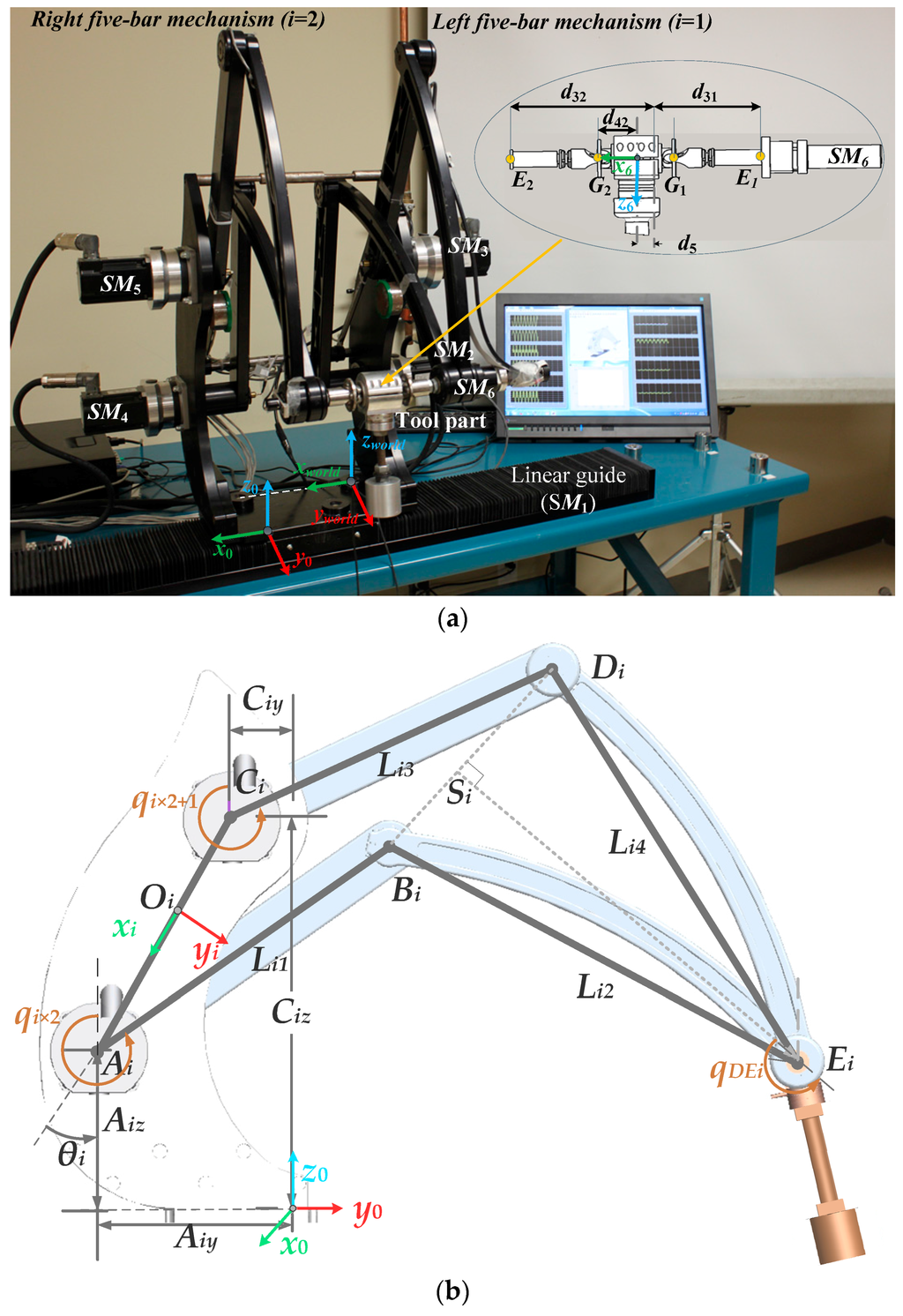
Figure 1.
(a) The MedRUE robot prototype with the tool part and (b) a five-bar mechanism of the MedRUE where (i = 1, 2).
Each five-bar mechanism i (i = 1, 2) has five links: the distance di between the anchor points of the two proximal links, and the four mobile links having Lij (j = 1, 2, 3, 4) as lengths. The five links connect five revolute joints (Ai, Bi, Ci, Di, Ei), among which only two (Ai and Ci) are actuated through servomotors SMi×2 and SMi×2+1: the corresponding two angles are denoted qi×2 and qi×2+1, respectively. A total of five angles of active joints are considered (q2, …, q6).
Finally, joints E1 and E2 are linked through the probe support (Figure 1a), which has a universal joint at each extremity Gi. The x coordinate of Gi with respect to the base frame is denoted by .
In our calibration process, nine reference frames are considered:
- F0: The reference frame of the robot base, located on the robot base at O0. As shown in Figure 1a, the x axis (x0) is aligned with the axis of the linear guide, and z0 is normal to the plane defined by the platform of the robot base. The translation and the orientation (α0, β0, γ0), described in XYZ fixed Euler angles, of F0 with respect to Fworld, are expected to be identified by the calibration process.
- Fworld: The world reference frame (Figure 1a), associated with the robot work-cell. It has approximately the same orientation as F0.
- F1 to F6: The reference frames associated with the joints (F1, F2, …, F6). These frames are not shown.
- Ftool: The tool reference frame associated with the robot probe (Figure 2). The origin of Ftool is described to be the center of the end-effector (i.e., the probe), and its orientation is considered to be the same as that of F6. Knowing that the end-effector orientation is not used in our calibration process, therefore, only the translation of Ftool with respect to F6 is considered.
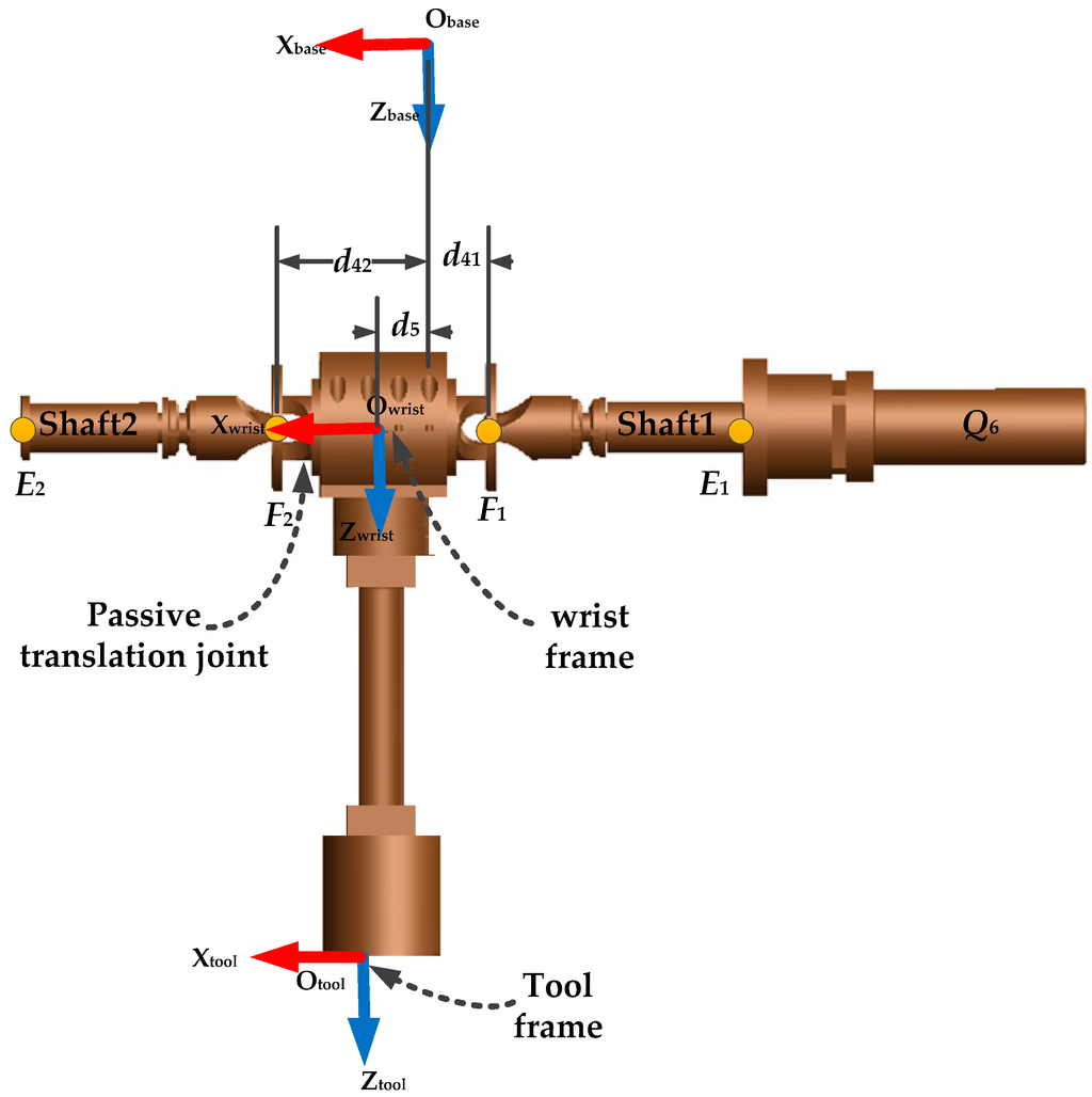 Figure 2. Tool part of MedRUE.
2.2. Position Equations
Given the vector ψ = [q1, q2, …, q6]T of the active joint variables, the end-effector’s pose with respect to the world frame is represented by homogeneous matrices as follows:
where denotes the homogeneous matrix representing a frame a with respect to a frame b, and can be represented in the matrix form of .
The rotation matrix is often represented by R(α,β,γ) = Rx(γ)Ry(β)Rz(α), and the translation matrix by T(x,y,z) = Tx(x)Ty(y)Tz(z), where Ru(ϕ) and Tu(d) are the rotation/translation operator along the u axis with value ϕ/d. Since robot joints are only included in , then , and in Equation (1) are constant matrices, which can be defined directly by parameter sets [x0, y0, z0, α0, β0, γ0], [xS, yS, zS, αS, βS, γS] and [xT, yT, zT, αT, βT, γT]. The following paragraphs present the calculation of .
The coordinates of and are expressed with respect to the local frame Fi on ith five-bar mechanism as follows:
where Li1 and Li3 are the lengths of the four swinging links as shown in Figure 1, and is the offset of ith active joint. The vector is calculated as follows:
and
The coordinates of with respect to a frame Fi are obtained as follows:
where
and is the unit vector along .
The coordinates of w.r.t. Fbase are obtained by a transformation matrix as follows:
where
and θi, which is the angle between and the normal of the x0y0 plane, is calculated as follows:
The orientation of Fwrist w.r.t. Fbase is obtained from the corresponding rotation matrix , where α, β and γ are the fixed XYZ Euler angles. The rotation angle along x0 is directly obtained as . According to the design of the tool part shown in Figure 2,
Then α and β are obtained as:
where, .
The translation of Fwrist w.r.t. Fbase is calculated as follows:
Finally, the pose of Fwrist w.r.t. Fbase is expressed as follows:
2.3. Force and Torque Equations
The gravity frame Fgravity is assigned at the tool part’s center of gravity, as shown in Figure 3. When the robot is not in contact with its environment, the gravity force fG in frame Fgravity is the cause of the force and torque on the force sensor. The forward kinematic solution to obtain the force and torque in force sensors is:
where is a 6 × 1 wrench vector composed of force and torque, and is a 6 × 6 transformation matrix between screws. The orientation of Fgravity is in alignment with Fworld, rather than fixed relative to the tool part. The wrench of the gravity force of the tool part w.r.t. the Fgravity is
where with mTool is the mass of the tool part and g is the gravitational constant. Since gravity is a pure force, .
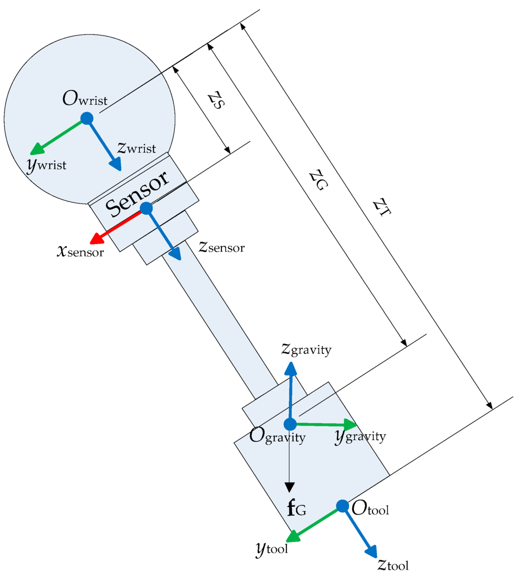
Figure 3.
Gravity effect of the tool part on the force sensor.
The transformation matrix can be expressed as
Since Fgravity keeps the same orientation with Fworld, then . is the translation offset of the origin of Fgravity w.r.t. Fwrist. is the vector product operation, and it is equal to
Similar to Equation (19), is characterized by parameters describing Fsensor w.r.t. Fwrist:
The sensor reference frame Fsensor is defined in the information given by the sensor manufacturer. During assembly, its orientation w.r.t. Fwrist is expressed by Euler-XYZ angles:
Similar to Equation (20), is the vector product operation of .
3. Parameters Used During Calibration
In our robot calibration process, the following parameters were considered:
- The lengths of the ten links of the two five-bar mechanisms: L11, L12, L13, L14, L21, L22, L23 and L24.
- The y and z coordinates of the anchor points of the two proximal links of the five-bar mechanisms: A1y, A1z, C1y, C1z, A2y, A2z, C2y, C2z.
- The offsets of the six active joints: δq1, δq2, δq3, δq4, δq5, δq6.
- The offset parameters for the tool part: d31, d32, d41, d42, d5.
- The parameters defining the base with respect to the world frame: x0, y0, z0, α0, β0, γ0.
- The position of the tool frame with respect to the wrist frame: xT, yT, zT, αT, βT, γT.
- The parameters to describe the sensor frame w.r.t. the wrist frame: xS, yS, zS, αS, βS, γS.
- The parameters to describe the offset of gravity frame w.r.t. the wrist frame: xG, yG, zG.
- The mass of the tool part: mTool.
Of the 46 parameters that we considerd, a total of 17 parameters are non-identifiable, which means that we need to reduce the number of identifiable parameters to 29.
4. Calibration Process
Our calibration process is explained in detail in Section 4.1, Section 4.2 and Section 4.3. Its main steps are presented in what follows:
- Develop the calibration model: the forward kinematics, presented in Section 2.2.
- Create a pool Ω of 40,000 configurations uniformly distributed inside the whole robot workspace. Create a set Ωt of 336 configurations uniformly distributed inside the target workspace (see Section 4.3). We note that the configurations of the set Ωt are different from these of Ω.
- Select 100 configurations to be used in the identification process. These configurations are chosen through an observability analysis, as explained in Section 4.1.
- Take the force and torque measurements, for all robot configurations (Ωt and Ω). Measurements are done by using the robot force-torque sensor. We note that in this paper all measurements are generated by simulation, as explained in Section 4.3 and Section 5.
- Identify the robot parameter values by using the calibration configurations selected in step 3; the identification approach is presented in details in Section 4.2.
- Evaluate the accuracy after calibration, as explained in Section 5.
4.1. Selection of Calibration Configurations
After creating the calibration model, and generating a pool Ω of 40,000 configurations uniformly distributed inside the whole robot workspace, a set of 100 calibration configurations is selected among Ω. This is done by using an approach commonly called observability analysis. This analysis is used to obtain the optimal set of the calibration configurations, and is based on the singular value decomposition (SVD) of the identification Jacobian matrix J. The matrix J is composed of the derivatives of the end-effector force and torque vector (Equation (17)), with respect to all of the robot independent parameters. The Jacobian matrix is also used in the linearization of the force and torque equations (Equation (17)), around the calibration configurations (i.e., Taylor approximation). This linearization allows identifying the parameter values, as explained in Section 4.2. The nominal values of the robot’s independent parameters are represented by the vector pnom. The matrix J is calculated as follows, for i = 1…n.
where Ji is the 6 × m Jacobian matrix at the ith calibration configuration, n is the number of calibration configurations, and m is the number of considered parameters (not all of which are necessarily identifiable). In our case, n = 100 and m = 49.
Ji is given by:
The matrix J is also used to find the non-identifiable parameters. The rank rJ of the Jacobian J represents the number of identifiable parameters. If rJ < m, then m − rJ parameters are non-identifiable; the corresponding columns should be removed from J. This procedure is carried out using an algorithm that is based on the approach proposed in [21]. The stop criteria is when m becomes equal to rJ. The algorithm proceeds as follows:
- Remove all zero columns from J. The corresponding parameters have no impact on the calibration model.
- Calculate the condition number, cJ, of J. The condition number is used to evaluate how good is the matrix J for the parameter identification. With a bad condition number (high value), the solutions are unstable with respect to small changes in measurement errors. Therefore, to have a robust identification system, the condition number should be as small as possible.
- Remove, one at a time, the column related to each parameter from J, and calculate both the new rank and condition number ( and ) for the new Jacobian matrix J*. The column that, if eliminated, results in the maximum reduction of the condition number and gives the same rank ( = rJ), is definitively removed (i.e., the corresponding parameter will be not subject to the identification process).
- Replace J with J*, and repeat the process from step (2).
As a result, of the 49 parameters considered in our calibration model, 22 are non-identifiable and are indicated by the symbol ‘*’ in Table 1.

Table 1.
Results of the simulated parameter identification.
The fact that some parameters are non-identifiable is mainly due to redundancy, or the fact that they have no impact on the force and torque equations that represent the calibration model.
The parameter identification is achieved by minimizing the residual of the end-effector force and torque, which are measured by the robot’s force sensor (Figure 3); no external measurement device is required. Further, only the gravity effect of the end-effector is used to apply forces to the robot’s end-effector. Therefore, to change the applied force on the end-effector, it is necessary to change its orientation.
In our identification process, 100 calibration configurations are selected from among the 40,000 configurations. The remaining 39,900 configurations are used for validation purpose. The 40,000 configurations are uniformly distributed on three layers, within the entire robot workspace. Note that several orientations are generated for each position. The calibration configurations are selected using an observability analysis, which allows us to identify the most appropriate configurations and thus identify the most effective parameters. This analysis is based on using the first observability index, denoted by O1 and calculated by using the singular value of the Jacobian identification matrix (i.e., the sensitivity matrix). The procedure of selecting the calibration configurations is based on the DETMAX algorithm, which was initially proposed in [24].
According to [25,26], the index O1 seems to be the most appropriate index for the kinematic calibration. This was also confirmed by our simulation, through a comparison of the five observability indices that were presented in the literature and thoroughly detailed in [26]. The convergence of O1 is represented in Figure 4, and is calculated as follows:
where n is the number of calibration configurations, σ1 … σm are the singular values of the Jacobian identification matrix for the m = 29 identifiable parameters.
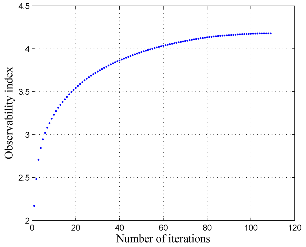
Figure 4.
Evolution of the observability index O1 with respect to the selection algorithm iterations.
4.2. Parameter Identification Process
The parameter identification process is based on using the Jacobian matrix J, which relates the force and torque errors to the 29 unknown parameter values. The matrix J is built by the linearization of the forward kinematics model (Equation (17)) around each calibration configuration. The parameter values are identified by means of an iterative algorithm, in which the parameters’ vector is initialized by pnom, and is updated at each iteration (i.e., replaced by the vector pidentified of the identified values). The matrix J is also iteratively updated, since its calculation is based on p.
The identification algorithm is presented in Figure 5 and has the following steps:
- (a)
- Matrix J is calculated, as explained in Section 4.1. This calculation involves p and the values of the vector ψi = [q1, q2,…, q6] T (i = 1,…, n) of active joints of the 100 calibration configurations.
- (b)
- A system of linear equations is formed by the measured force and torque errors, the unknown robot’s parameter errors, and the Jacobian matrix J. In order to maintain acceptable variance of each parameter (i.e., proper convergence in the linear system), parameter scaling is implemented, by using the column scaling approach proposed in [24]. The scaled matrix obtained is denoted by Jscal, and it is used to identify the robot’s scaled parameter errors (Δscal), as follows:where, [Fxmeas,i, Fymeas,i, Fzmeas,i, Txmeas,i, Tymeas,i, Tzmeas,i]T is the vector of the measured force and torque i, and [Fxest,i, Fyest,i, Fzest,i, Txest,i, Tyest,i, Tzest,i]T is the corresponding estimated vector. The estimated vector is calculated by substituting in the forward kinematic equation (Equation (17)): The vector p of the parameters’ values and the vector ψi of the active joint variables. The vector p is initialized by its nominal values pnom, and updated after each iteration of this identification algorithm.
- (c)
- The parameter errors, which represent the difference between the real values and the nominal values of the parameters, are denoted by Δ, and calculated as follows:where Dj, (j = 1, 2, …, m) are the scaling coefficients, defined as follows: . Also, n is the number of calibration configurations, and Jij is the element of the Jacobian matrix located at the ith row and the jth column.
- (d)
- Finally, the vector of the identified parameter values is
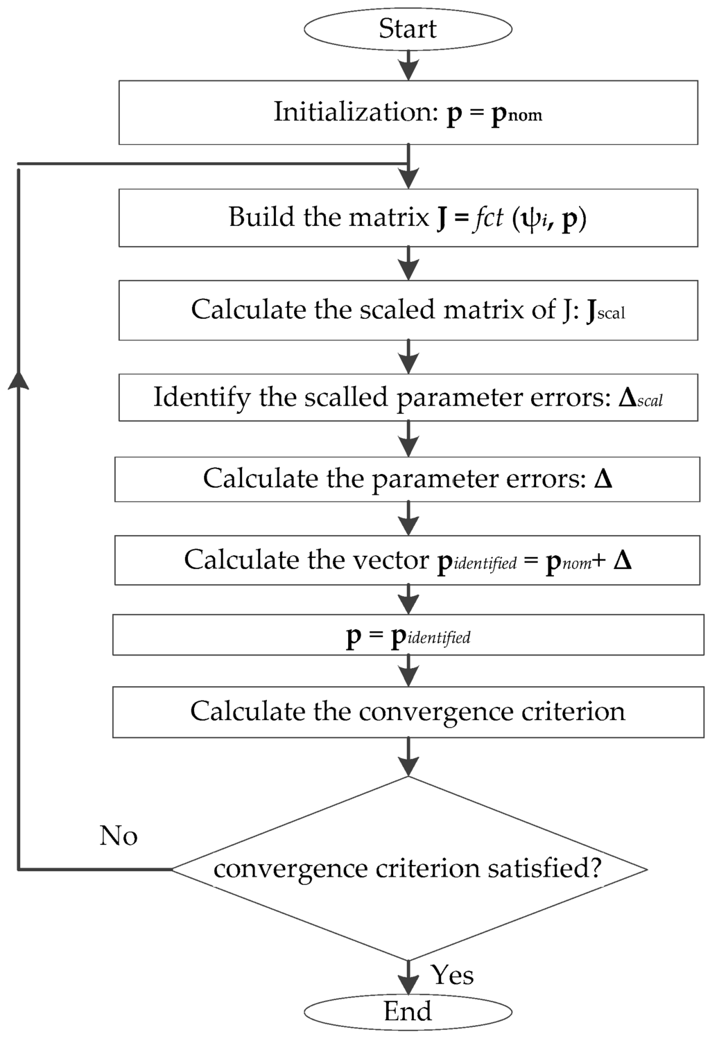
Figure 5.
Flow chart of the parameter identification algorithm.
To converge towards a solution for the unknown parameter values, an iterative Newton-based procedure was used. After pidentified has been calculated, the p vector is replaced by the last pidentified vector obtained, and the estimation process is restarted from step (a).
Steps (a) to (d) are repeated until reaching a convergence criterion, which is the root mean square error (RMSE) between two successive iterations. The RMSE is evaluated between the vector of the latest identified parameters and the previous one. The convergence criterion was set to 10−16, and the system converged towards a solution after five iterations.
4.3. Validation after Calibration
After calibration, the accuracy is validated using 336 configurations that are uniformly distributed inside the Cartesian target workspace. The target workspace is intended to correspond to the area where the patient’s leg will be located (Figure 6b). Also, the accuracy after calibration is evaluated by using the 39,900 configurations (denoted by Ωw), which are the remaining configurations among the initial set Ω composed of 40,000 configurations (Figure 6a) uniformly distributed within the whole robot workspace: 100 calibration configurations are selected from Ω, through the observability analysis, to be used in the parameter identification process, and 39,900 configurations are used in the validation after calibration.
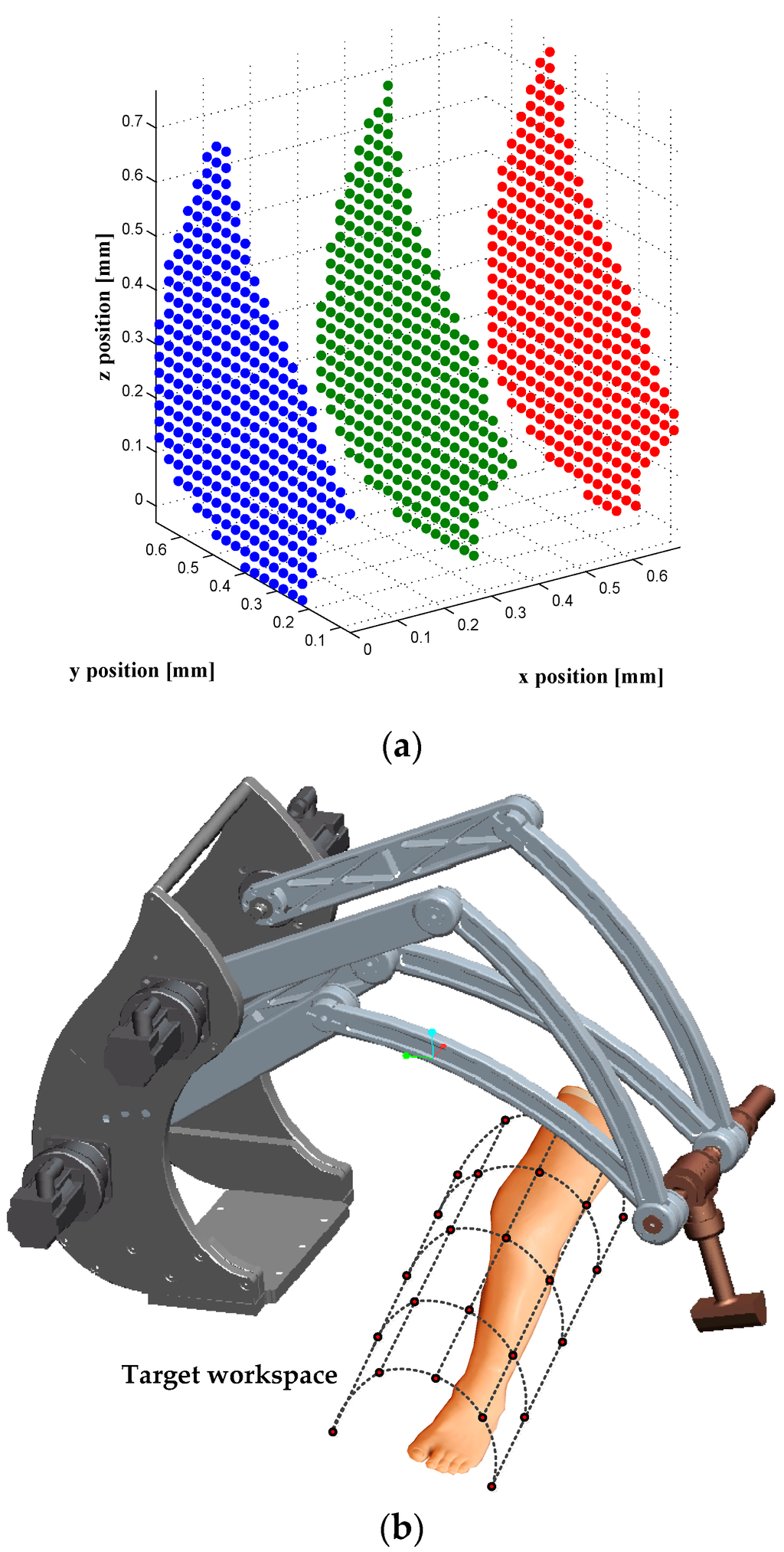
Figure 6.
The positioning of the robot end-effector within (a) the whole robot workspace; 40,000 configurations inside the whole robot workspace; and (b) the target workspace; 336 configurations inside the area where the patient’s leg will be located.
After achieving the parameter identification process, the identified parameters are used in the robot kinematics, instead of the nominal parameter values. The next step consists to evaluate the robot accuracy for all validation configurations (Ωw and Ωt), by using the following algorithm:
Loop 1
For each validation set, Ωw and Ωt:
Loop 2
For each validation configuration:
- (a)
- Calculate the desired position, by using the identified parameter values and the active joint angles ψ = [q1, q2,…, q6]T of the validation configuration. The end-effector position is the translation vector of the homogeneous matrix presented in Equation (1).
- (b)
- Calculate the actual position, by using the actual parameter values (generated by simulation) and the active joint angles of the calibration validation. In case of experimental tests, the actual position is obtained by measurement.
- (c)
- Calculate x, y, and z position errors (Ex, Ey, and Ez), by evaluating the difference between the desired and the actual position, obtained in steps (a) and (b), respectively.
- (d)
- Calculate the composed error () by using results obtained in step (c).
End Loop 2
Calculate the mean, the maximum and the standard deviation of all composed errors obtained in Loop 1.
End Loop 1
The force and torque validation is achieved by using the same algorithm as for position. The only difference is using Equation (17) instead of Equation (1), in step (a).
5. Simulation Study
The efficiency of our calibration process is evaluated through a simulation. This process also evaluates the sensitivity of our identification process to the measurement noise, and verifies the effectiveness of the observability analysis for choosing the calibration configurations. Finally, the calibration results (i.e., position accuracy) that were obtained from each of the five observability indices are compared, and the index that gives the best accuracy is used in the actual calibration.
For simulation purposes, the actual parameters’ values are simulated by introducing randomly-generated errors of ±2 mm for the distances, and ±1° for the angles. The differences between the nominal and the actual parameter errors simulate the behavior of a robot with poor accuracy. By using the calibration process, the identified parameters will be as close as possible to their actual values, despite the presence of the measurement errors. The measurement errors that were used in our simulation are ± 1 N and ± 0.2 N·m, for the force and torque, respectively. These errors are an exaggeration of the accuracy of the robot’s force-torque sensor (a Mini 40 from ATI), the details of which are provided by its manufacturer, through a calibration certificate. From this information, force accuracy according to x, y, and z axes was ± 0.25 N, ± 0.2 N, and ± 0.45 N, respectively. The torque accuracy was ± 0.0125 N.m, ± 0.0125 N.m, and ± 0.02 N.m, for x, y, and z axes.
The measurement errors are generated according to a normal distribution, for each axis (i.e., errors for Fx are generated within ± 1 N, and similarly for Fy and Fz). The data acquisition is simulated by generating 100 measurements (i.e., force and torque errors) for each calibration configuration of the robot. As it is known that the number of identifiable parameters is 29, the number of calibration configurations that are used in the identification process is 100, in order to over-constrain the calibration model.
The measured wrench vector (composed of force and torque) is simulated for each calibration configuration, by substituting the corresponding active joint angles and the actual parameter values (Table 1) in Equation (17). A vector of measurement noise is then added to the obtained wrench vector.
Once all force-torque vectors are generated, the robot parameters are identified as explained in Section 4.2. The identified parameter values are presented in Table 1.
Once the parameters have been identified, the calibration process is validated. This validation is carried out, as explained in Section 4.3, on two levels: the robot’s position accuracy is assessed in both the whole robot workspace (39,900 configurations) and by using the 336 positions that are uniformly distributed within the target workspace. The force, torque and position errors are summarized in Table 2 and Table 3, and it shows that the position accuracy was improved from 8.9135 mm before calibration to 286 µm, after calibration, inside the target workspace. The wrench errors (Table 4) were highly improved (better than the position accuracy improvement) because in our identification process, only the residuals of force and torque were minimized in the objective function Equation (26). The distribution of the robot’s position errors (before and after calibration) is presented in Figure 7 and Figure 8, which represent the number of occurrences (frequency) of robot xyz composed position errors that lie within the ranges of error, presented on the horizontal axis.
Table 2.
Composite force and torque errors before and after calibration.
Table 3.
Composite position errors before and after calibration.
Table 4.
Composite force, torque and position errors after calibration using the five observability indices.
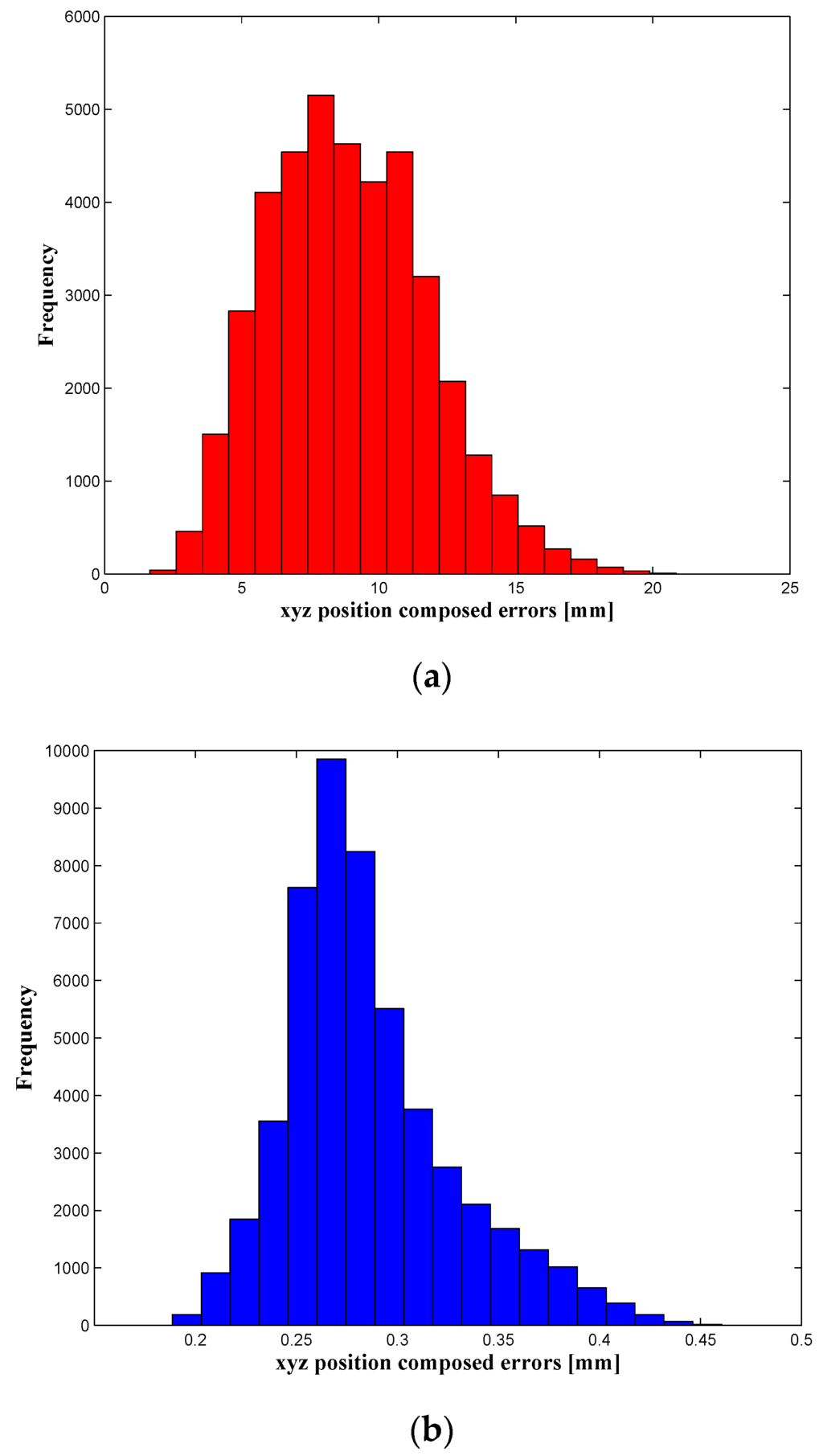
Figure 7.
Position errors in the whole workspace (a) before and (b) after calibration.
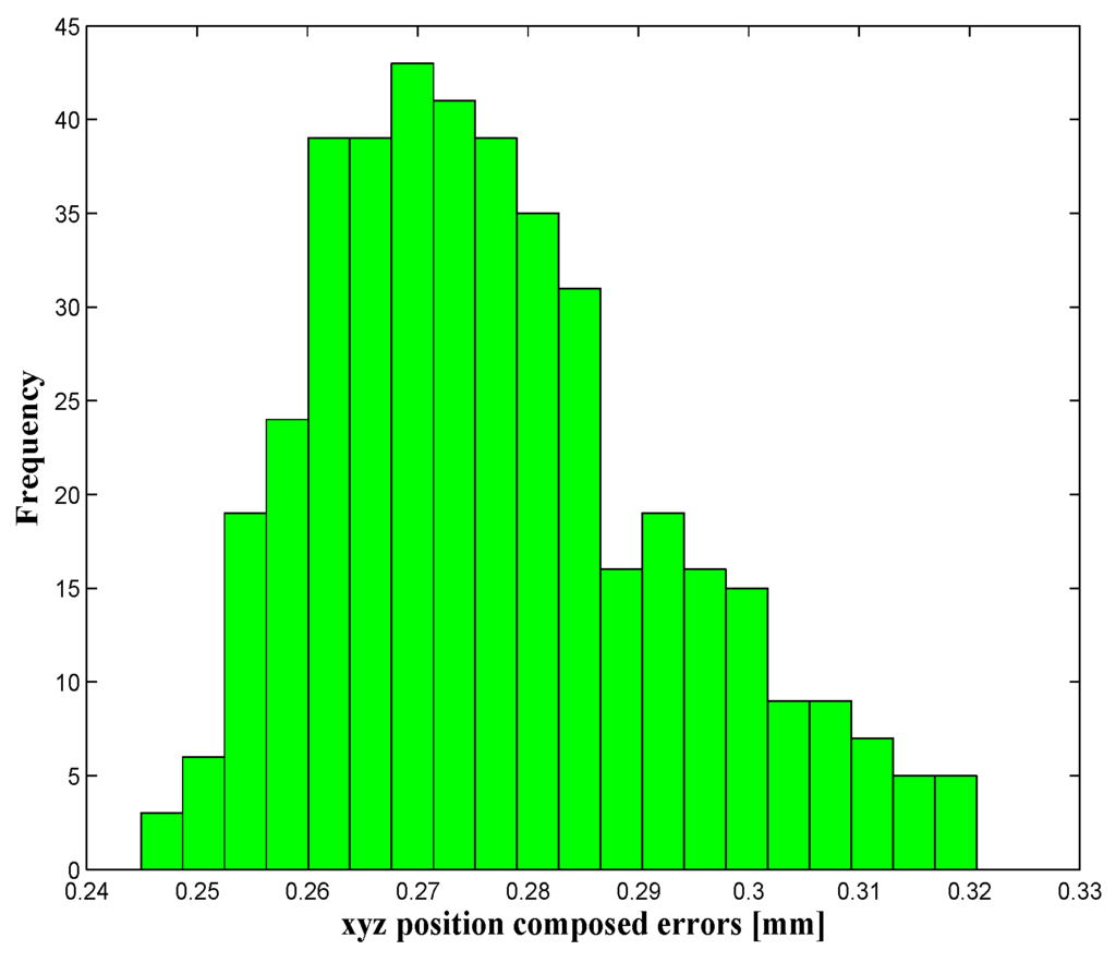
Figure 8.
Position errors in the target workspace after calibration.
A deep analysis of the position errors, for the whole workspace, shows that 0.33% of the evaluated positions have an accuracy lower than 0.2024 mm (mean − 2 × STD), 94.37% are within the range mean ± 2 × STD, and only 5.3% of positions present the poorer accuracy, which is higher than 0.3696 (mean + 2 × STD). The same analysis was achieved for the target workspace, and it shows that 93.0952% of positions have an accuracy within 0.2457 mm and 0.3085 mm (mean ± 2 × STD), and only 6.9048% of positions have errors higher than 0.3085 mm (mean + 2 × STD).
For illustrative purpose, Table 4 shows the accuracy obtained by using each observability index, separately, in the calibration process. Results confirm that O1 is the most appropriate index for calibrating our robot, since it gives the smallest position (and force/torque) errors, after calibration. Moreover, deeper statistical analyses were carried out on the results obtained by the five indices. First we verified whether the data distributions are Gaussian or not, and then used parametric or non-parametric tests accordingly. Therefore a Kolmogorov-Smirnov test (not shown) was achieved, and it showed that all observability indices provide Gaussian distribution. Based on these results, we decided to use parametric analyses (i.e., ANOVA analysis, and t-test).
Initially, an ANOVA analysis, with a probability threshold α = 0.05, is used to confirm the objectivity of comparing the five indices (i.e., confirm that there is actually differences between the use of the five indices). Results show that the F value is significantly higher than the F criteria, which leads to reject the null hypothesis, and therefore conclude that the comparison of results (position accuracy) obtained by using the five indices is meaningful (i.e., results are different, and some indices are better than others).
The ANOVA does not tell where the difference between indices lies. Therefore, an additional test is considered (t-test). The t-test is used to compare each pair of indices. However, the position errors obtained by using O3 and O4 were clearly poorer than results obtained by the other indices (O1, O2, and O5). Thus, only O1, O2, and O5 are considered in the t-Test. The results of this test are shown in Table 5, and they show that the position errors obtained by these three indices are quite different, since the t Stat value is significantly lower than –t_Critical_two-tail, for all pairs of comparisons. Furthermore, to take into account multiple comparison effects, a post-hoc correction is included (Bonferroni correction). As summarized in Table 5, results show that all the t-tests were statistically significant (i.e., there are significant differences between the performances of the observability indices).
Table 5.
Results of the t-test comparing pairs of O1, O2, and O5.
Based on the aboves tests, we conclude that the fives observability indices allow different results, regarding the robot accuracy after calibration. The analysis of the mean and maximum errors (Table 4) shows that the index O1 leads to the best robot accuracy: it gives not only the smallest mean errors, but also the smallest maximum errors. Also, O1 has a small standard deviation, which means that position errors are closely distributed around the mean value.
We recall that in our simulation the used measurement noise was ±1 N. This range of error is an exaggerated error of our wrench sensor (Mini 40, from API). For illustrative propose, we achieved other simulations by considering lower measurement noise (Table 6). Results demonstrate that the accuracy after calibration is much better in case of low measurement errors. However, the impact of these errors can be reduced by:
- -
- Using continuous tracking approach: taking several measurements for each robot calibration configuration (i.e., the same applied force), and then averaging the collected data. Most sensors, and data collection card allow a frequency upper than 100 Hz.
- -
- Calibrating the wrench sensor only in a limited range, in which the sensor will be actually used. This will reduce the measurement uncertainty.
Table 6.
Composite position errors after calibration, inside the target workspace, using different measurement errors.
6. Conclusions
We have presented a self-kinematic calibration approach using a force-torque sensor. With this approach, the position accuracy of a 6-DOF medical robot was significantly improved. The robustness of our calibration model, regarding measurement noise, was confirmed through a simulation study, which also allowed us to conduct an observability analysis in order to identify the most appropriate calibration configurations. The simulation demonstrated that the robot’s position errors were reduced from 12 mm to 0.320 mm for the maximum values, and from 9 mm to 0.277 mm for the mean errors. The calibration method presented in this paper will be tested experimentally in further work.
Acknowledgments
We thank the Canada Research Chairs program for funding this work.
Author Contributions
Ahmed Joubair designed and carried out the calibration study, and wrote the paper; Long Fei Zhao and Pascal Bigras, developed the robot kinematics; Ilian A. Bonev supervised the project.
Conflicts of Interest
The authors declare no conflict of interest.
References
- Beasley, R.A. Medical robots: Current systems and research directions. J. Robot. 2012, 2012. [Google Scholar] [CrossRef]
- Speich, J.E.; Rosen, J. Medical robotics. In Encyclopedia of Biomaterials and Biomedical Engineering; CRC Press: Boca Raton, FL, USA, 2004; pp. 983–993. [Google Scholar]
- Zhao, L.; Yen, A.K.W.; Coulombe, J.; Bigras, P.; Bonev, I.A. Kinematic analyses of a new medical robot for 3D vascular ultrasound examination. Trans. Can. Soc. Mech. Eng. 2013, 38, 227–239. [Google Scholar]
- Vieyres, P.; Poisson, G.; Courrèges, F.; Smith-Guerin, N.; Novales, C.; Arbeille, P. A Tele-Operated Robotic System for Mobile Tele-Echography: The Otelo Project. In M-Health: Emerging Mobile Health Systems; Istepanian, R.S.H., Laxminarayan, S., Pattichis, C.S., Eds.; Springer US: New York, NY, USA, 2006; pp. 461–473. [Google Scholar]
- Pierrot, F.; Dombre, E.; Dégoulange, E.; Urbain, L.; Caron, P.; Gariépy, J.; Mégnien, J.L. Hippocrate: A safe robot arm for medical applications with force feedback. Med. Image Anal. 1999, 3, 285–300. [Google Scholar] [CrossRef]
- Broeders, I.A.M.J.; Ruurda, J. Robotics revolutionizing surgery: The Intuitive Surgical “Da Vinci” system. Ind. Robot Int. J. 2001, 28, 387–392. [Google Scholar] [CrossRef]
- Shimachi, S.; Hirunyanitiwatna, S.; Fujiwara, Y.; Hashimoto, A.; Hakozaki, Y. Adapter for contact force sensing of the da Vinci® robot. Int. J. Med. Robot. Comput. Assist. Surg. 2008, 4, 121–130. [Google Scholar] [CrossRef] [PubMed]
- Schulz, A.P.; Seide, K.; Queitsch, C.; von Haugwitz, A.; Meiners, J.; Kienast, B.; Tarabolsi, M.; Kammal, M.; Jürgens, C. Results of Total Hip Replacement Using the Robodoc Surgical Assistant System: Clinical Outcome and Evaluation of Complications for 97 Procedures. Int. J. Med. Robot. Comput. Assist. Surg. 2007, 3, 301–306. [Google Scholar] [CrossRef] [PubMed]
- Hogan, N.; Krebs, H.I.; Charnnarong, J.; Srikrishna, P.; Sharon, A. MIT-MANUS: A workstation for manual therapy and training. I. In Proceedings of the IEEE International Workshop on Robot and Human Communication, Tokyo, Japan, 1–3 September 1992; pp. 161–165.
- Krebs, H.I.; Ferraro, M.; Buerger, S.P.; Newbery, M.J.; Makiyama, A.; Sandmann, M.; Lynch, D.; Volpe, B.T.; Hogan, N. Rehabilitation robotics: Pilot trial of a spatial extension for MIT-Manus. J. NeuroEng. Rehabil. 2004, 1, 5. [Google Scholar] [CrossRef] [PubMed]
- Galvez, J.A.; Reinkensmeyer, D.J. Robotics for gait training after spinal cord injury. Top. Spinal Cord Inj. Rehabil. 2005, 11, 18–33. [Google Scholar] [CrossRef]
- Otr, O.V.D.N.; Reinders-Messelink, H.A.; Bongers, R.M.; Bouwsema, H.; van der Sluis, C.K. The i-LIMB hand and the DMC plus hand compared: A case report. Prosthet. Orthot. Int. 2010, 34, 216–220. [Google Scholar] [PubMed]
- Low, K. Robot-assisted gait rehabilitation: From exoskeletons to gait systems. In Proceedings of the Defense Science Research Conference and Expo (DSR), Singapore, 3–5 August 2011; pp. 1–10.
- Joubair, A.; Slamani, M.; Bonev, I.A. Kinematic calibration of a 3-DOF planar parallel robot. Ind. Robot 2012, 39, 392–400. [Google Scholar] [CrossRef]
- Joubair, A.; Slamani, M.; Bonev, I.A. Kinematic calibration of a five-bar planar parallel robot using all working modes. Robot. Comput. Integr. Manuf. 2013, 29, 15–25. [Google Scholar] [CrossRef]
- Joubair, A.; Nubiola, A.; Bonev, I.A. Calibration efficiency analysis based on five observability indices and two calibration models for a six-axis industrial robot. SAE Int. J. Aerosp. 2013, 6, 161–168. [Google Scholar] [CrossRef]
- Nubiola, A.; Slamani, M.; Joubair, A.; Bonev, A.I. Comparison of two calibration methods for a small industrial robot based on an optical CMM and a laser tracker. Robotica 2013, 32, 447–466. [Google Scholar] [CrossRef]
- Joubair, A.; Bonev, I.A. Absolute accuracy analysis and improvement of a hybrid 6-DOF medical robot. Ind. Robot 2015, 42, 44–53. [Google Scholar] [CrossRef]
- Kim, H.S. Kinematic calibration of a Cartesian parallel manipulator. Int. J. Control Autom. Syst. 2005, 3, 453–460. [Google Scholar]
- Huang, T.; Hong, Z.Y.; Mei, J.P.; Chetwynd, D.G. Kinematic calibration of the 3-DOF module of a 5-DOF reconfigurable hybrid robot using a double-ball-bar system. In Proceedings of the IEEE/RSJ International Conference on Intelligent Robots and Systems, Beijing, China, 9–15 October 2006; pp. 508–512.
- Joubair, A.; Bonev, I.A. Kinematic calibration of a six-axis serial robot using distance and sphere constraints. Int. J. Adv. Manuf. Technol. 2014, 77, 515–523. [Google Scholar] [CrossRef]
- Joubair, A.; Bonev, I.A. Non-kinematic calibration of a six-axis serial robot using planar constraints. Precis. Eng. 2015, 40, 325–333. [Google Scholar] [CrossRef]
- Gabiccini, M.; Stillfried, G.; Marino, H.; Bianchi, M. A data-driven kinematic model of the human hand with soft-tissue artifact compensation mechanism for grasp synergy analysis. In Proceedings of the IEEE/RSJ International Conference on Intelligent Robots and Systems—IROS, Tokyo, Japan, 3–7 November 2013.
- Mitchell, T.J. An algorithm for the construction of D-optimal experimental designs. Technometrics 1974, 42, 203–210. [Google Scholar]
- Sun, Y.; Hollerbach, J. Observability index selection for robot calibration. In Proceedings of the IEEE International Conference on Robotics and Automation, Pasadena, CA, USA, 19–23 May 2008.
- Joubair, A.; Bonev, I.A. Comparison of the efficiency of five observability indices for robot calibration. Mech. Mach. Theory 2013, 70, 254–265. [Google Scholar] [CrossRef]
© 2016 by the authors; licensee MDPI, Basel, Switzerland. This article is an open access article distributed under the terms and conditions of the Creative Commons Attribution (CC-BY) license (http://creativecommons.org/licenses/by/4.0/).