
Coupled Integration of CSAC, MIMU, and GNSS for Improved PNT Performance


Abstract
:1. Introduction
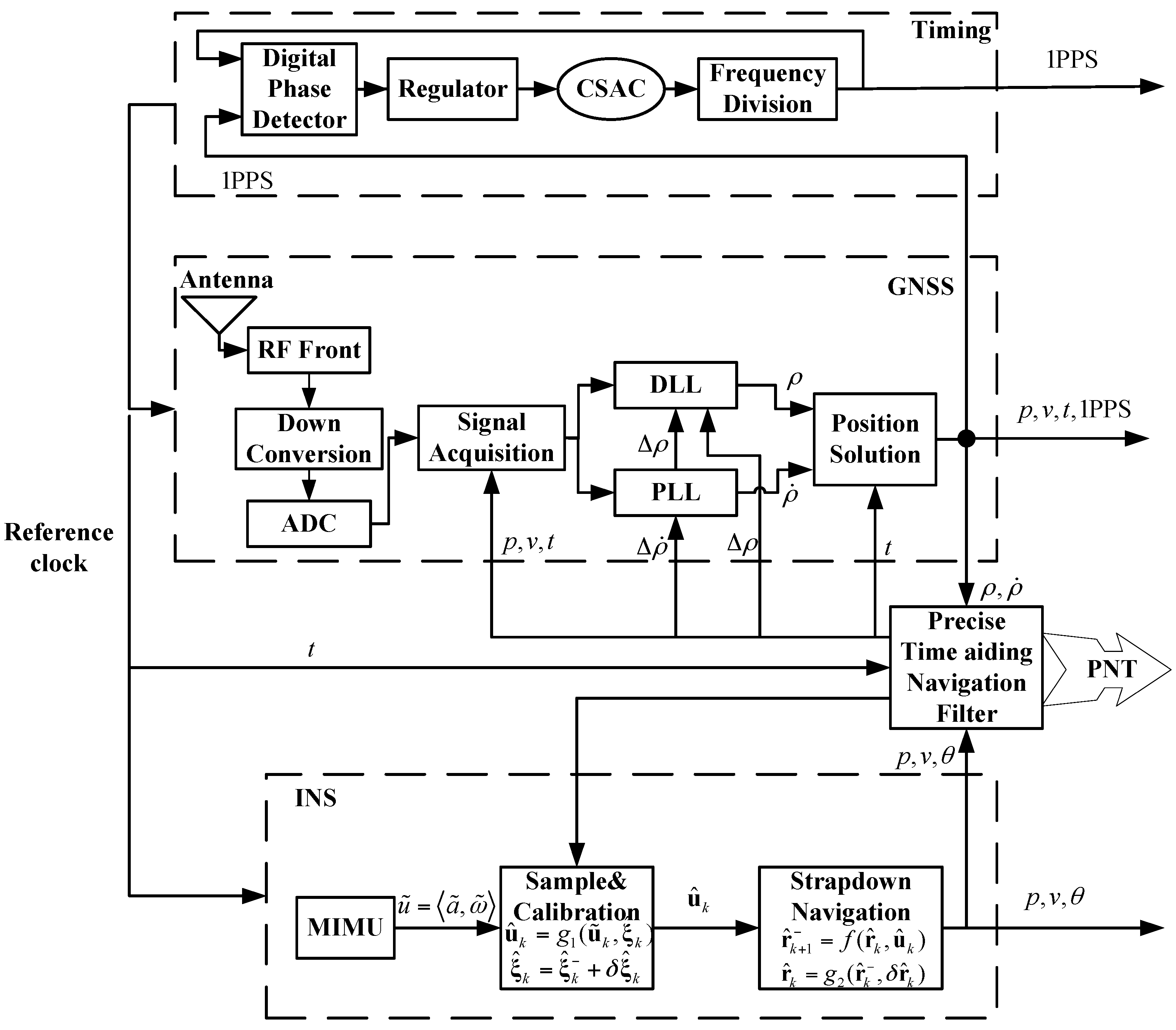
2. Architecture of Coupled Integration
3. Mathematical Model of Precise Time-Aiding Navigation Filter
3.1. Integration State Model
3.2. Integration Observation Model
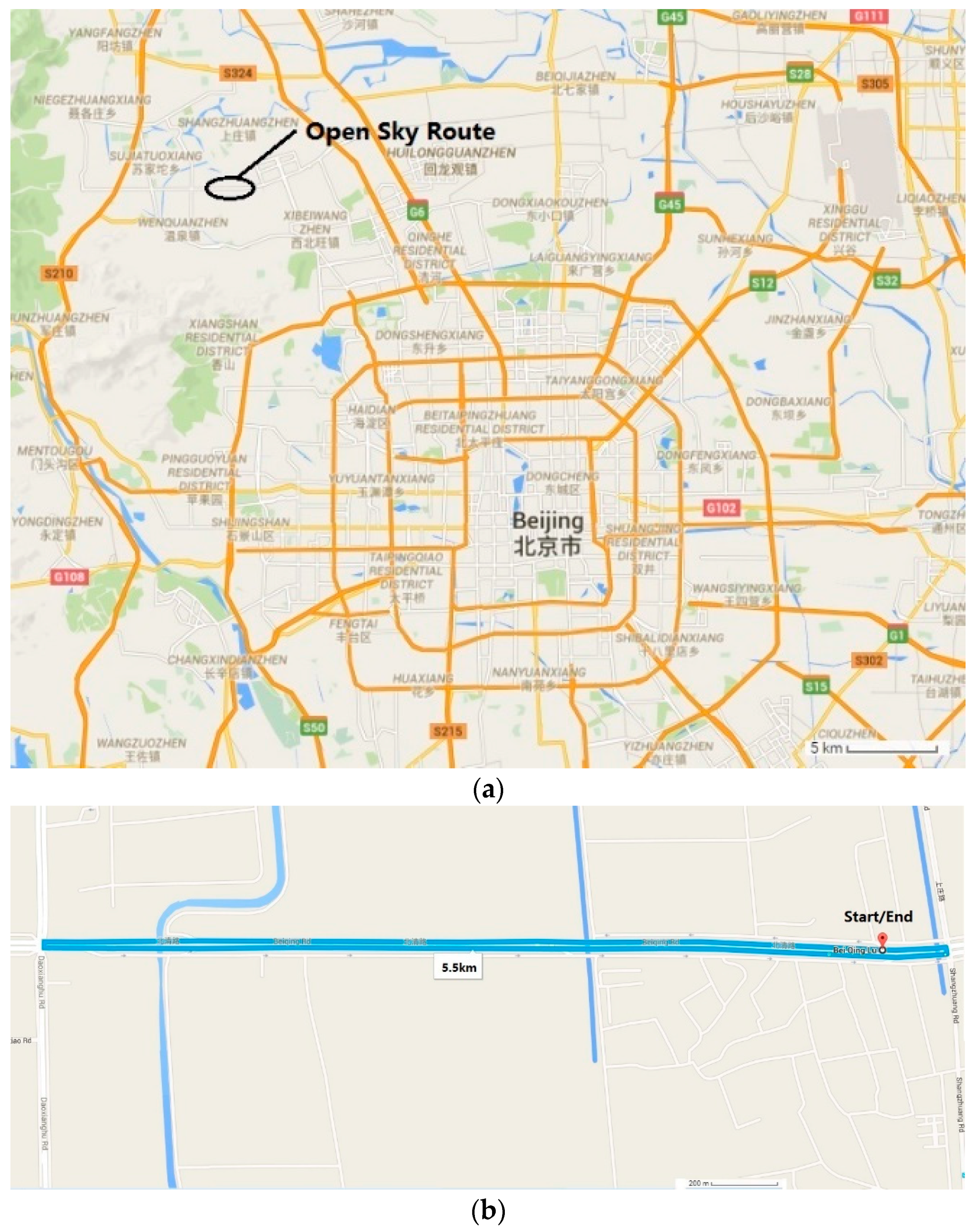
4. Field Vehicle Experiments
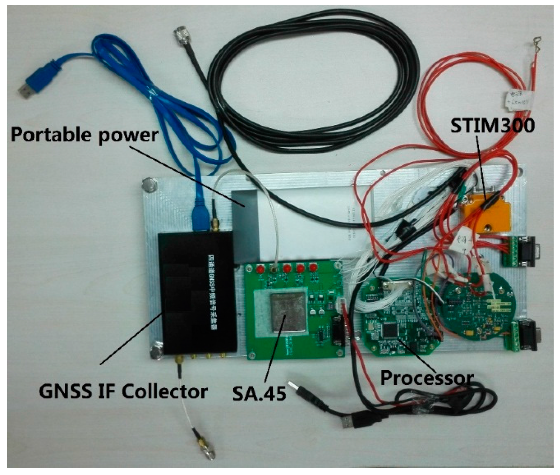
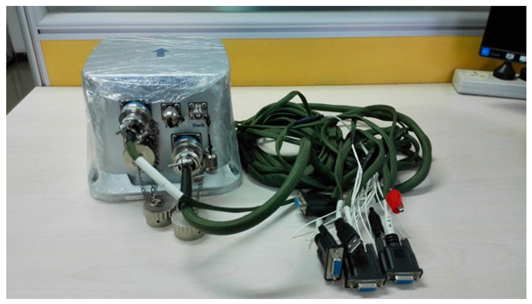
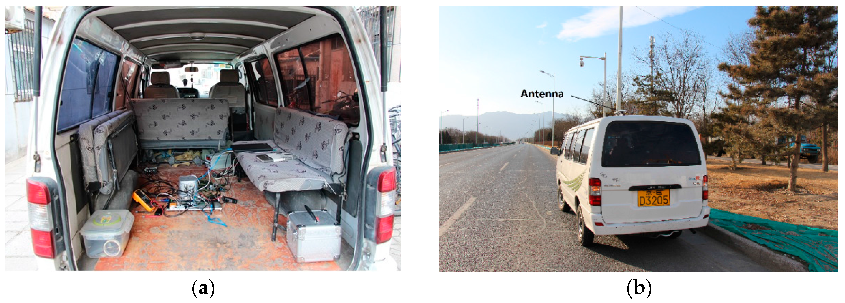
4.1. Experimental Setup
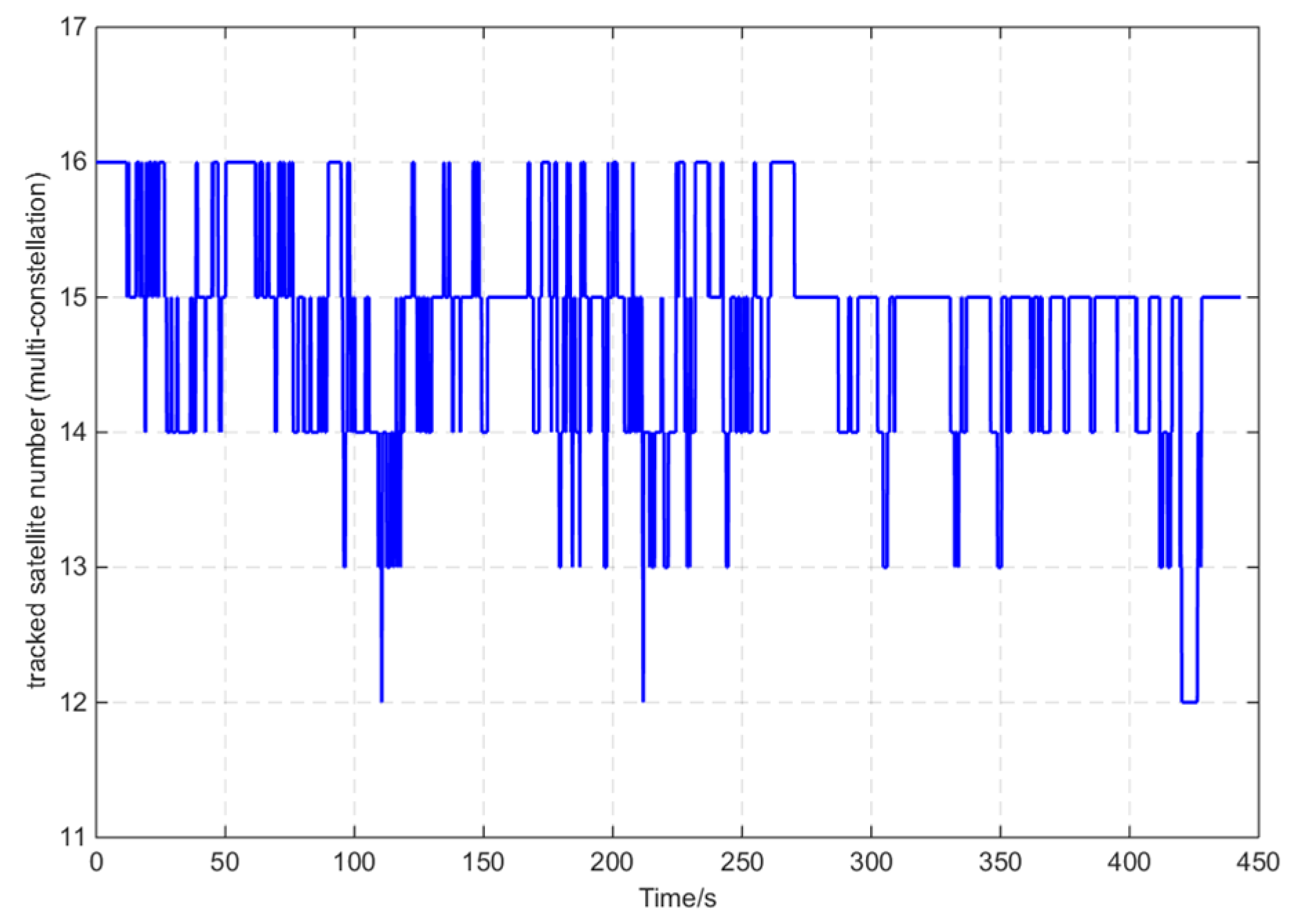
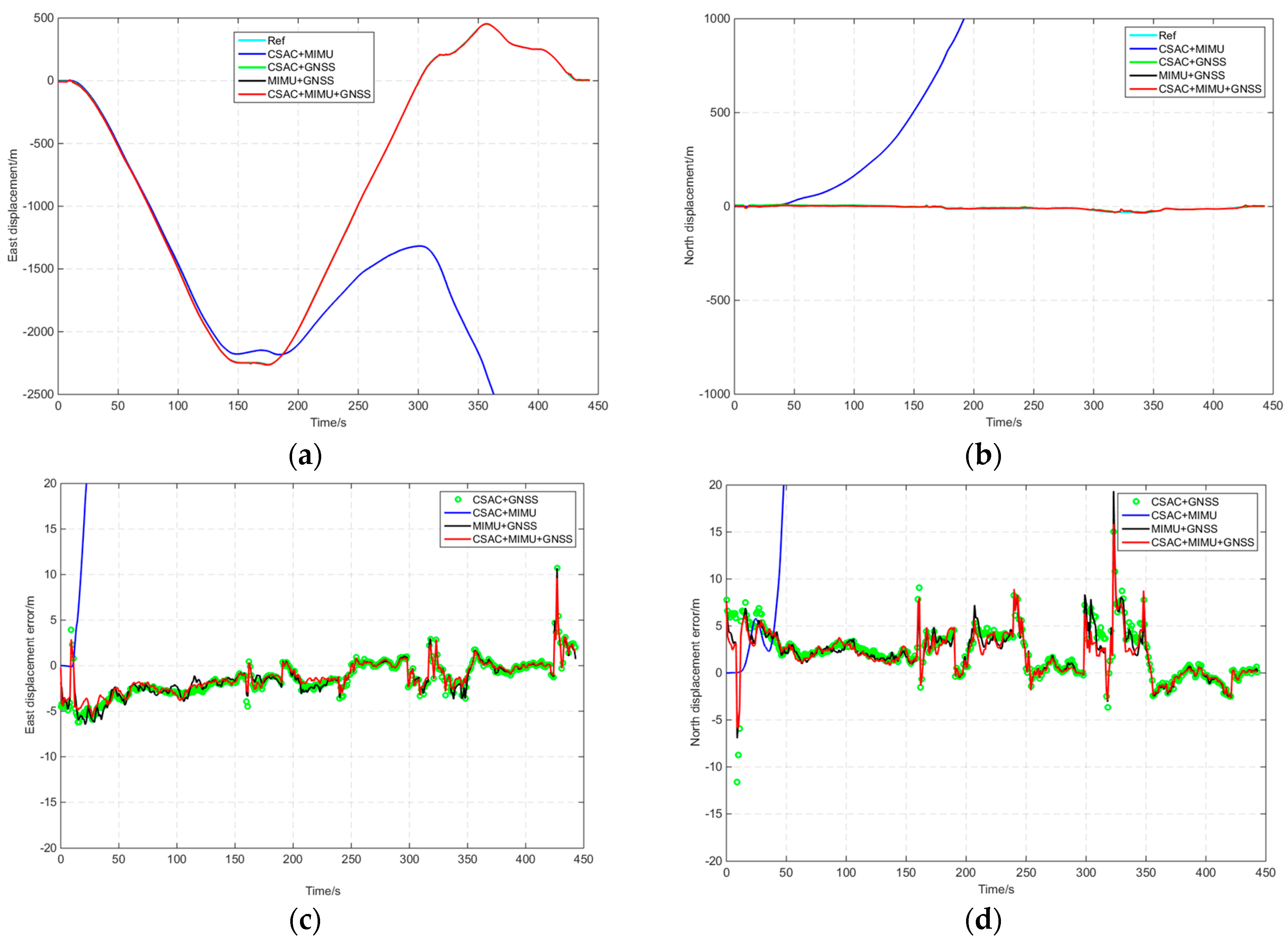
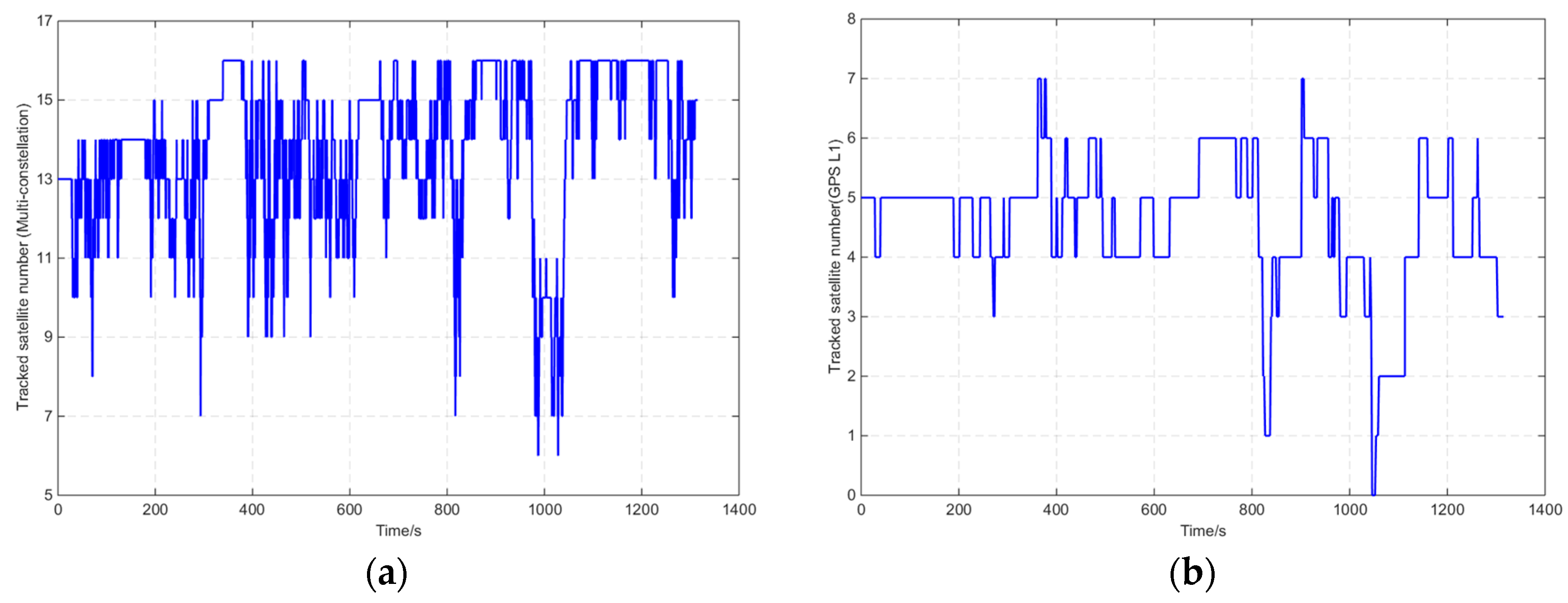
4.2. Open-Sky Route
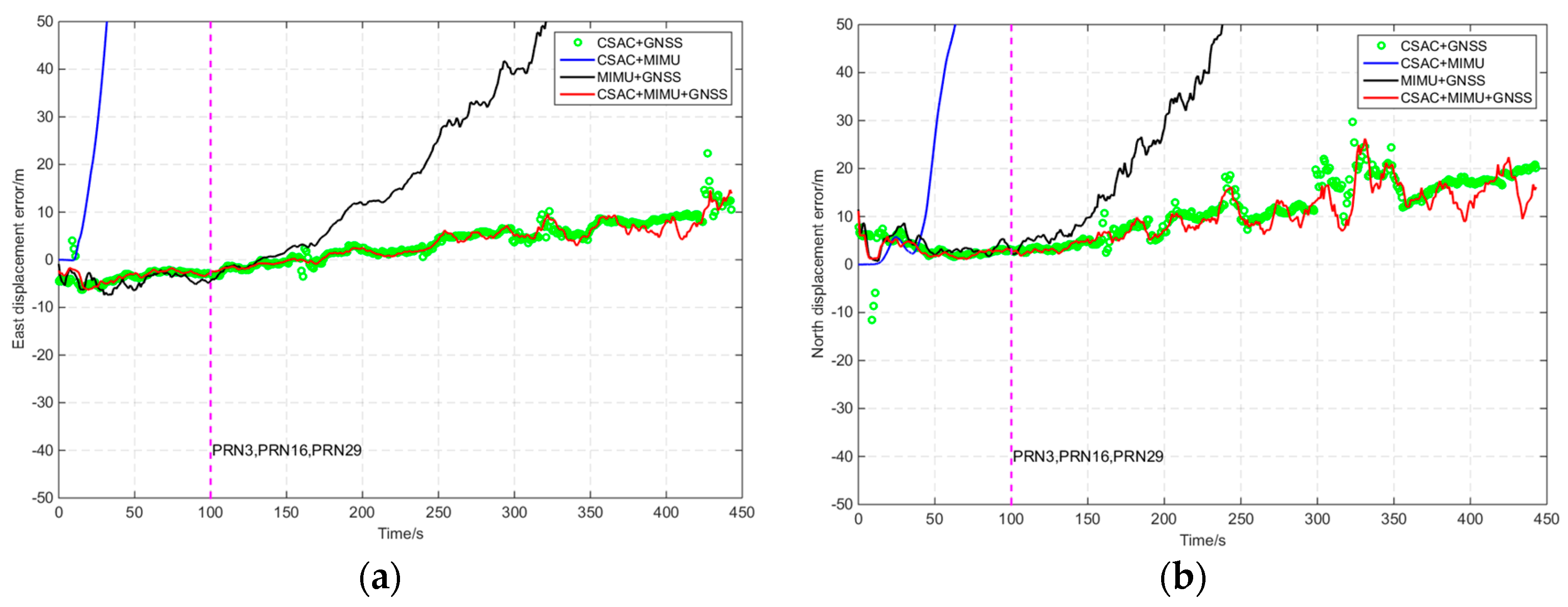
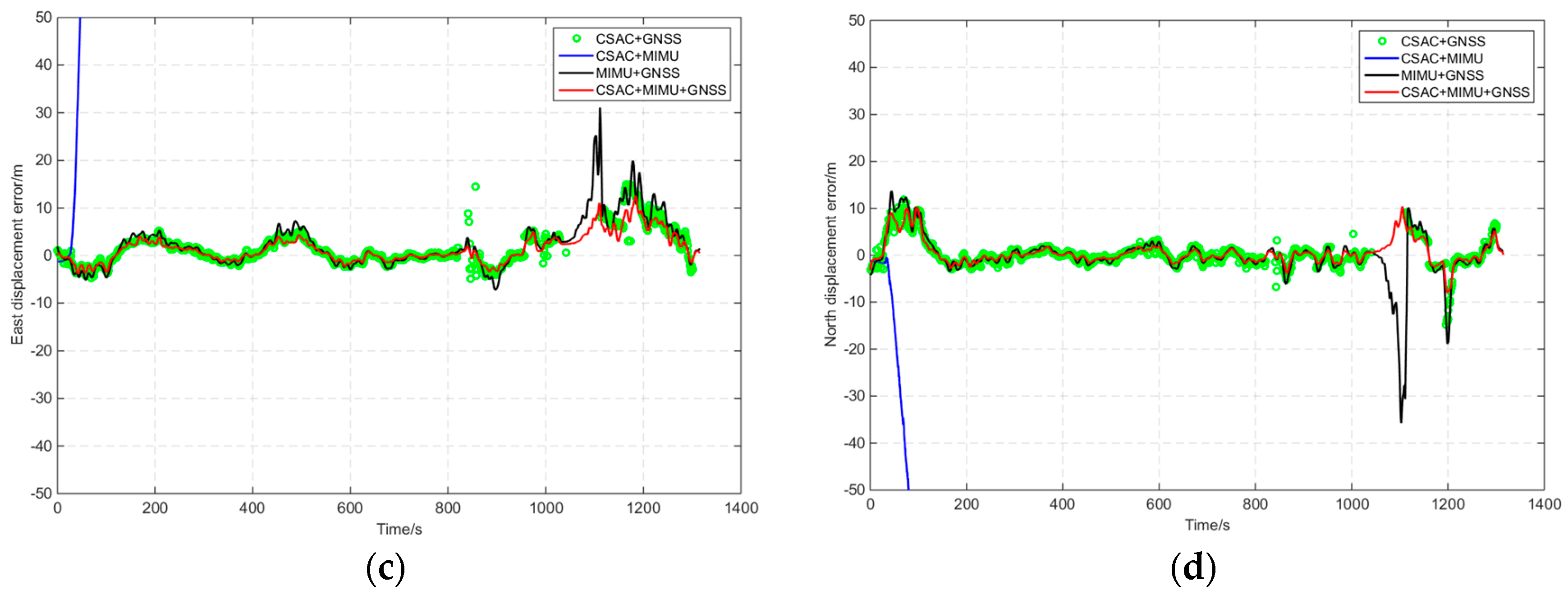
4.3. Harsh Route
5. Conclusions
Acknowledgments
Author Contributions
Conflicts of Interest
Appendix A

References
- Kaplan, E.D.; Hegarty, C.J. Understanding GPS: Principles and Application, 2nd ed.; Artech House: Norwood, MA, USA, 2006. [Google Scholar]
- McNeff, J. Changing the Game Changer—The Way Ahead for Military PNT. Inside GNSS 2010, 5, 44–51. [Google Scholar]
- Alexander, K. US space based PNT policy and GPS modernization. In Proceedings of the United Nations/Zambia/ESA Regional Workshop on the Applications of Global Navigation Satellite System Technologies in Sub-Saharan Africa, Lusaka, Zambia, 26 June 2006.
- Groves, P.D. The PNT Boom: Future Trends in Integrated Navigation. Inside GNSS 2013, 8, 44–49. [Google Scholar]
- Britting, K.R. Inertial Navigation Systems Analysis; Artech House: Norwood, MA, USA, 2010. [Google Scholar]
- Titterton, D.H.; Weston, J.L. Strapdown Inertial Navigation Technology; Institution of Electrical Engineers: Stevenage, UK, 2004. [Google Scholar]
- Woodman, O.J. An Introduction to Inertial Navigation; Technical Report UCAMCL-TR-696 for Computer Laboratory; University of Cambridge: Cambridge, UK, 2007. [Google Scholar]
- Shibata, M. Error analysis strapdown inertial navigation using quaternions. J. Guid. Control Dyn. 1986, 9, 379–381. [Google Scholar] [CrossRef]
- Groves, P.D. Principles of GNSS, Inertial, and Multi-Sensor Integrated Navigation Systems; Artech House: Norwood, MA, USA, 2013. [Google Scholar]
- Cong, L.; Li, E.; Qin, H.; Ling, K.V.; Xue, R. A Performance Improvement Method for Low-Cost Land Vehicle GPS/MEMS-INS Attitude Determination. Sensors 2015, 15, 5722–5746. [Google Scholar] [CrossRef] [PubMed]
- Han, H.; Wang, J.; Wang, J.; Tan, X. Performance Analysis on Carrier Phase-Based Tightly-Coupled GPS/BDS/INS Integration in GNSS Degraded and Denied Environments. Sensors 2015, 15, 8685–8711. [Google Scholar] [CrossRef] [PubMed]
- Yang, L.; Li, Y.; Wu, Y.; Rizos, C. An enhanced MEMS-INS/GNSS integrated system with fault detection and exclusion capability for land vehicle navigation in urban areas. GPS Solut. 2014, 18, 593–603. [Google Scholar] [CrossRef]
- Fan, C.; Hu, X.; He, X.; Tang, K.; Luo, B. Observability Analysis of a MEMS INS/GPS Integration System with Gyroscope G-Sensitivity Errors. Sensors 2014, 14, 16003–16016. [Google Scholar] [CrossRef] [PubMed]
- Zhao, L.; Qiu, H.; Feng, Y. Study of Robust Filtering Application in Loosely Coupled INS/GPS System. Math. Probl. Eng. 2014, 2014. [Google Scholar] [CrossRef]
- Chang, G. Loosely Coupled INS/GPS Integration with Constant Lever Arm using Marginal Unscented Kalman Filter. J. Navig. 2014, 67, 419–436. [Google Scholar] [CrossRef]
- Tawk, Y.; Tomé, P.; Botteron, C.; Stebler, Y.; Farine, P.-A. Implementation and Performance of a GPS/INS Tightly Coupled Assisted PLL Architecture Using MEMS Inertial Sensors. Sensors 2014, 14, 3768–3796. [Google Scholar] [CrossRef] [PubMed]
- Rabbou, M.A.; El-Rabbany, A. Tightly coupled integration of GPS precise point positioning and MEMS-based inertial systems. GPS Solut. 2014, 19, 601–609. [Google Scholar] [CrossRef]
- Ban, Y.; Niu, X.; Zhang, T.; Zhang, Q.; Guo, W.; Zhang, H. Low-end MEMS IMU can contribute in GPS/INS deep integration. In Proceedings of the IEEE/ION Position, Location and Navigation Symposium-PLANS, Monterey, CA, USA, 5–8 May 2014.
- Yang, J.; Shan, X. Satellite Timing Principle and Application; National Defense Industry Press: Beijing, China, 2013; pp. 130–133. [Google Scholar]
- Lutwak, R. Chip-Scale Atomic Clock (Briefing Charts); Symmetricom-Technology Realization Center: Beverly, MA, USA, 2007. [Google Scholar]
- SA.3Xm. Timing & Synchronization Systems. Available online: http://www.symmetricom.com/products/frequency-references/rubidium-frequency-standard (accessed on 9 March 2016).
- Sturza, M.A. GPS navigation using three satellites and a precise clock. Navigation 1983, 30, 146–156. [Google Scholar] [CrossRef]
- Van Graas, F.; Braasch, M. GPS interferometric attitude and heading determination: Initial flight test results. Navigation 1992, 38, 297–316. [Google Scholar] [CrossRef]
- Misra, P.; Pratt, M.; Muchnik, R.; Manganis, B. A general RAIM algorithm based on receiver clock Autonomous Integrity Monitoring. In Proceedings of the 8th International Technical Meeting of the Satellite Division of the Institute of Navigation, Palm Springs, CA, USA, 12–15 September 1995; pp. 1941–1948.
- Kline, P.A. Atomic Clock Augmentation for Receivers Using the Global Positioning System; Virginia Polytechnic Institute and State University: Blacksburg, VA, USA, 1997. [Google Scholar]
- Zhang, Z. Impact of Rubidium Clock Aiding on GPS Augmented Vehicular Navigation; University of Calgary: Calgary, AB, Canada, 1997. [Google Scholar]
- Bednarz, S.G. Adaptive Modeling of GPS Receiver Clock for Integrity Monitoring during Precision Approaches; Massachusetts Institute of Technology: Cambridge, MA, USA, 2004. [Google Scholar]
- Ma, L.; You, Z.; Li, B.; Zhou, B.; Han, R. Deep Coupled Integration of CSAC and GNSS for Robust PNT. Sensors 2015, 15, 23050–23070. [Google Scholar] [CrossRef] [PubMed]


| Number | Subsystem Status | Mode | ||
|---|---|---|---|---|
| CSAC | MIMU | GNSS | ||
| 1 | √ | √ | √ | Coupled integration |
| 2 | × | √ | √ | MIMU/GNSS tightly coupled integration |
| 3 | √ | × | √ | CSAC/GNSS coupled integration |
| 4 | √ | √ | × | Inertial navigation |
| Sensor | Parameter | Value | |
|---|---|---|---|
| CSAC | Output | 10 MHz (3.3V CMOS) 1 PPS | |
| Accuracy | <±5 × 10⁻¹¹ | ||
| Short term frequency stability | @1 s | 1.5 × 10⁻¹⁰ | |
| @10 s | 5 × 10⁻¹¹ | ||
| @100 s | 1.5 × 10⁻¹¹ | ||
| Phase noise (dbc/Hz) | @1 Hz | <−55 | |
| @10 Hz | <−78 | ||
| @100 Hz | <−113 | ||
| @1 KHz | <−128 | ||
| @10 KHz | <−135 | ||
| Power consumption | <120 mW | ||
| Size | 40.6 mm × 35.5 mm × 11.4 mm | ||
| MIMU | Gyroscope | Range | ±400°/h |
| Bias stability (Allan, ) | 0.5°/h | ||
| Bias stability (Average time, 10 s) | 6°/h | ||
| Angle random walk | 0.15°/√h | ||
| Accelerometer | Range | g | |
| Bias stability (Allan, ) | 50 μg | ||
| Bias stability (Average time, 10 s) | 70 μg | ||
| Velocity random walk | 0.06 m/s/√h | ||
| Power consumption | 1.5 W | ||
| Weight | 55 g | ||
| Size | 38.6 mm × 44.8 mm × 21.5 mm | ||
| GPS L1 IF collector | Chip type | MAX2769 | |
| Signal | GPS L1 | ||
| Intermediate frequency | 4.02 MHz | ||
| Clock frequency | 10 MHz | ||
| Sample rate | 20 MHz | ||
| Sample digits | 8 bit | ||
| Parameter | Value | ||
|---|---|---|---|
| Horizontal positioning accuracy | Single point positioning L1/L2 | 1.2 m () | |
| Differential Global Positioning System (DGPS) | 0.4 m () | ||
| RTK | 2 cm () | ||
| Altitude accuracy | 0.02° | ||
| Velocity accuracy | 0.02 m/s () | ||
| Gyroscope | Type | Close-loop optical fiber | |
| Range | ±300 °/s | ||
| Stability (Average time, 10 s) | <0.3 °/h | ||
| Accelerometer | Type | Quartz | |
| Range | ±10 g | ||
| Stability (Average time, 10 s) | 20 μg | ||
| Power consumption | 20 W | ||
| Size | 189 mm × 169 mm × 133 mm | ||
| Parameter | Value | |
|---|---|---|
| Output frequency | 10 MHz | |
| Frequency stability | 5 × 10⁻⁸ | |
| Phase noise | @10 Hz | <−95 |
| @100 Hz | <−125 | |
| @1 KHz | <−135 | |
| @10 KHz | <−150 | |
| Power consumption | 3 W | |
| Mode | East | North | Horizontal | |||
|---|---|---|---|---|---|---|
| Mean/m | Std/m | Mean/m | Std/m | Mean/m | Std/m | |
| CSAC+GNSS | −1.44 | 1.95 | 2.25 | 2.66 | 3.50 | 2.40 |
| CSAC+MIMU | >500 | >500 | >500 | |||
| MIMU+GNSS | −2.41 | 2.76 | 3.27 | 3.17 | 3.85 | 2.58 |
| CSAC+MIMU+GNSS | −1.24 | 1.74 | 1.95 | 2.40 | 3.04 | 2.15 |
| Mode | East | North | Horizontal | |||
|---|---|---|---|---|---|---|
| Mean/m | Std/m | Mean/m | Std/m | Mean/m | Std/m | |
| CSAC+GNSS | 2.50 | 4.91 | 10.07 | 6.41 | 11.38 | 6.59 |
| CSAC+MIMU | >500 | >500 | >500 | |||
| MIMU+GNSS | >100 | >100 | >100 | |||
| CSAC+MIMU+GNSS | 2.02 | 4.16 | 8.45 | 2.02 | 9.76 | 8.45 |
| Mode | East | North | Horizontal | Positioning Probability | |||
|---|---|---|---|---|---|---|---|
| Mean/m | Std/m | Mean/m | Std/m | Mean/m | Std/m | ||
| CSAC+GNSS | 1.46 | 3.53 | 0.31 | 2.92 | 3.63 | 3.17 | 89% |
| CSAC+MIMU | >500 | >500 | >500 | Failed | |||
| MIMU+GNSS | 2.55 | 4.92 | −1.18 | 5.10 | 5.37 | 5.43 | 100% |
| CSAC+MIMU+GNSS | 1.83 | 3.89 | 0.95 | 3.59 | 4.10 | 3.79 | 100% |
© 2016 by the authors; licensee MDPI, Basel, Switzerland. This article is an open access article distributed under the terms and conditions of the Creative Commons Attribution (CC-BY) license (http://creativecommons.org/licenses/by/4.0/).
Share and Cite
Ma, L.; You, Z.; Liu, T.; Shi, S. Coupled Integration of CSAC, MIMU, and GNSS for Improved PNT Performance. Sensors 2016, 16, 682. https://doi.org/10.3390/s16050682
Ma L, You Z, Liu T, Shi S. Coupled Integration of CSAC, MIMU, and GNSS for Improved PNT Performance. Sensors. 2016; 16(5):682. https://doi.org/10.3390/s16050682
Chicago/Turabian StyleMa, Lin, Zheng You, Tianyi Liu, and Shuai Shi. 2016. "Coupled Integration of CSAC, MIMU, and GNSS for Improved PNT Performance" Sensors 16, no. 5: 682. https://doi.org/10.3390/s16050682
APA StyleMa, L., You, Z., Liu, T., & Shi, S. (2016). Coupled Integration of CSAC, MIMU, and GNSS for Improved PNT Performance. Sensors, 16(5), 682. https://doi.org/10.3390/s16050682