
Multibeam 3D Underwater SLAM with Probabilistic Registration


Abstract
:1. Introduction
2. Submap Creation
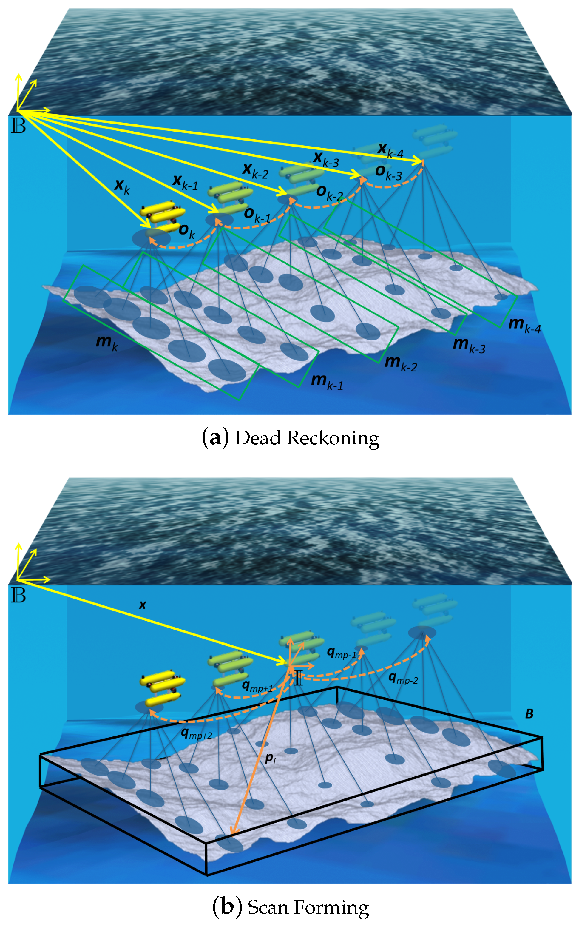
2.1. Dead Reckoning
2.2. Submap Forming
- Minimum size: A minimum size is defined to avoid handling a large number of tiny patches augmenting unnecessarily the length of the SLAM state vector and reducing the overlapping.
- Maximum size: The maximum size is bounded to avoid handling huge patches with a high uncertainty in the surface points due to the accumulated dead reckoning error.
- Normal occupancy: The surface relief is analyzed to determine when the patch is rich enough to be successfully matched. The procedure basically consists in finding surface normals for each point on the cloud and representing their parametrization on a histogram. If the histogram is sufficiently occupied, the submap is closed.
3. Registration Algorithm
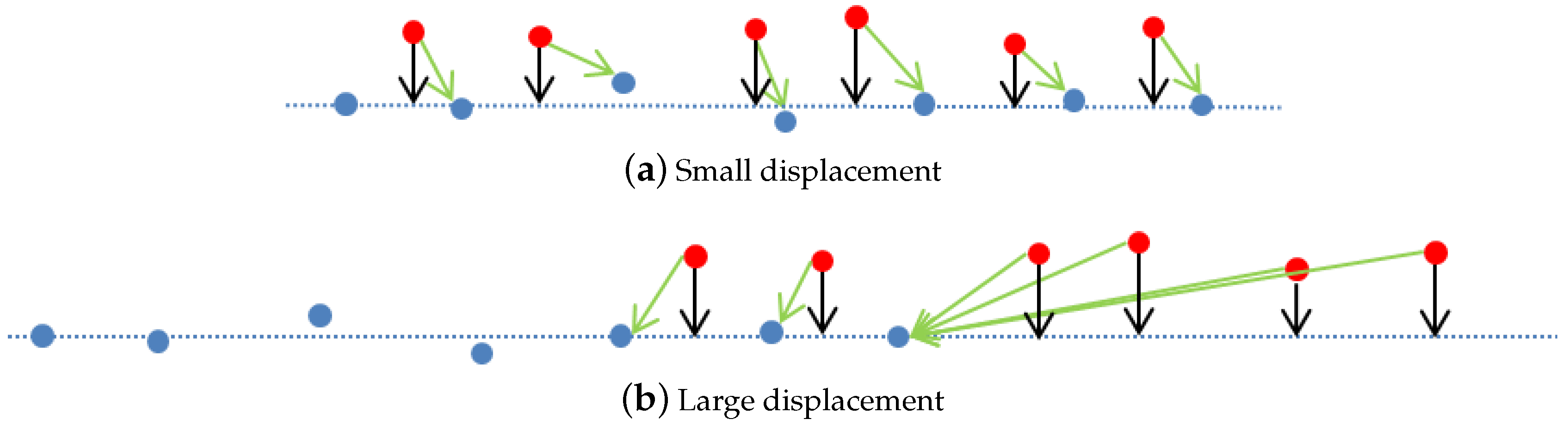
3.1. Point-to-Point Association
3.2. Point-to-Plane Association
3.3. Minimization
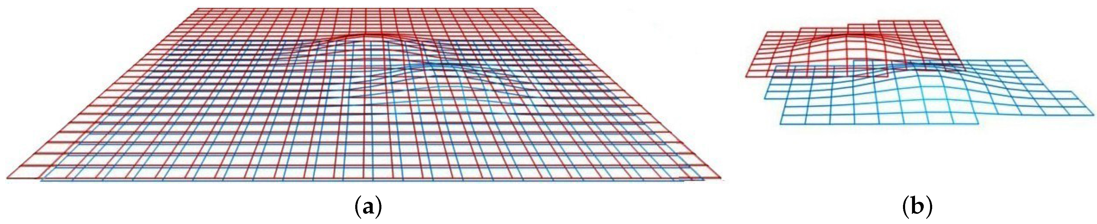
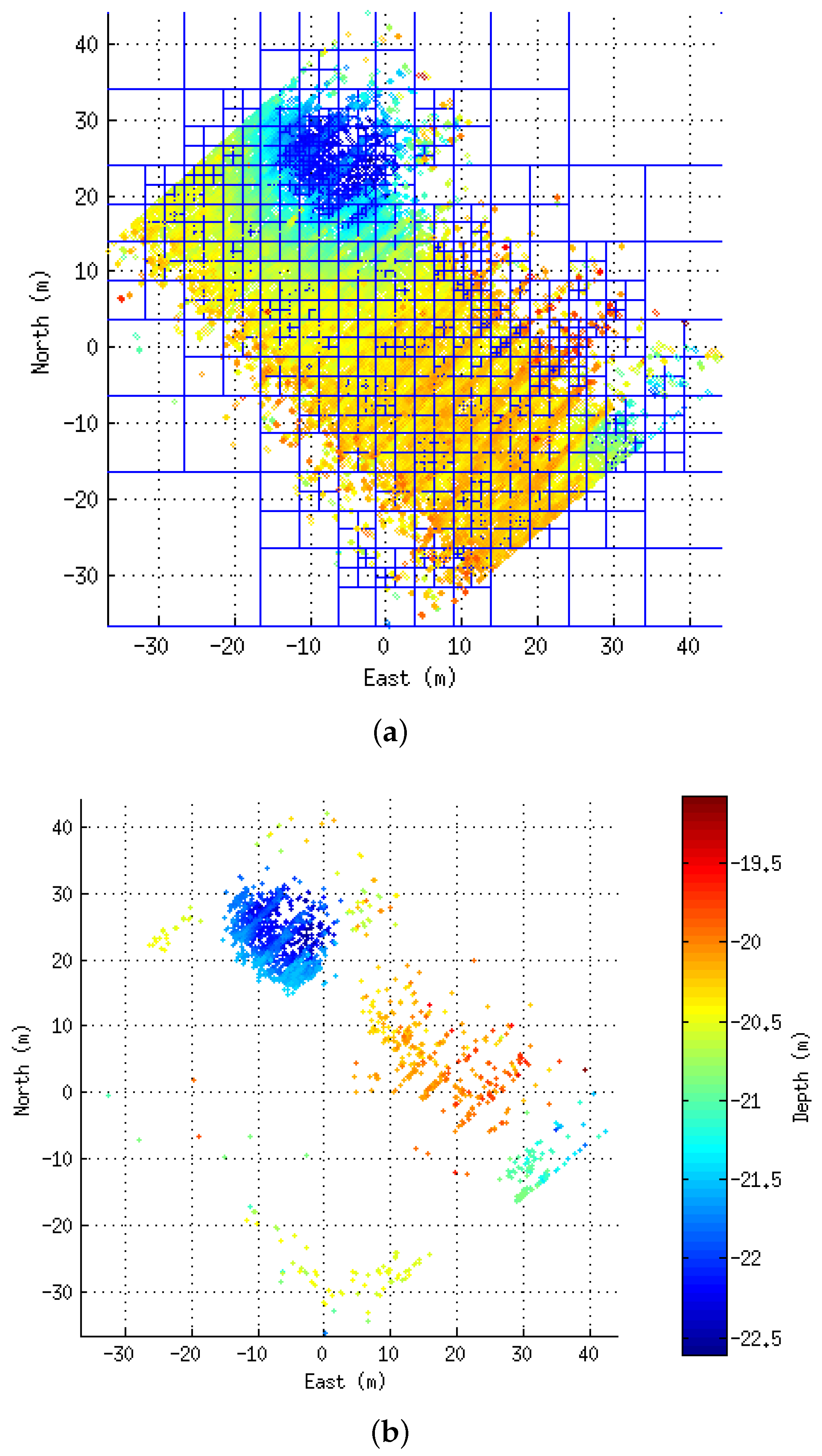
3.4. Submap Simplification
3.5. Association in Linear Time
4. SLAM Algorithm
4.1. Prediction and State Augmentation
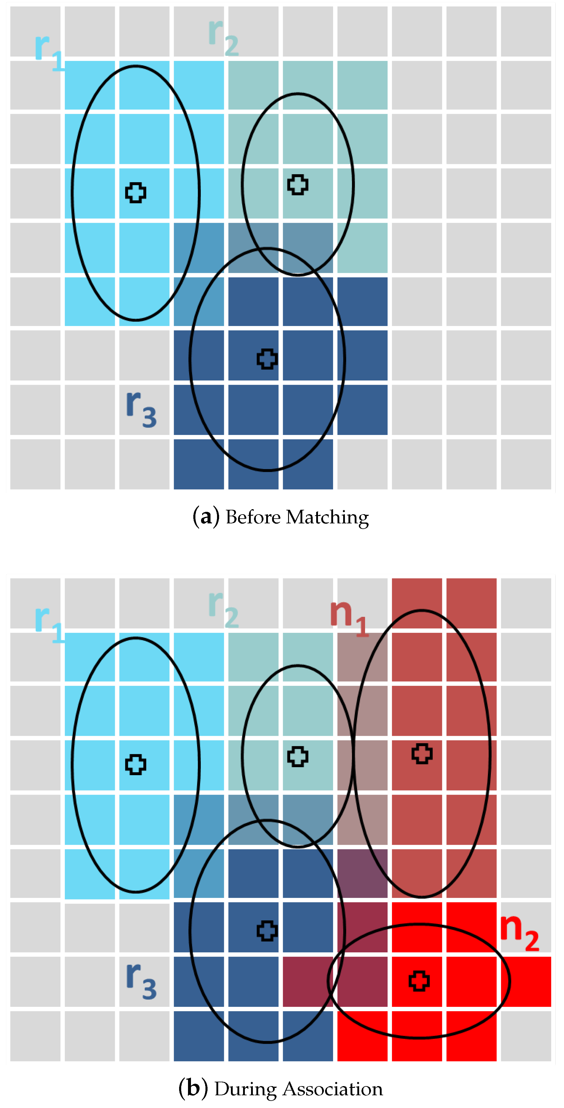
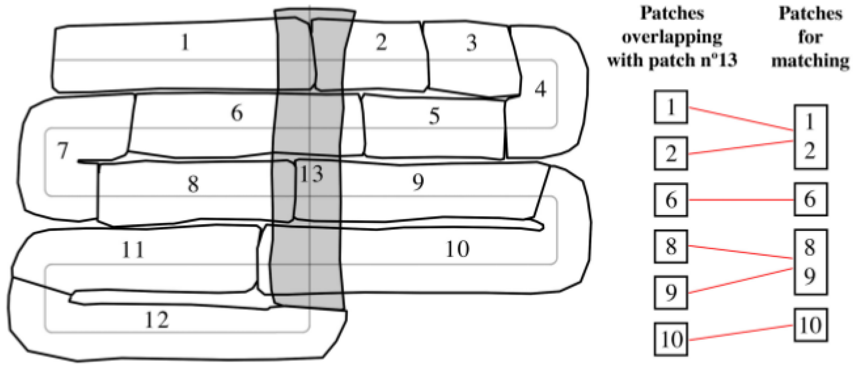
4.2. Matching Strategy
4.3. Scan Matching
4.4. State Update
5. Experiments and Results
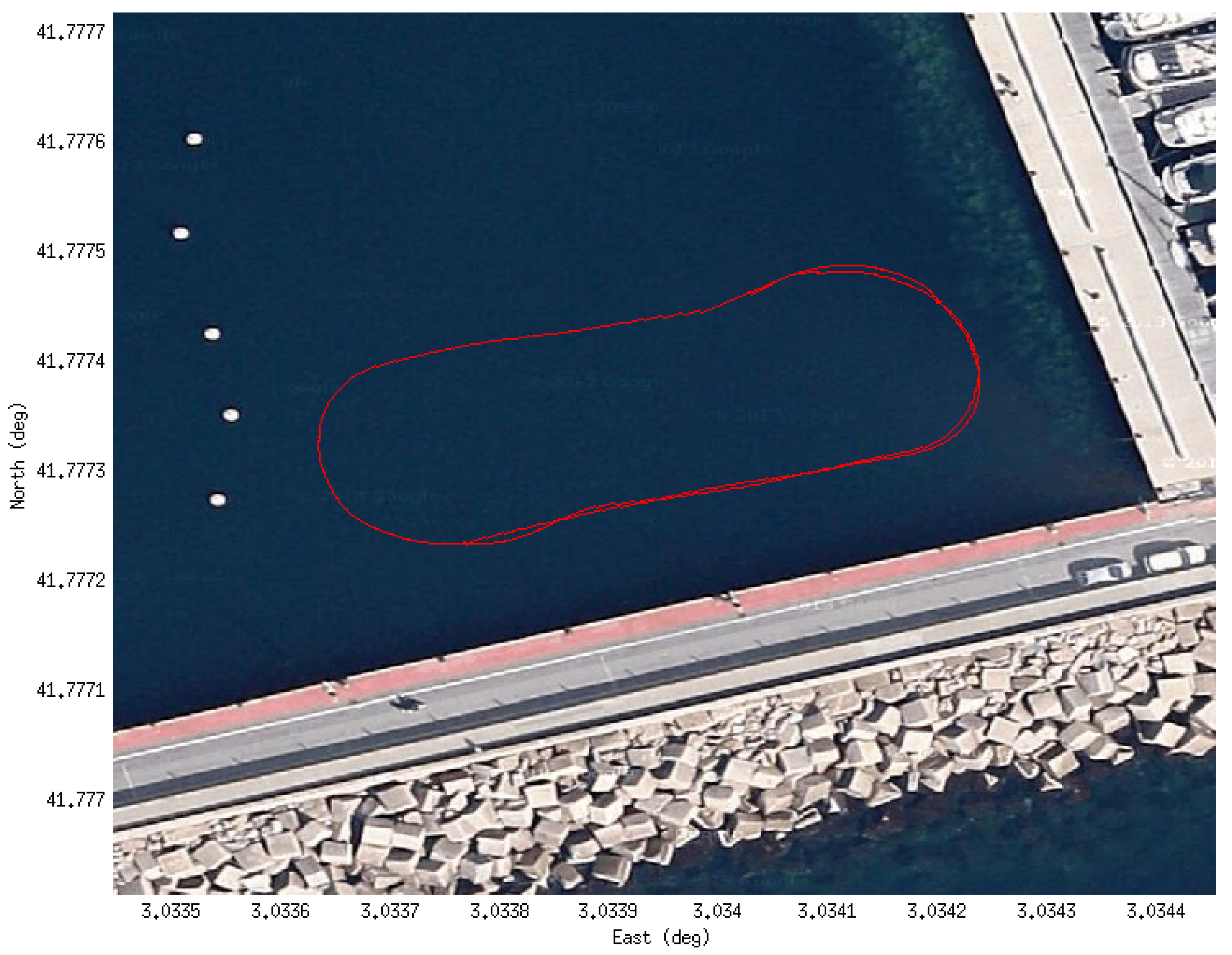
5.1. Bathymetric Survey
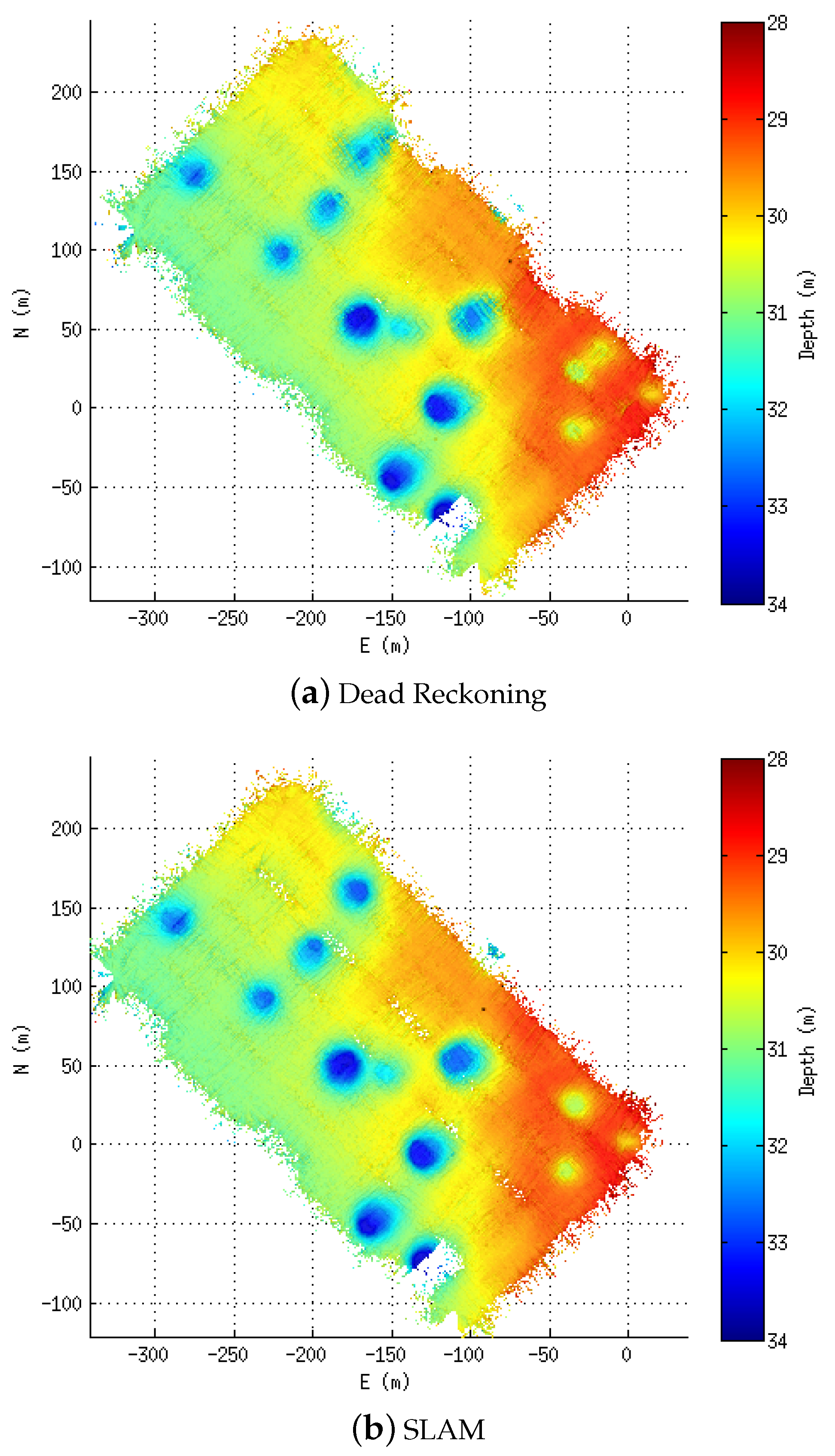
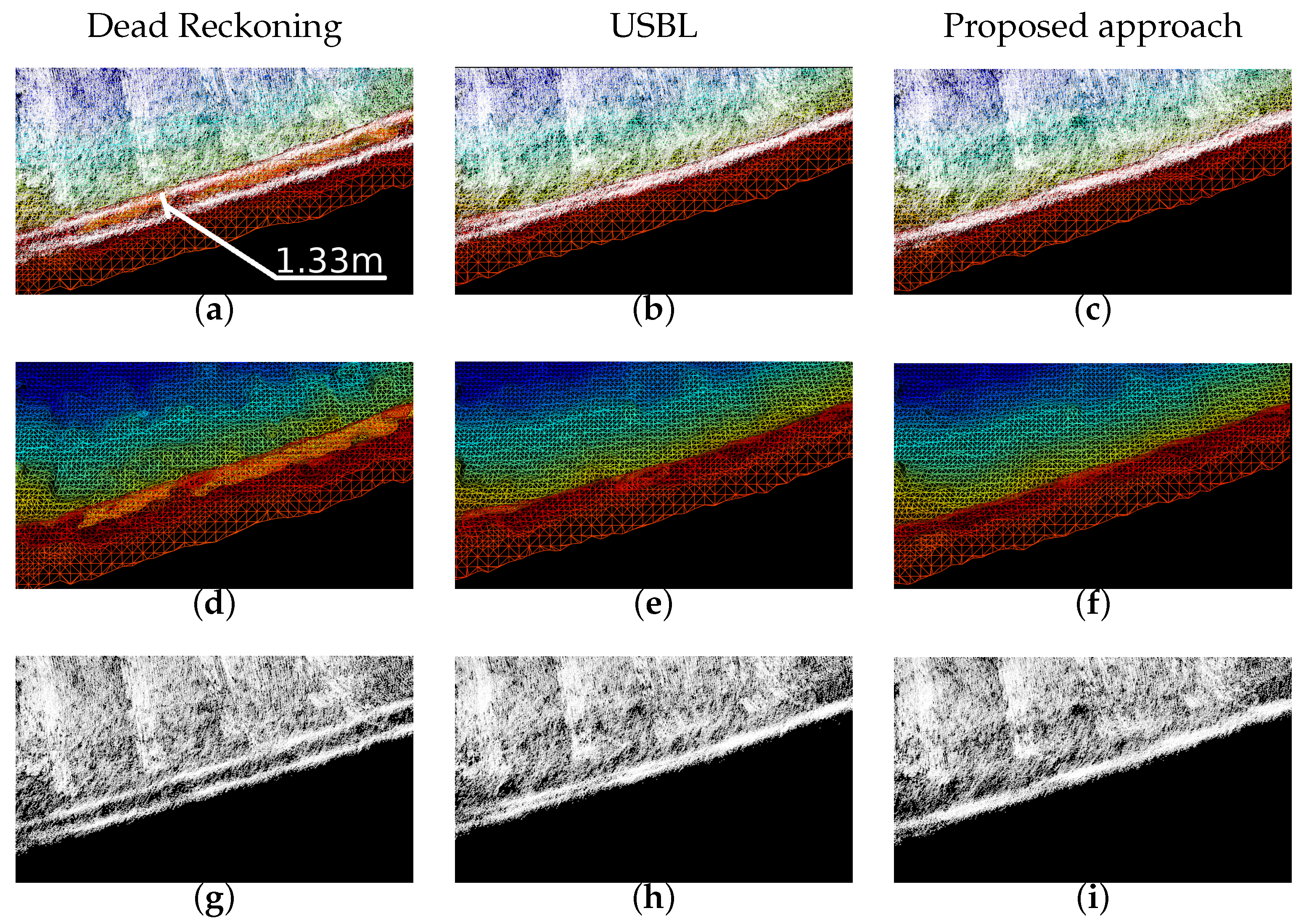
5.2. 3D Experiments
6. Conclusions
Acknowledgments
Author Contributions
Conflicts of Interest
References
- Panish, R.; Taylor, M. Achieving high navigation accuracy using inertial navigation systems in autonomous underwater vehicles. In Proceedings of the MTS/IEEE Oceans, Santander, Spain, 6–9 June 2011; pp. 1–7.
- Kinsey, J.C.; Whitcomb, L.L. Preliminary field experience with the DVLNAV integrated navigation system for oceanographic submersibles. Control Eng. Pract. 2004, 12, 1541–1549. [Google Scholar] [CrossRef]
- Batista, P.; Silvestre, C.; Oliveira, P. Single Beacon Navigation: Observability Analysis and Filter Design. In Proceedings of the American Control Conference (ACC), Baltimore, MD, USA, 30 June–2 Juny 2010; pp. 6191–6196.
- Vallicrosa, G.; Ridao, P.; Ribas, D. AUV Single Beacon Range-Only SLAM with a SOG Filter. IFAC Workshop Navig. Guid. Control Underw. Veh. 2015, 48, 26–31. [Google Scholar] [CrossRef]
- Thomas, H.G. GIB Buoys: An Interface Between Space and Depths of the Oceans. In Proceedings of the Workshop on Autonomous Underwater Vehicles, Cambridge, MA, USA, 20–21 August 1998; pp. 181–184.
- Mandt, M.; Gade, K.; Jalving, B. Integrateing DGPS-USBL position measurements with inertial navigation in the HUGIN 3000 AUV. In Proceedings of the 8th Saint Petersburg International Conference on Integrated Navigation Systems, Saint Petersburg, Russia, 28–30 May 2001.
- Carreño, S.; Wilson, P.; Ridao, P.; Petillot, Y.; Carreno, S.; Wilson, P.; Ridao, P.; Petillot, Y. A survey on Terrain Based Navigation for AUVs. In Proceedings of the MTS/IEEE Oceans, Seattle, WA, USA, 20–23 September 2010; pp. 1–7.
- Bailey, T.; Durrant-Whyte, H. Simultaneous Localization and Mapping (SLAM): Part II. IEEE Robot. Autom. Mag. 2006, 13, 108–117. [Google Scholar] [CrossRef]
- Eustice, R.; Pizarro, O.; Singh, H. Visually Augmented Navigation in an Unstructured Environment Using a Delayed State History. In Proceedings of the IEEE International Conference on Robotics and Automation (ICRA), New Orleans, LA, USA, 26 April–1 May 2004; Volume 1, pp. 25–32.
- Williams, S.; Mahon, I. Simultaneous Localisation and Mapping on the Great Barrier Reef. In Proceedings of the IEEE International Conference on Robotics and Automation (ICRA), New Orleans, LA, USA, 26 April–1 May 2004; Volume 2, pp. 1771–1776.
- Eustice, R.; Singh, H.; Leonard, J.; Walter, M.; Ballard, R. Visually Navigating the RMS Titanic with SLAM Information Filters. In Proceedings of the Robotics Science and Systems, Cambridge, MA, USA, 8–11 June 2005.
- Johnson-Roberson, M.; Pizarro, O.; Williams, S.B.; Mahon, I. Generation and Visualization of Large-Scale Three-Dimensional Reconstructions from Underwater Robotic Surveys. J. Field Robot. 2010, 27, 21–51. [Google Scholar] [CrossRef]
- Aykin, M.D.; Negahdaripour, S. On Feature Matching and Image Registration for Two-dimensional Forward-scan Sonar Imaging. J. Field Robot. 2013, 30, 602–623. [Google Scholar] [CrossRef]
- Hurtós, N.; Ribas, D.; Cufí, X.; Petillot, Y.; Salvi, J. Fourier-based Registration for Robust Forward-looking Sonar Mosaicing in Low-visibility Underwater Environments. J. Field Robot. 2015, 32, 123–151. [Google Scholar] [CrossRef]
- Leonard, J.J.; Carpenter, R.N.; Feder, H.J.S. Stochastic Mapping Using Forward Look Sonar. Robotica 2001, 19, 467–480. [Google Scholar] [CrossRef]
- Carpenter, R.N. Concurrent Mapping and Localization with FLS. In Proceedings of the Workshop on Autonomous Underwater Vehicles, Cambridge, MA, USA, 20–21 August 1998; pp. 133–148.
- Williams, S.; Newman, P.; Rosenbaltt, J.; Dissanayake, G.; Durrant-whyte, H. Autonomous underwater navigation and control. Robotica 2001, 19, 481–496. [Google Scholar] [CrossRef]
- Newman, P.; Leonard, J. Pure Range-Only Sub-Sea SLAM. In Proceedings of the IEEE International Conference on Robotics and Automation (ICRA), Taipei, Taiwan, 14–19 September 2003; pp. 1921–1926.
- Ribas, D.; Ridao, P.; Domingo, J.D.; Neira, J. Underwater SLAM in Man-Made Structured Environments. J. Field Robot. 2008, 25, 898–921. [Google Scholar] [CrossRef]
- Fairfield, N.; Jonak, D.; Kantor, G.A.; Wettergreen, D. Field Results of the Control, Navigation, and Mapping Systems of a Hovering AUV. In Proceedings of the 15th International Symposium on Unmanned Untethered Submersible Technology, Durham, NH, USA, 19–20 August 2007.
- Roman, C.; Singh, H. A Self-Consistent Bathymetric Mapping Algorithm. J. Field Robot. 2007, 24, 23–50. [Google Scholar] [CrossRef]
- Barkby, S.; Williams, S.B.; Pizarro, O.; Jakuba, M. A Featureless Approach to Efficient Bathymetric SLAM Using Distributed Particle Mapping. J. Field Robot. 2011, 28, 19–39. [Google Scholar] [CrossRef]
- Eliazar, A.; Parr, R. DP-SLAM: Fast, Robust Simultaneous Localization and Mapping without Predetermined Landmarks. In Proceedings of the IEEE International Conference on Robotics and Automation (ICRA), Taipei, Taiwan, 14–19 September 2003; Volume 18, pp. 1135–1142.
- Zandara, S.; Ridao, P.; Ribas, D.; Mallios, A.; Palomer, A. Probabilistic Surface Matching for Bathymetry Based SLAM. In Proceedings of the IEEE International Conference on Robotics and Automation (ICRA), Karlsruhe, Germany, 6–10 May 2013.
- Hernández, E.; Ridao, P.; Ribas, D.; Mallios, A. Probabilistic sonar scan matching for an AUV. In Proceedings of the IEEE/RSJ International Conference on Intelligent Robots and Systems (IROS), St. Louis, MO, USA, 10–15 October 2009; pp. 255–260.
- Mallios, A.; Ridao, P.; Ribas, D.; Maurelli, F.; Petillot, Y. EKF-SLAM for AUV navigation under probabilistic sonar scan-matching. In Proceedings of the IEEE/RSJ International Conference on Intelligent Robots and Systems (IROS), Taipei, Taiwan, 18–22 October 2010; pp. 4404–4411.
- Burguera, A.; Oliver, G.; González, Y. Scan-Based SLAM with Trajectory Correction in Underwater Environments. In Proceedings of the IEEE/RSJ International Conference on Intelligent Robots and Systems (IROS), Taipei, Taiwan, 18–22 October 2010; pp. 2546–2551.
- Mallios, A.; Ridao, P.; Ribas, D.; Hernández, E. Scan Matching SLAM in Underwater Environments. Auton. Robots 2014, 36, 181–198. [Google Scholar] [CrossRef]
- Burguera, A.; González, Y.; Oliver, G. A Probabilistic Framework for Sonar Scan Matching Localization. Adv. Robot. 2008, 22, 1223–1241. [Google Scholar] [CrossRef]
- Smith, R.; Self, M.; Cheeseman, P. Chapter 3: Estimating Uncertain Spatial Relationships in Robotics. In Autonomous Robot Vehicles; Cox, I.J., Wilfong, G.T., Eds.; Springer: New York, NY, USA, 1990; Volume 1, pp. 167–193. [Google Scholar]
- Kanazawa, Y.; Kanatani, K. Reliability of fitting a plane to range data. IEICE Trans. Inf. Syst. 1995, E78D, 1630–1635. [Google Scholar]
- Weingarten, J. Feature-based 3D SLAM. Ph.D. Thesis, École Polytechinque Fédérale de Lausanne, Lausanne, Switzerland, 6 September 2006. [Google Scholar]
- Pathak, K.; Vaskevicius, N.; Birk, A. Revisiting uncertainty analysis for optimum planes extracted from 3D range sensor point-clouds. In Proceedings of the IEEE International Conference on Robotics and Automation (ICRA), Kobe, Japan, 12–17 May 2009; pp. 1631–1636.
- Palomer, A.; Ridao, P.; Ribas, D.; Mallios, A.; Vallicrosa, G. Octree-Based Subsampling Criteria for Bathymetric SLAM. In Proceedings of the XXXV Jornadas de Automática, Valencia, Spain, 3–5 September 2014; pp. 1–6.
- Williams, S.; Pizarro, O.; Mahon, I.; Johnson-roberson, M. Chapter 9: Simultaneous Localisation and Mapping and Dense Stereoscopic Seafloor Reconstruction Using an AUV. In Experimental Robotics: The Eleventh International Symposium; Springer: Berlin, Geramny, 2009; pp. 407–416. [Google Scholar]
- Ribas, D.; Palomeras, N.; Ridao, P.; Carreras, M.; Mallios, A. Girona 500 AUV: From Survey to Intervention. IEEE ASME Trans. Mechatron. 2012, 17, 46–53. [Google Scholar] [CrossRef]
- Roman, C.; Singh, H. Consistency based error evaluation for deep sea bathymetric mapping with robotic vehicles. In Proceedings of the IEEE International Conference on Robotics and Automation (ICRA), Orlando, FL, USA, 15–19 May 2006; pp. 3568–3574.
- Kazhdan, M.; Hoppe, H. Screened Poisson Surface Reconstruction. ACM Trans. Graph. 2013, 32, 1–13. [Google Scholar] [CrossRef]


| Experiment | ||
|---|---|---|
| 2.5D | 3D | |
| Minimum patch size (Section 2.2) | 30 m | - |
| Maximum patch size (Section 2.2) | 80 m | - |
| Normal occupancy (Section 2.2) | 23% | - |
| Patch overlapping (Section 4.2) | 30% | 30% |
| Point cloud subsampling (Section 3.4) | 0.5 m | 1.5 m |
| Relative displacement to switch from point-to-point to point-to-plane association (Section 3) | 1 cm | 1 cm |
| Sum | Mean | #Cells | |
|---|---|---|---|
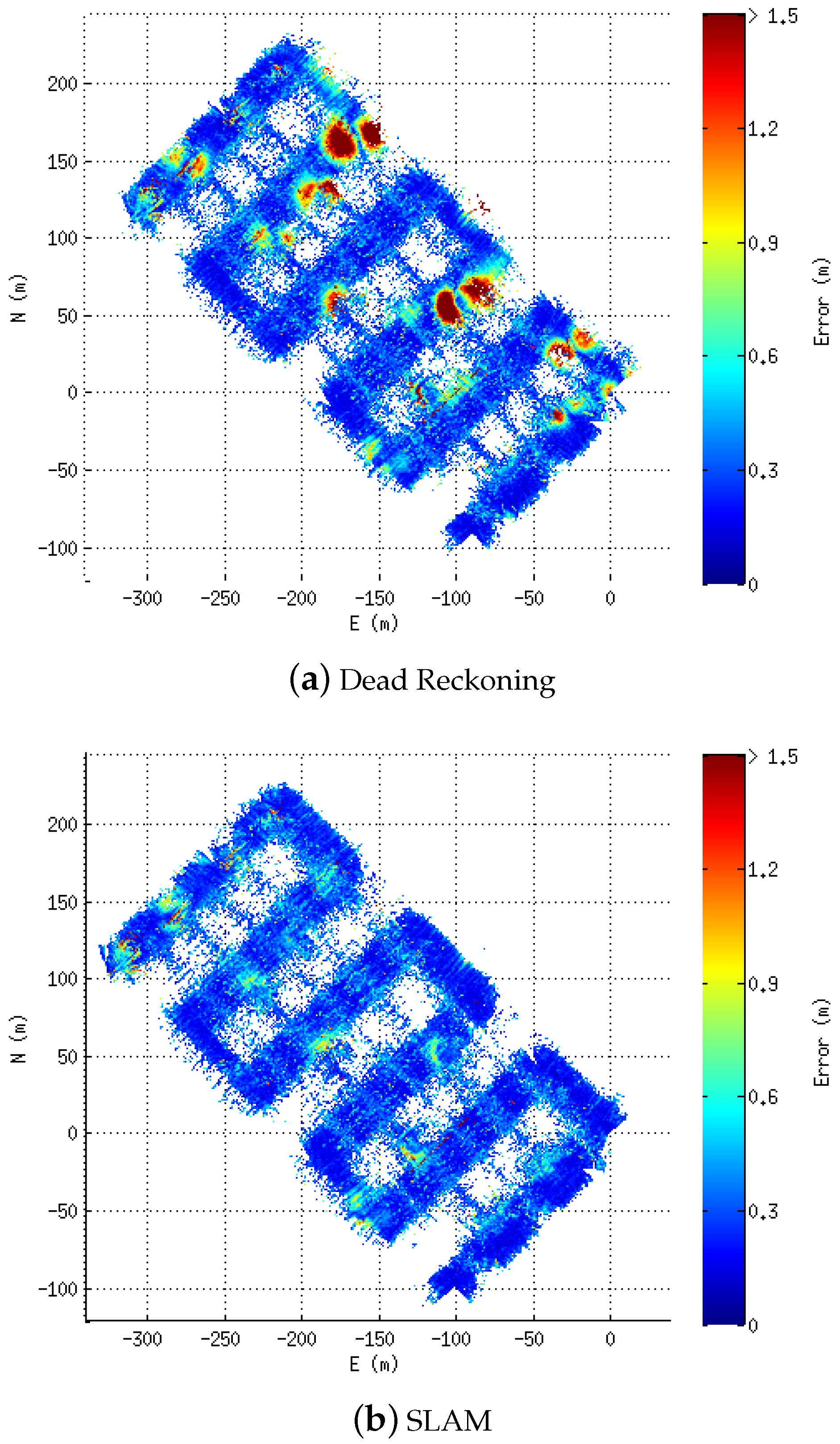
| Dead reckoning | 70,986.2 | 0.3988 | 37,3121 |
| SLAM | 57,521.8 | 0.3223 | 36,5014 |
| Improvement * | 18.97% | 19.2% | 2.17% |
© 2016 by the authors; licensee MDPI, Basel, Switzerland. This article is an open access article distributed under the terms and conditions of the Creative Commons Attribution (CC-BY) license (http://creativecommons.org/licenses/by/4.0/).
Share and Cite
Palomer, A.; Ridao, P.; Ribas, D. Multibeam 3D Underwater SLAM with Probabilistic Registration. Sensors 2016, 16, 560. https://doi.org/10.3390/s16040560
Palomer A, Ridao P, Ribas D. Multibeam 3D Underwater SLAM with Probabilistic Registration. Sensors. 2016; 16(4):560. https://doi.org/10.3390/s16040560
Chicago/Turabian StylePalomer, Albert, Pere Ridao, and David Ribas. 2016. "Multibeam 3D Underwater SLAM with Probabilistic Registration" Sensors 16, no. 4: 560. https://doi.org/10.3390/s16040560
APA StylePalomer, A., Ridao, P., & Ribas, D. (2016). Multibeam 3D Underwater SLAM with Probabilistic Registration. Sensors, 16(4), 560. https://doi.org/10.3390/s16040560