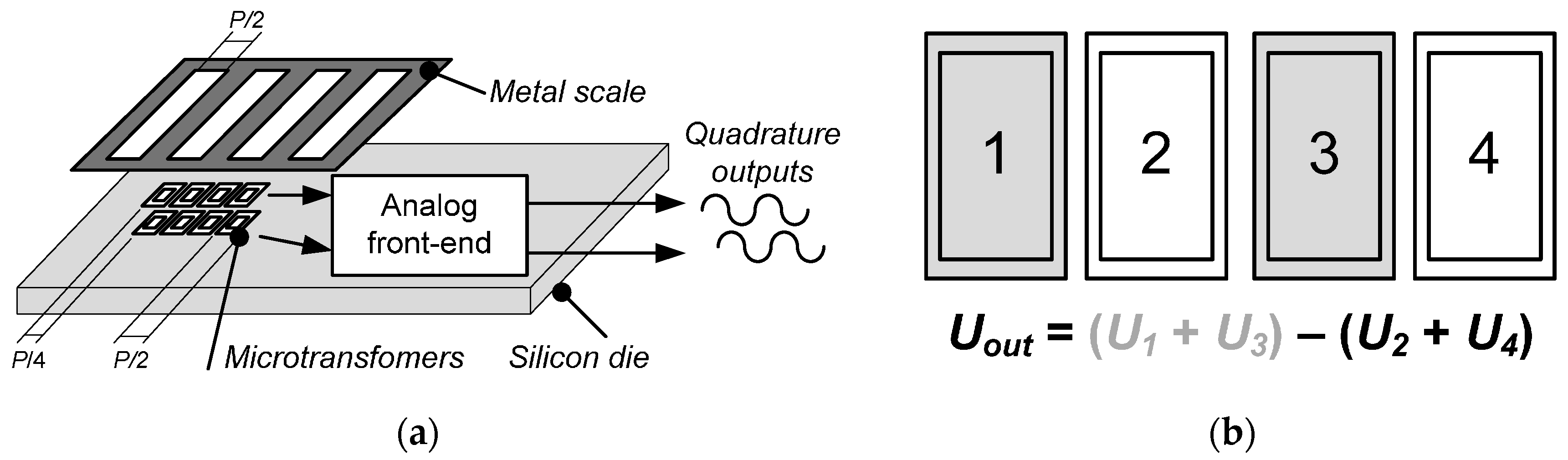
The design of the prototype microsystem with a piece of a target scale is presented in
Figure 2a. It consists of a silicon die comprising the microtransformers along with analog front-end electronics for signal conditioning and processing. The external dimensions of the primary and the secondary microcoil of the microtransformer are 750 by 495 µm and 576 by 321 µm, respectively, with the scale period
P of 1 mm. The center-to-center distance of two adjacent microtransformers equals
P/2,
i.e., 500 µm. As the microsystem is intended to find its final application in an incremental linear encoder, it is desired that its outputs have a round period, facilitating the interpolation and the evaluation of the signal. Furthermore, the period size and consecutively the microtransformer dimensions were also directed by the limited silicon area for prototyping the ASIC.
The number of microtransformers can be increased to improve the output signal level by summing the output voltages of coils with the same position inside a distinct scale period. The summation scheme for the discussed sensor system prototype comprising four microtransformers per channel is presented in
Figure 2b. As presented in
Figure 2a, the sensor is comprised of two channels shifted for a quarter of the scale period, thus yielding quadrature output signals.
2.1. Microtransformer Design and Its Model Circuit
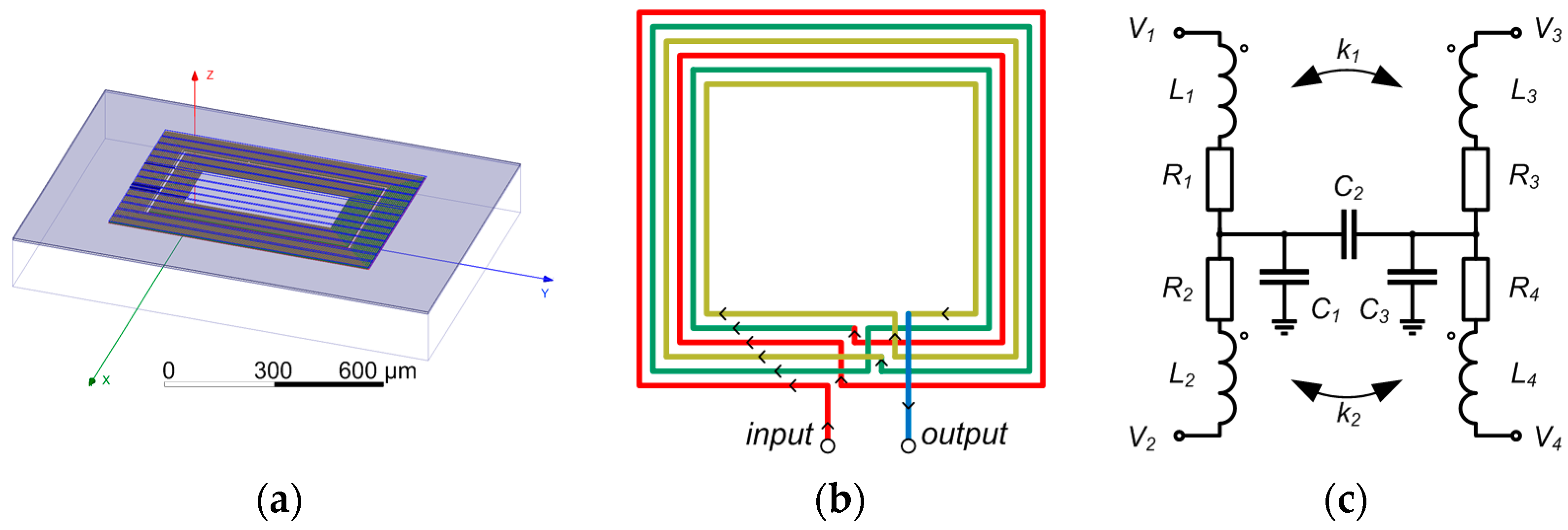
A 3D model of the microtransformer is presented in
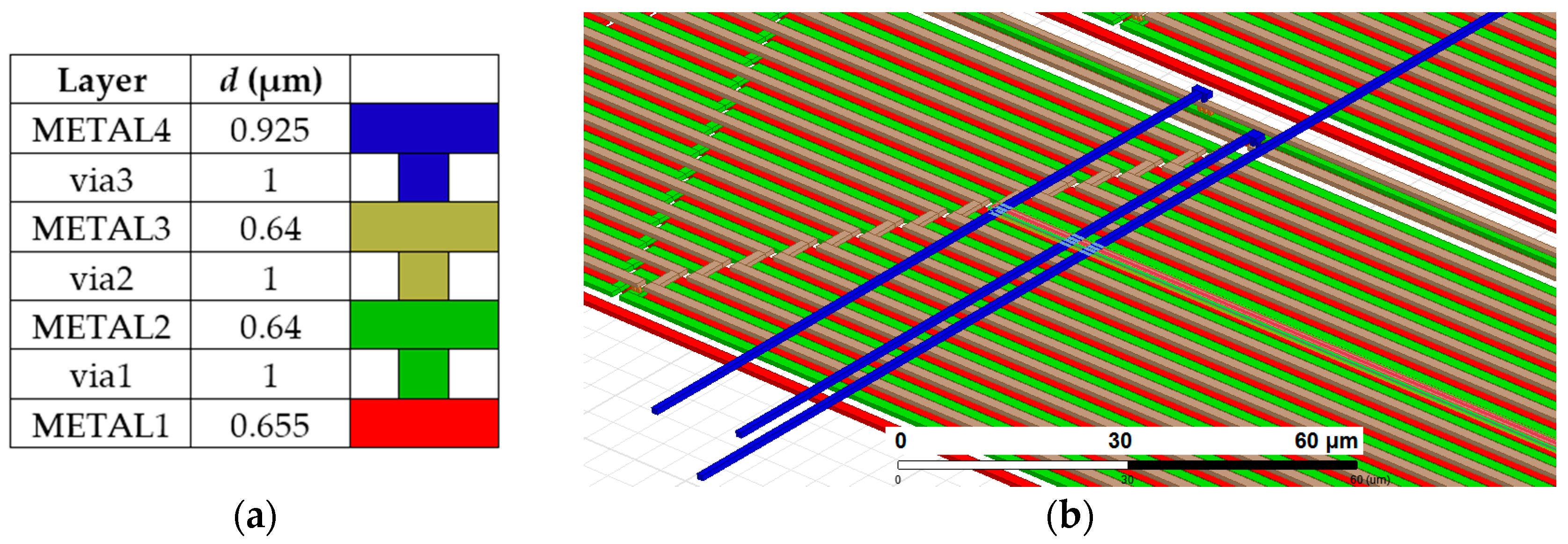
Figure 3a and
Figure 4b. Both the primary and the secondary winding comprise 45 windings in three metal layers (15 per layer) with the bridging interconnections realized in the fourth metal layer. A standard 350 nm microtechnologic process is used. The winding trace width is 1.5 µm and the spacing between the traces is 0.2 µm. The structure of the layered winding is presented in
Figure 3b. Only one winding (primary) is shown with two turns per layer to clearly illustrate the principle. The current flow direction is indicated with arrows. The secondary winding with the same structure is placed concentrically in the middle of the primary winding. The inter-winding capacitance is reduced by placing neighboring windings in different heights. This is believed to bring an approximate 60% reduction of the inter-winding capacitance (simulated using FEM as the ratio between the capacitance of two parallel rectangular conductors with trace dimensions, placed in the same and in another metal layer).The trace width was chosen according to process specification of recommended maximum current per metal trace width (1 mA/µm), to allow the nominal excitation current of 1 mA. The trace was widened to 1.5 µm as a safety measure to prevent the heating of the ASIC, which would affect the operation of the electronics. A rectangular coil shape was selected to maximize the silicon space utilization. The turn number was mainly directed by the target primary resistance range of 5 kΩ: the excitation voltage amplitude limit is limited to 5 V, which gives a nominal current of 1 mA at that resistance. This voltage limit is equal to the ASIC supply voltage and has to be followed due to the requirements of the IC ESD protection structures. The turn count also governs the windings’ inductance and their coupling factor
k, which is maximized by positioning the windings concentrically.
A model circuit of a single microtransformer (without the target) is presented in
Figure 3c. Connection Terminals 1 and 2 are used for the introduction of the primary (excitation) current into the system. The induced voltage is measured at Terminal 3 of the microtransformer. Terminal 4 is used for the reference potential connection,
i.e., the DC bias voltage for the amplifier.
ANSYS Electronic Desktop (Q3D Extractor) software package was used to determine the model circuit parameters. A GDS file, including the metal layers from the IC layout database, was imported into the software. The model circuit extraction process is not extensively time- and memory-consuming: it took approximately 45 min on 16 cores of a Xeon E5-2680 processor, requiring less than 2 GB of RAM. The extraction results are given in
Table 1.
The model circuit component values indicate high winding resistances (e.g., 5314 Ω for the primary). This is due to the small cross-sectional area of the trace and the large number of windings. The total primary load resistance of all eight microtransformers (wired in parallel in the IC) is therefore 664 Ω.
The capacitances are relatively large, causing a significant capacitive coupling between the primary and the secondary winding. However, this effect is effectively mitigated by the symmetry of the coils forming a pair and the differential operation of the sensor: since the capacitively transferred signal is equal for all microtransformers, it is effectively subtracted out of the differential signal. Also, the ASIC substrate ground must be well-defined to suppress the coupling between the windings through the substrate.
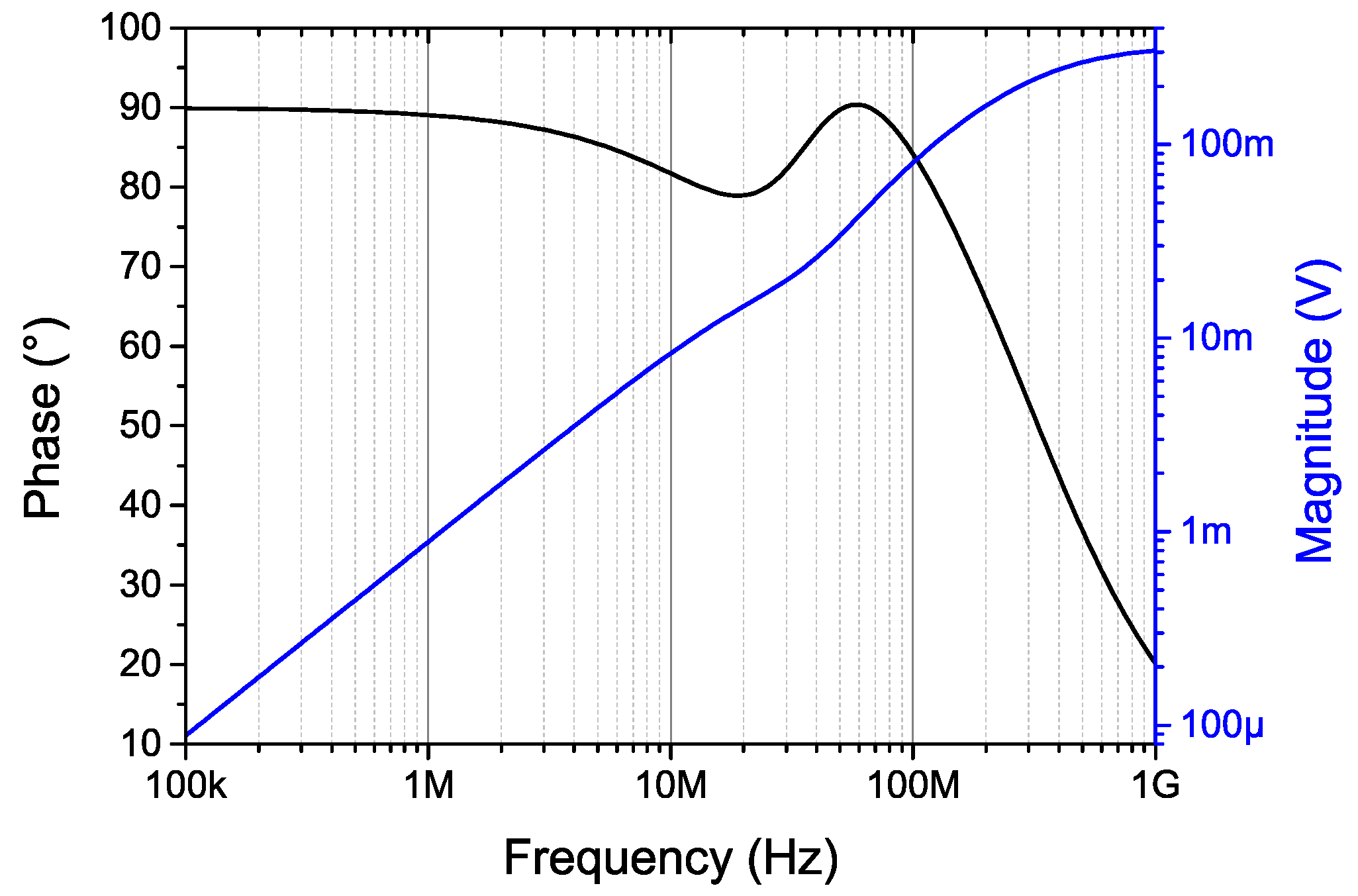
The simulated transfer function of the microtransformer is presented in
Figure 5. Its bandwidth (over 100 MHz) does not limit the system operation, which is instead limited by the analog front-end electronics to approximately 10 MHz.
High winding resistances result in strongly damped resonant circuits formed by the microtransformers’ inductances and parasitic capacitances. The approximate quality factor
Q of the primary winding is 0.30 with a resonant frequency of 111 MHz. For the secondary winding, the quality is 0.42 and the resonant frequency is 183 MHz. These resonances are difficult to discern from
Figure 5 due to strong resistive damping.
The use of such in-chip high-resistance and high-inductance microcoils with thin conductor widths in the resonance is limited due to their low Q and high resonant frequency. Therefore, the presented microsystem relies on non-resonant inductive coupling. We found the microtransformer parameters satisfactory for the task.
However it would be interesting to investigate the CMOS-technology feasibility and performance of microtransformers using wider traces, similar to the displacement-sensing inductor reported in [
18] with a significantly larger size (2 by 2 mm), a quality factor of 14 and a lower resonance frequency (9.4 MHz).
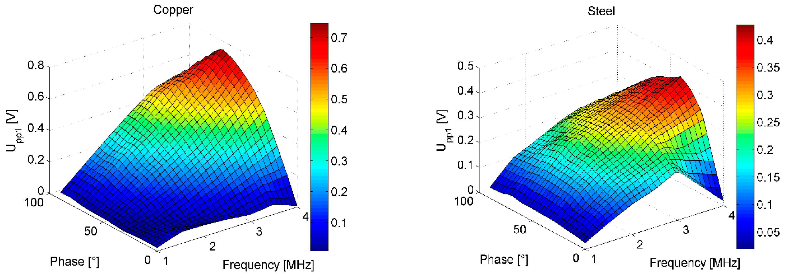
2.2. Simulations of the Target Effect
The microtransformer transfer function presented in
Figure 5, indicates an output magnitude range of approximately 1–10 mV in the frequency range of 1–10 MHz if 1 V excitation is used. However, a full 3-D simulation needs to be carried out to determine the modulation parameters of the output signal if a target scale is moved over the microtransformers. COMSOL Multiphysics FEM simulation software has been used for the task.
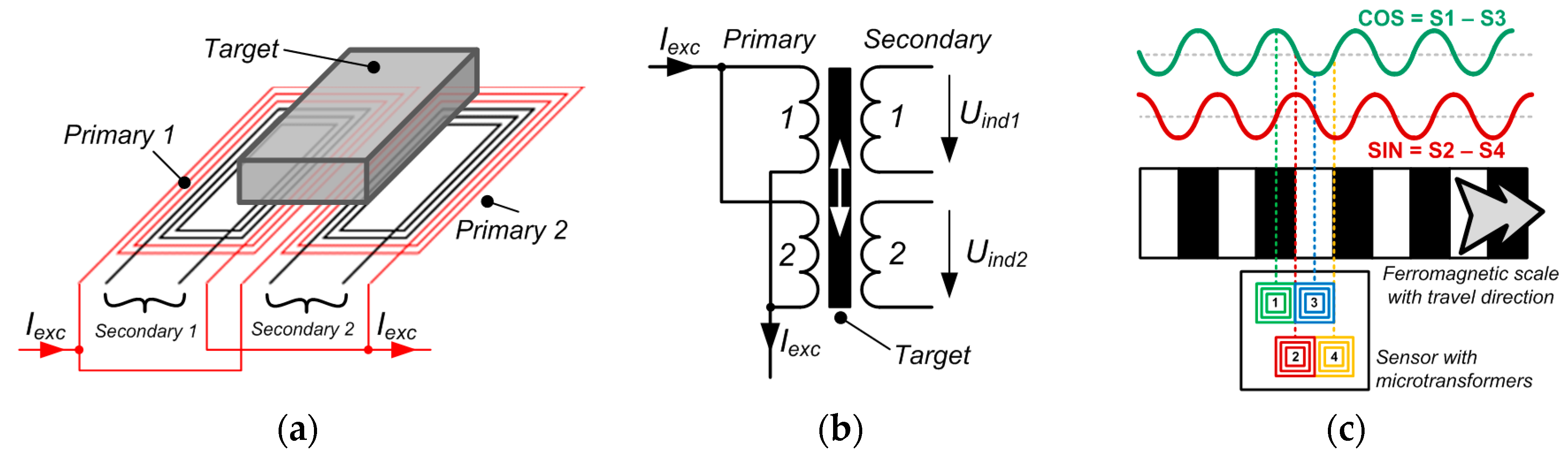
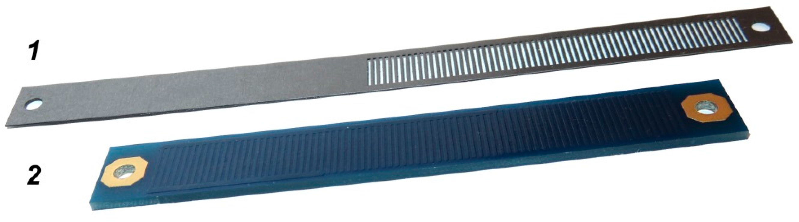
The performance of a microtransformer pair (as presented in
Figure 1a) has been evaluated for a copper scale fabricated as a printed circuit board (PCB), and a laser-cut ferromagnetic scale, made from transformer steel (Acroni M330-35A [
26]). The simulated target scales were designed to represent the actual scales used for the microsystem characterization, presented in
Figure 6.
In the simulator, the conductivity of copper was set to 5.9 × 10
7 S/m, while the conductivity of steel was set to 2.2 × 10
6 S/m according to [
27] (p. 14/3). The relative magnetic permeability of the steel was set to a generic value of 10 according to [
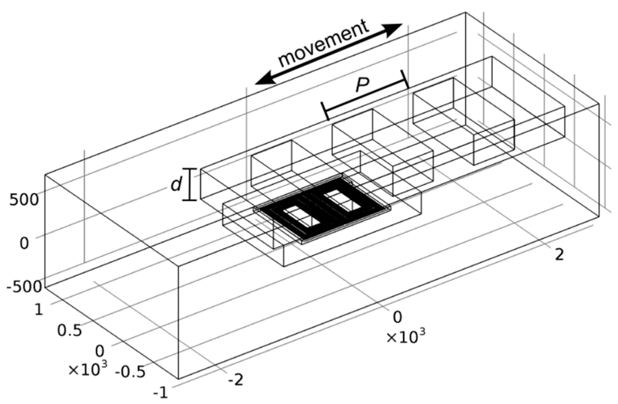
28], since we have been unable to obtain exact electromagnetic properties for the used scale material. The microtransformer was modeled as a planar rectangular spiral coil. A 3-D image of the simulated structure is presented in
Figure 7.
Since the cross-section of the microtransformer aluminum conductors (0.64 by 1.5 µm) is small in comparison to the dimensions of the target and to the skin depth of aluminum (37 µm at 5 MHz [
29], p. 315), which assures an uniform current distribution in the conductor cross-section), the conductors can be modeled as current-carrying lines, significantly reducing the complexity of the FEM mesh. Despite this simplification, a displacement sweep with the target position calculated in 30 steps of a 1 mm displacement range still takes several hours for a single frequency, requiring more than 30 GB of RAM in a workstation using 16 cores of an Intel Xeon E5-2680 processor. Due to the complexity of the simulation we have chosen to simulate only a single pair of microtransformers instead of two prototyped pairs.
The primary current amplitude was set to 1 mA, which approximately corresponds to the excitation voltage amplitude of 5 V at 5 kΩ primary winding resistance. The simulation was carried out in the complex domain. The vertical distance between the target and the microtransformers was 200 µm. The secondary induced voltage can be determined using line integration of the vector magnetic potential
A over a closed loop
L of the secondary winding ([
29], p. 192 and 197):
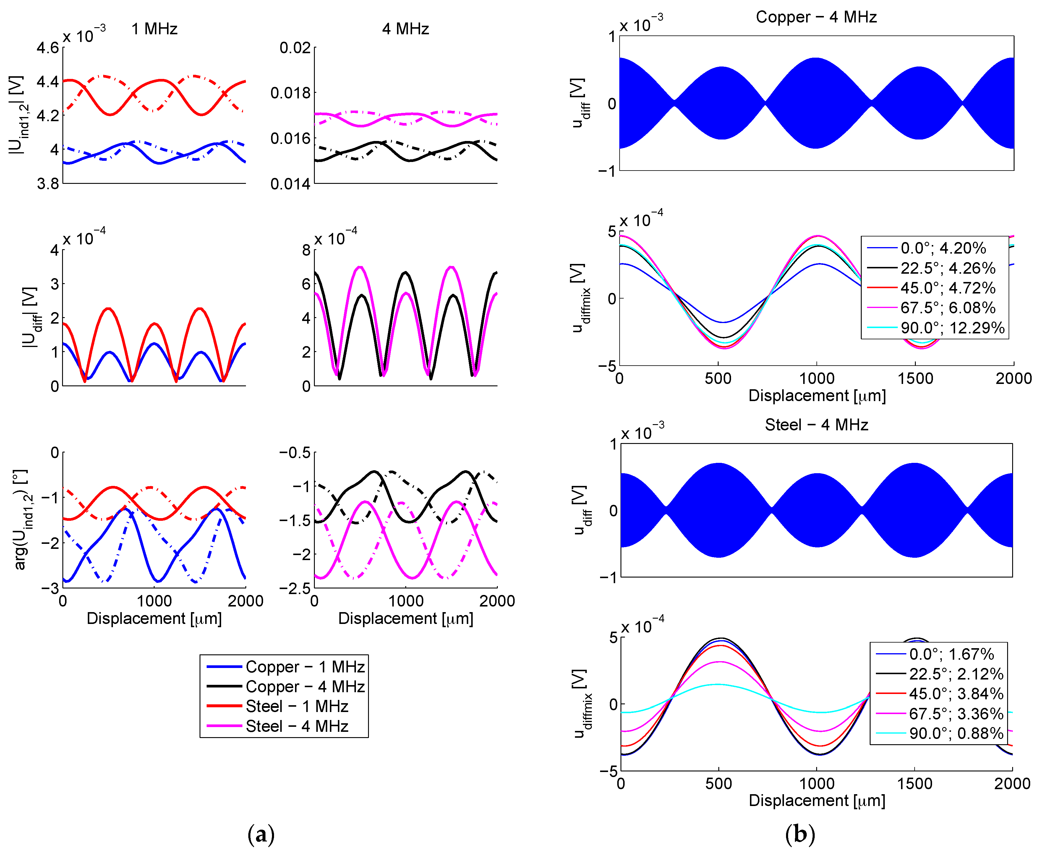
For each microtransformer, an array of complex induced voltages is returned, corresponding to the swept scale positions. Amplitudes and phase angles of the two microtransformer output signals (
Uind1,
Uind2) for two target materials and two operating frequencies (1 and 4 MHz) are presented in
Figure 8a.
The amplitude of the differential signal (
Udiff =
Uind1 −
Uind2) are also shown. Note that the simulated signals’ phases do not exhibit a 90° inductive shift, since the secondary signals originate in line current, which does not have an inductive character. The described inverse operation for the ferromagnetic and the conductive target scale is clearly visible in
Figure 8a: magnitudes of displacement-dependent induced voltages |
Uind1,2| for the copper scale are always lower due to an increased eddy-current induced energy caused by larger copper conductivity. Furthermore, the maxima and the minima of voltages |
Uind1,2| oppose each other for the two materials. At 1 MHz excitation frequency, the ferromagnetic effect manifested in steel overcomes the eddy-current effect in copper, resulting in greater modulation (larger |
Udiff|). At 4 MHz, the modulation approximately equalizes, indicating the increasing prominence of the eddy-current effects with rising frequency. As the phase modulation (arg (
Uind1,2)) is related to the eddy current losses, its characteristics are not opposite for the two materials. It can be seen how the shape of the differential signal (converted to the time domain in
Figure 8b) is much more sinusoidal in comparison to the direct transformer outputs’ amplitudes |
Uind1,2|, indicating the importance of the differential operation of such sensors.
The secondary voltages are then subtracted and transformed from the complex domain into a time-domain signal
udiff, shown in
Figure 8b. The actual simulated results ranging between 0–1000 µm are duplicated, resulting in 0–2000 µm range, to better illustrate the signals’ shape. For the purpose of the analysis of the demodulation principle, an arbitrary frequency
fc of this signal can be chosen, in this case 1000-times higher than the frequency of the scale movement. During the operation of an actual device, this ratio can be much higher; however the usage of a lower ratio does not affect the illustration of the principle.
2.2.1. Signal Demodulation
The synchronous demodulation method (also: coherent detection) is based on mixing (
i.e., multiplying) the modulated signal with a sinusoidal signal of the same carrier frequency
fc and phase ϕ
mix. The resulting signal is composed of an AC signal with 2
fc frequency and a DC component in a linear correlation with the modulation of the signal and the mixing signal phase ϕ
mix [
30] (p. 96).
To suppress the AC component of the signal
Udiff, a low-pass filter (LPF) is employed. A fourth-order Butterworth LPF with the 3dB frequency margin of 1%
fc was used, resulting in the demodulated signal
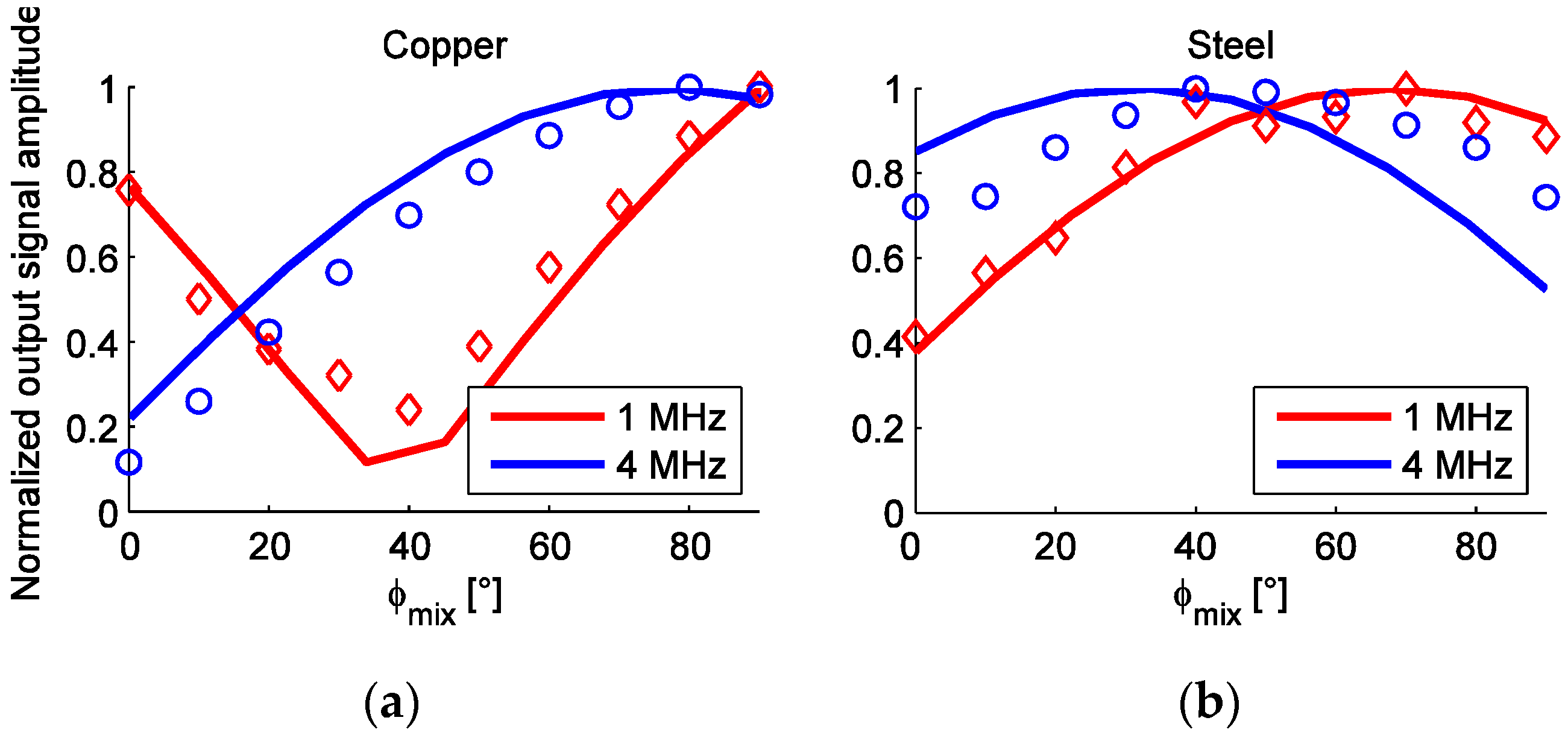
udiffmix. The shape of this signal depends on different material and geometric properties of each scale. The result of the coherent demodulation is also strongly dependent on ϕ
mix, as demonstrated in
Figure 8b. Therefore, an optimal mixing signal phase ϕ
mix can be determined for each target configuration to maximize the output signal amplitude, as will be demonstrated in
Section 3 when discussing the microsystem characterization.
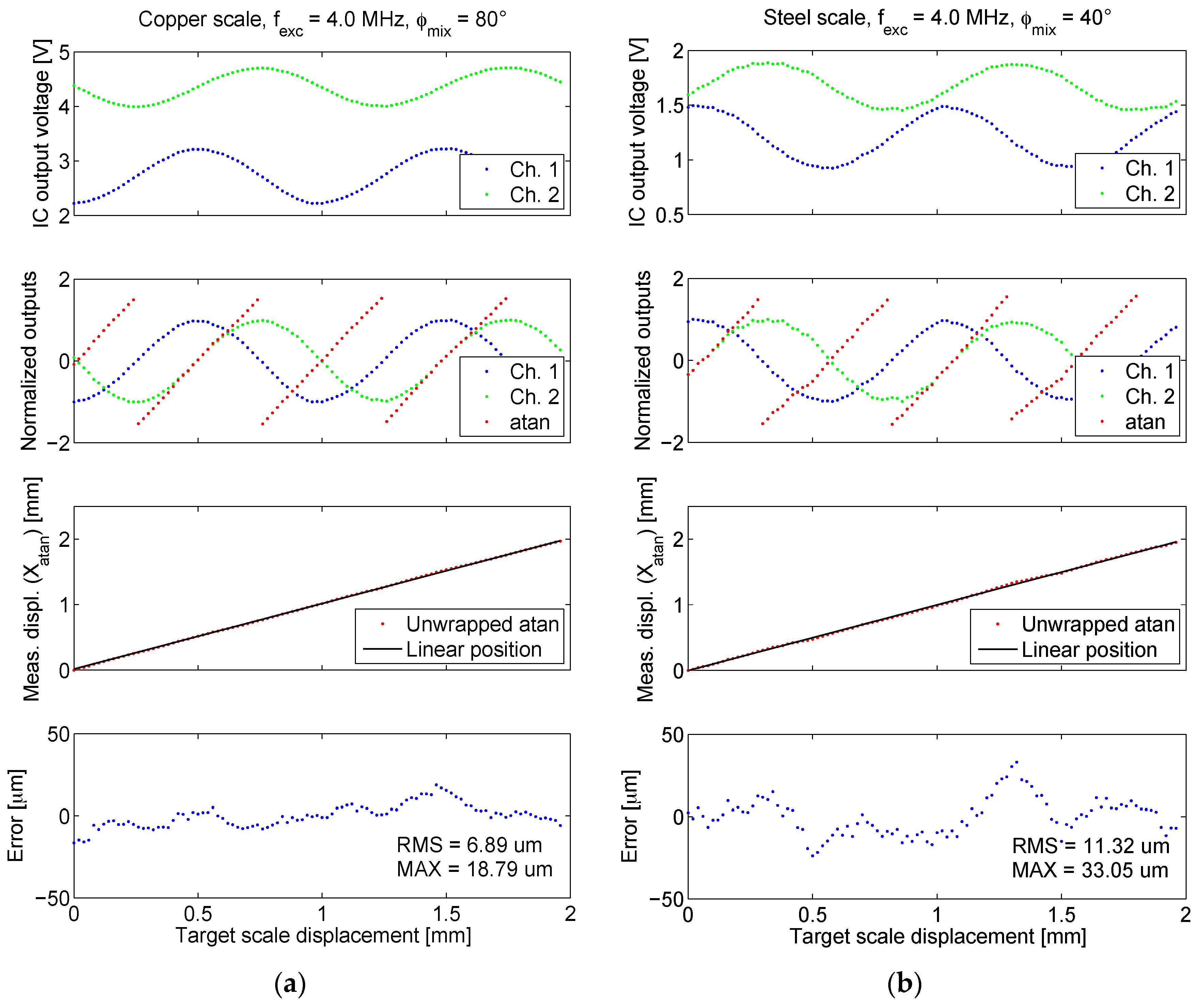
To establish the linear position using the arctangent of quadrature signals (Equation (1)), a sinusoidal shape of the position-dependent output signal is required. As its figure of merit, the total harmonic distortion (THD) [
31] (p. 83) for the first five harmonics of the demodulated signal has been calculated, which is also stated next to the corresponding phases ϕ
mix in
Figure 8b.
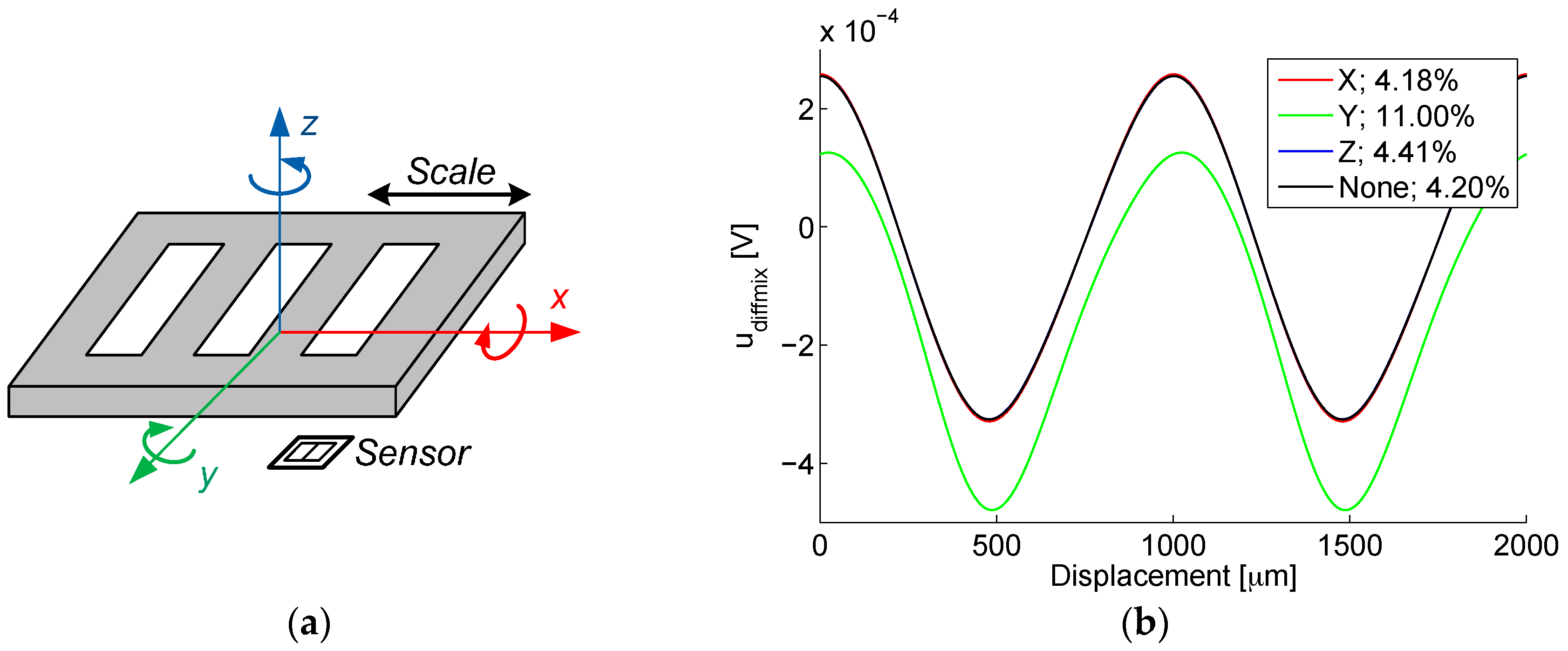
2.2.2. Scale Tilting
Another issue worth addressing is the tilting of the scale over the sensor, which is inevitable at a sensor operating in an actual application. The tilting was analyzed using the same methodology and the same simulation setup as presented in
Section 2.2. The target scale was rotated for an angle of 3° in three dimensions, as depicted in
Figure 9a. The simulation was carried out with a copper scale at 4 MHz and ϕ
mix = 0°; its results are shown in
Figure 9b.
The simulation results show that the rotation of the target scale in x and z axis does not significantly affect the output differential signal udiffmix, as the results virtually align with the situation without tilting (None). However, a notable deviation occurs when the target is tilted longitudinally (y axis): each microtransformer in the pair has a different target coupling characteristics due to the different height of the scale over each microtransformer.
Their outputs are not complementary any more, resulting in increased offset and distortion of the differential signal, which is also reflected in the THD increase. For other two (x and z) axes, the effect of the tilt is almost equal for both microtransformers in a pair, so it is still compensated by the subtraction of their output signals.
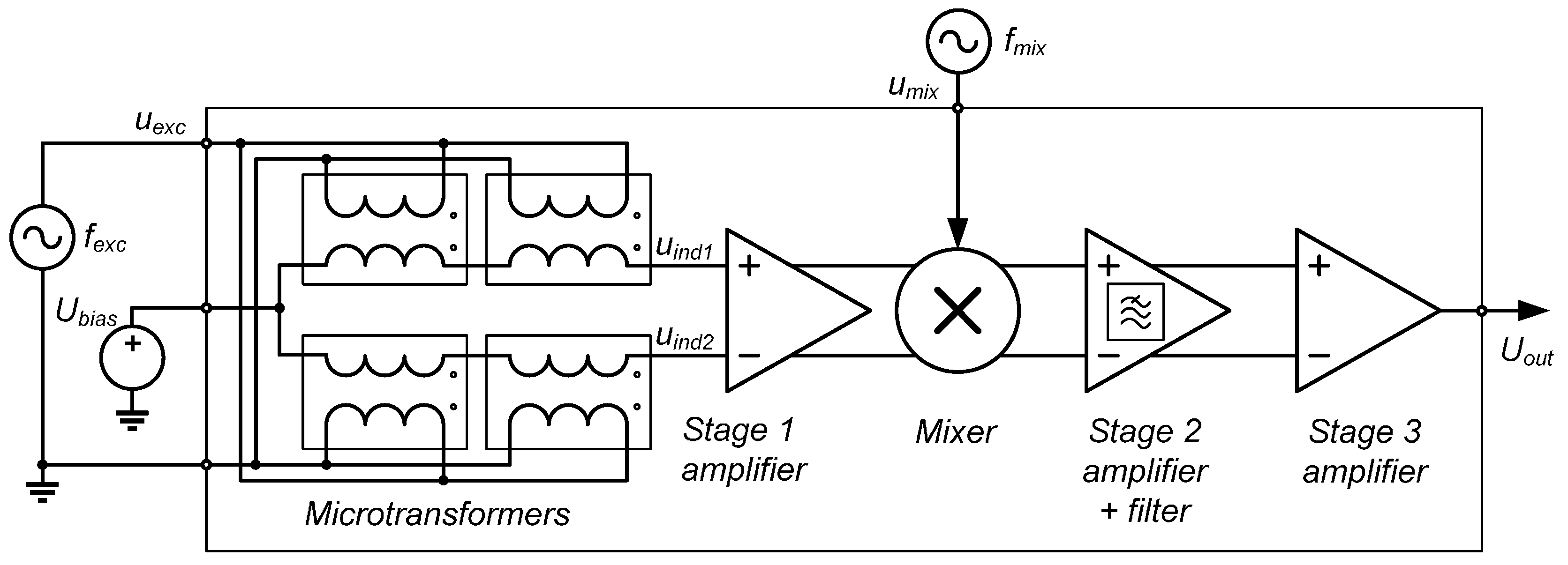
2.3. ASIC Design and Simulation
We have already introduced the synchronous demodulation method for the differential microtransformer signal. This section describes the actual measurement channel realized in the prototype ASIC, depicted schematically in
Figure 10. Cadence Virtuoso Analog Design Environment software (Spectre Simulator) was used as the main tool in the analog front-end design process.
As previously explained, two differential transformers are wired serially to increase the signal level. Fully differential design is used for signal amplification, mixing, and filtering, due to the symmetric nature of the problem (subtracting the signals of two identical microtransformers), improved noise immunity and common mode rejection as well as simpler DC biasing ([
32], p. 100–102). The amplification is realized in three stages. Due to different requirements of each particular stage, three different operational amplifiers had to be designed. The first wideband amplifier in the chain employs a telescopic topology due to its required high frequency range ([
32], p. 297–299), featuring a simulated DC closed-loop gain of 6 and a gain-bandwidth product of 72 MHz with two serially connected microtransformers at the input. The level of the output signal can be controlled by the amplitude of the mixing signal. A single-balanced Gilbert cell mixer is used ([
33], p. 418). The second-stage DC gain is 15. This amplifier employs a simpler Miller topology ([
32], p. 296).
The second-stage amplifier also functions as a LPF for the suppression of the excitation frequency
fexc: its 3dB corner frequency is designed to be 325 kHz. This relatively high corner frequency allows for an optional operation of the system with heterodyne mixing ([
30], p. 128), if the frequency
fmix is set to a value different from
fexc, resulting in a mixer output signal with a frequency of
fout = |
fexc −
fmix| (another component with a frequency of
fexc +
fmix is suppressed by the LPF). The third-stage amplifier subtracts the signals of the positive and negative signal path, amplifies this difference with a gain of 100, and serves as the output buffer.
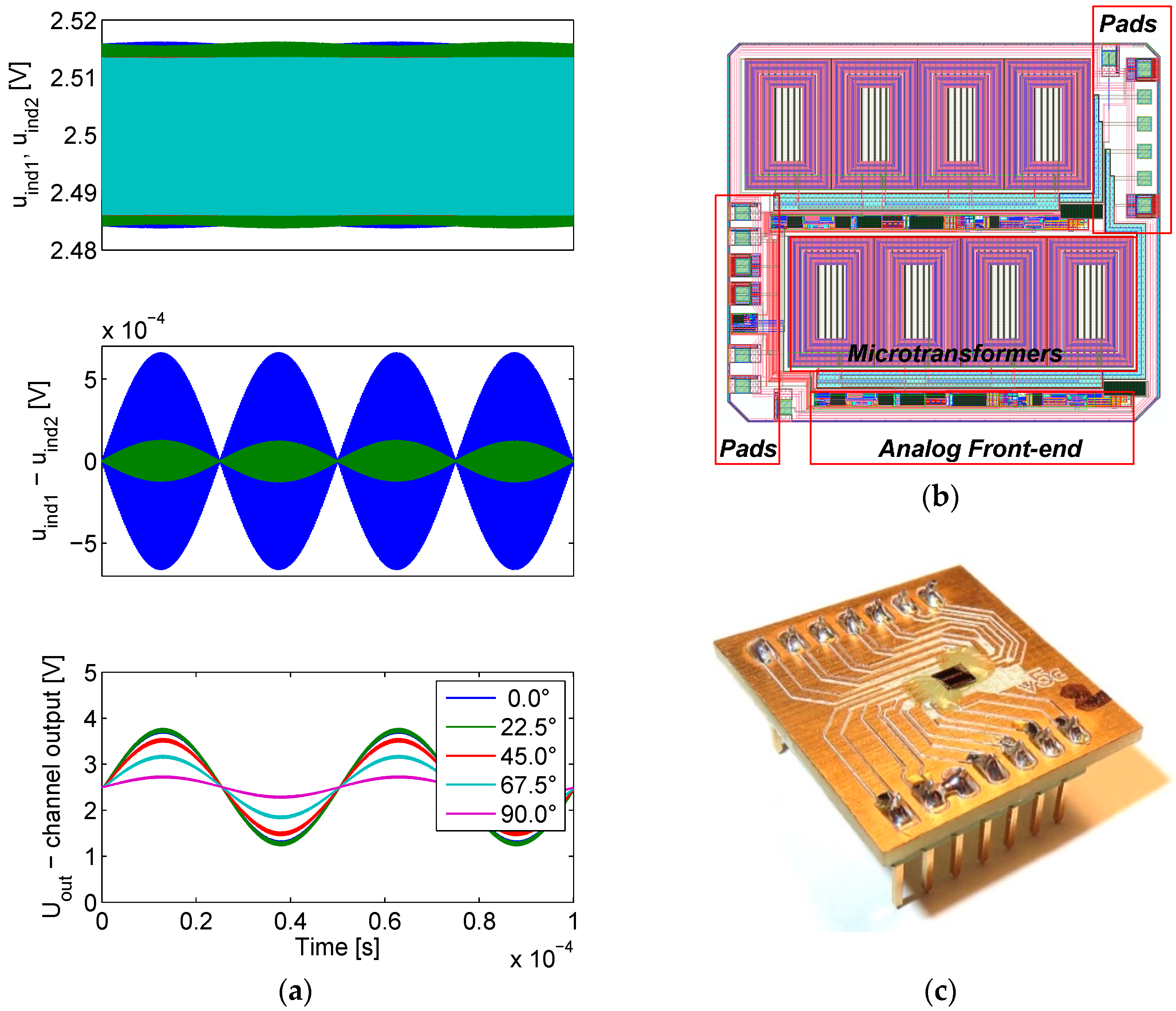
The results of the IC simulation are presented in
Figure 11a. The circuit presented in
Section 2.1 has been used to model the differential transformers. The scale modulation (with a frequency
fscale) was introduced into the model by sinusoidally varying the value of inductor coupling coefficient
k, resulting in a symmetric amplitude-only modulation. For this purpose, the model circuit was rewritten into a high-level analog behavioral model description language Verilog-A [
34], which allows for the dynamic variation of the model parameters. The modulation was configured to approximate the performance of the FEM-simulated copper scale at 4 MHz when the secondary windings had no load connected. An agreement has been found when the coupling coefficient function was set to:
When the amplifier is connected to the microtransformer, the coil output signals are reduced due to the impedance of the amplifier feedback connected to their output. The effect of this loading is visible in the middle chart in
Figure 11a, showing the unloaded differential signal in blue color, and the loaded differential signal in green. The top chart also shows the unloaded (green and blue) and loaded (light green and red) positive and negative coil output signals.
Since the microtransformer and the first-stage amplifier introduce respective 90° and 180° (low-frequency values) phase shifts, with the actual simulated total phase shift being 243° at 4 MHz due to poles in the transfer characteristic, this value is added to the simulated mixing signal phase ϕmix, assuring the mixing and demodulated signal coherency at ϕmix = 0°.
The excitation voltage
uexc and mixing voltage
umix amplitudes are set to the same values used later in the characterization of the IC,
i.e., 2.5 V and 0.25 V respectively. The bottom graph in
Figure 11a indicates that the amplitude maximum of the output signal
Uout occurs when ϕ
mix = 0°. Since the phase modulation is not modeled, the mixing signal and the signal being demodulated are in-phase at zero ϕ
mix, resulting in maximal amplitude. Such simulations that neglect the phase modulation of the target have been used primarily to adjust the gain of the amplifier chain.
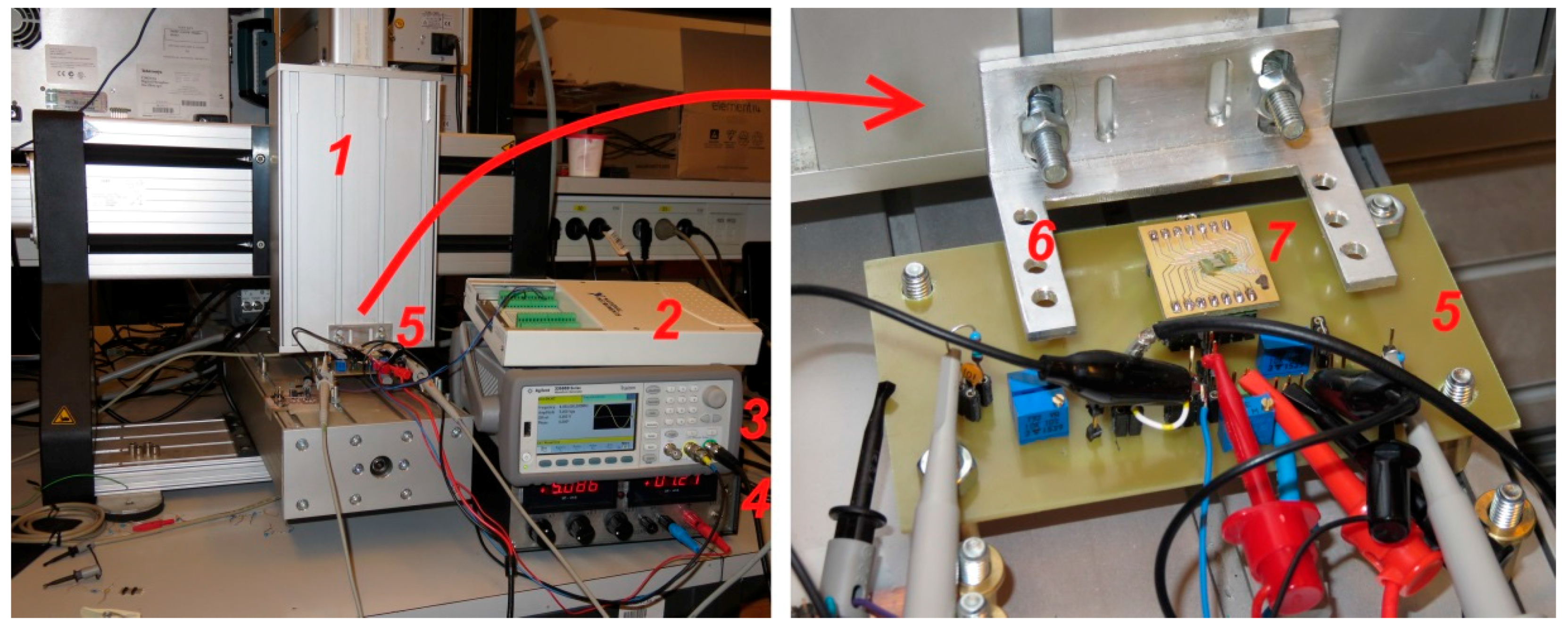
The layout of the microsystem is depicted in
Figure 11b. The silicon footprint of the analog front-end is relatively small in comparison to the area of the microtransformers. The fabricated ASIC prototype on a mounting PCB is presented in
Figure 11c. The ASIC silicon die dimensions are 2500 by 2200 µm, at a 300 µm wafer thickness. As the bonding wires are thin (several 10 µm), they can easily bend or tear in case of a contact with scale, which is highly possible. Therefore they must be protected. A protective epoxy coating is used for their encapsulation.


