
Modeling of Rate-Dependent Hysteresis Using a GPO-Based Adaptive Filter

Abstract
:1. Introduction
2. GPO and GPI Model
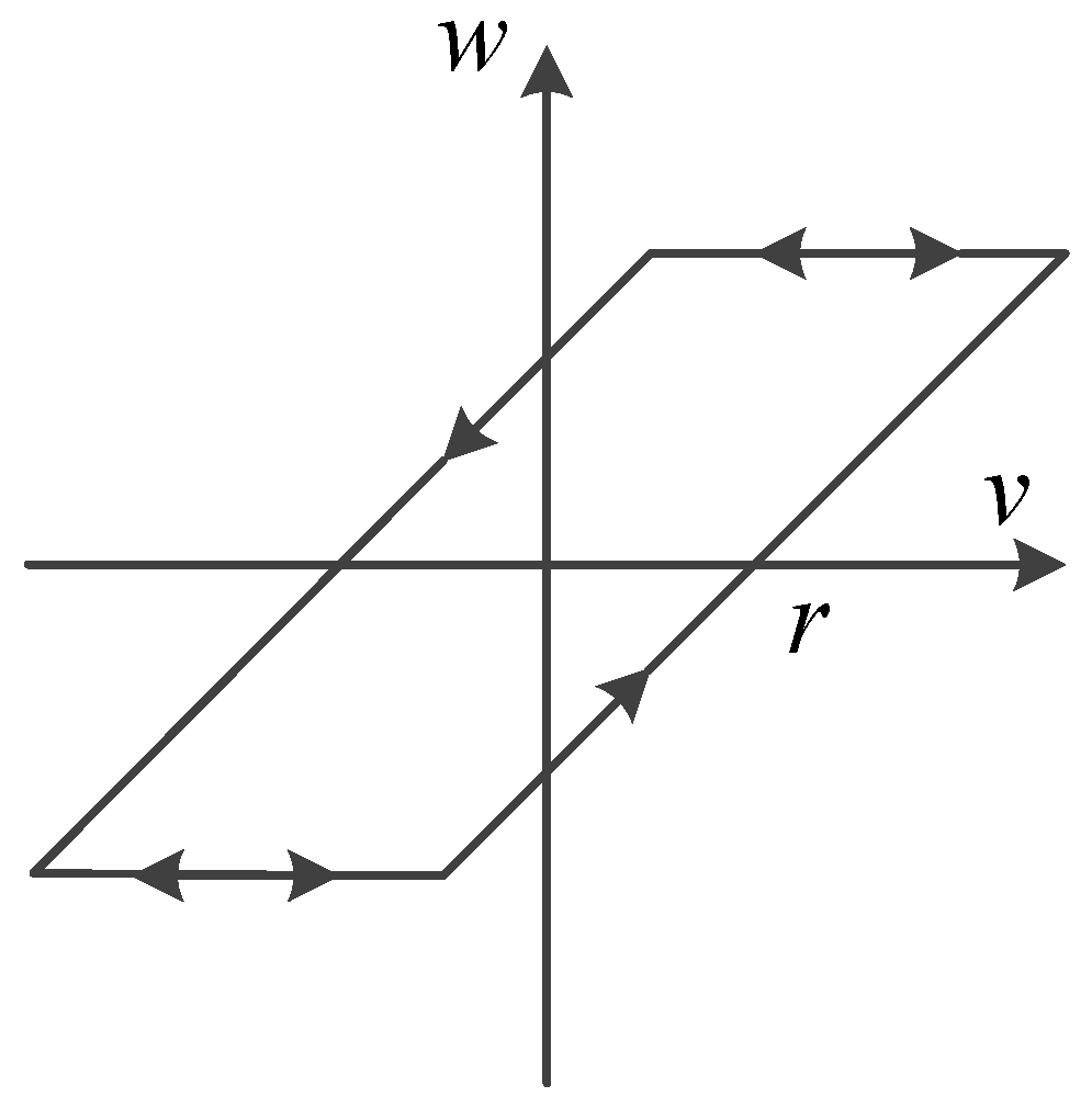
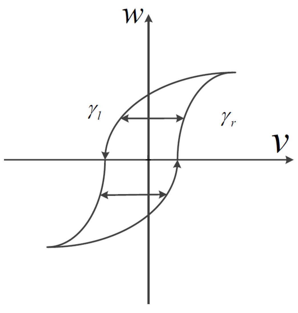
2.1. Play Operator

2.2. Generalized Play Operator

2.3. GPI Model
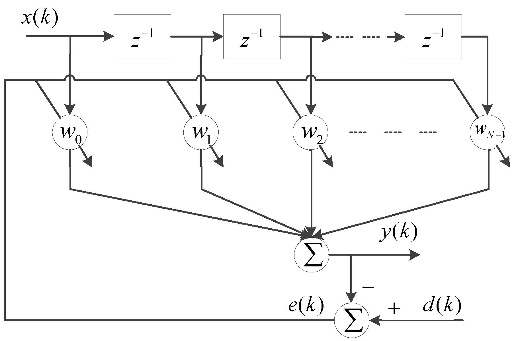
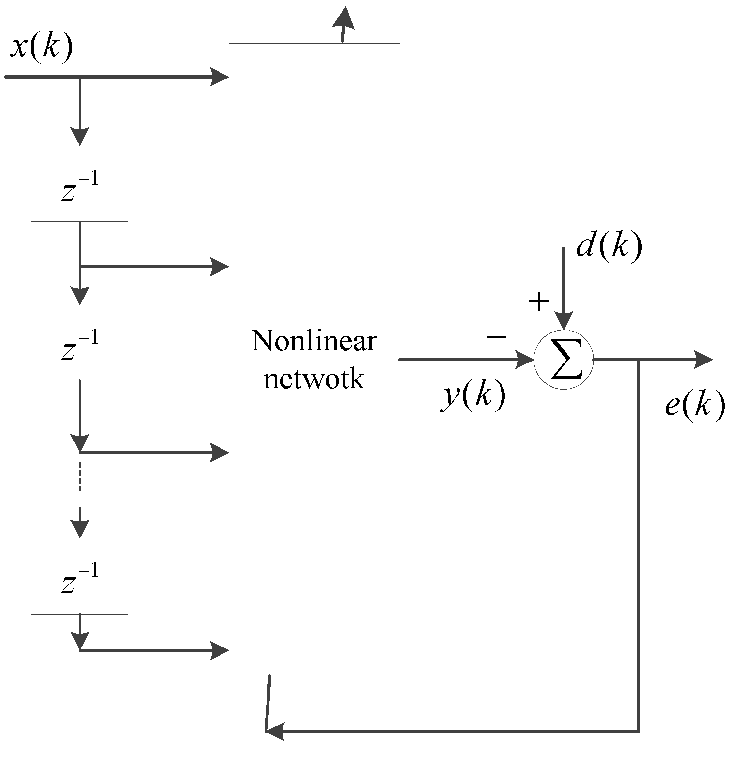
3. GPO-Based Adaptive Filter for Rate-Dependent Hysteresis Modeling
3.1. GPOs-Based Adaptive Filter
- Step 1. A sufficiently slow input signal is generated and applied to the unknown model plant; the output is measured.
- Step 2. The number of the GPOs in the GPI model is set to the same as the order of the filter N.
- Step 3. Initialize the parameters of the envelop function and the weights .
- Step 4. Calculate the thresholds using Equation (10).
- Step 5. Calculate the output of the GPI model using Equation (9).
- Step 6. Determine the parameters and , by minimization of sum-squared-error J described by Equation (11).
- Step 7. Calculate the sum-squared-error J; if J is less than tolerable error ε, then end the algorithm; else return to Step 4.
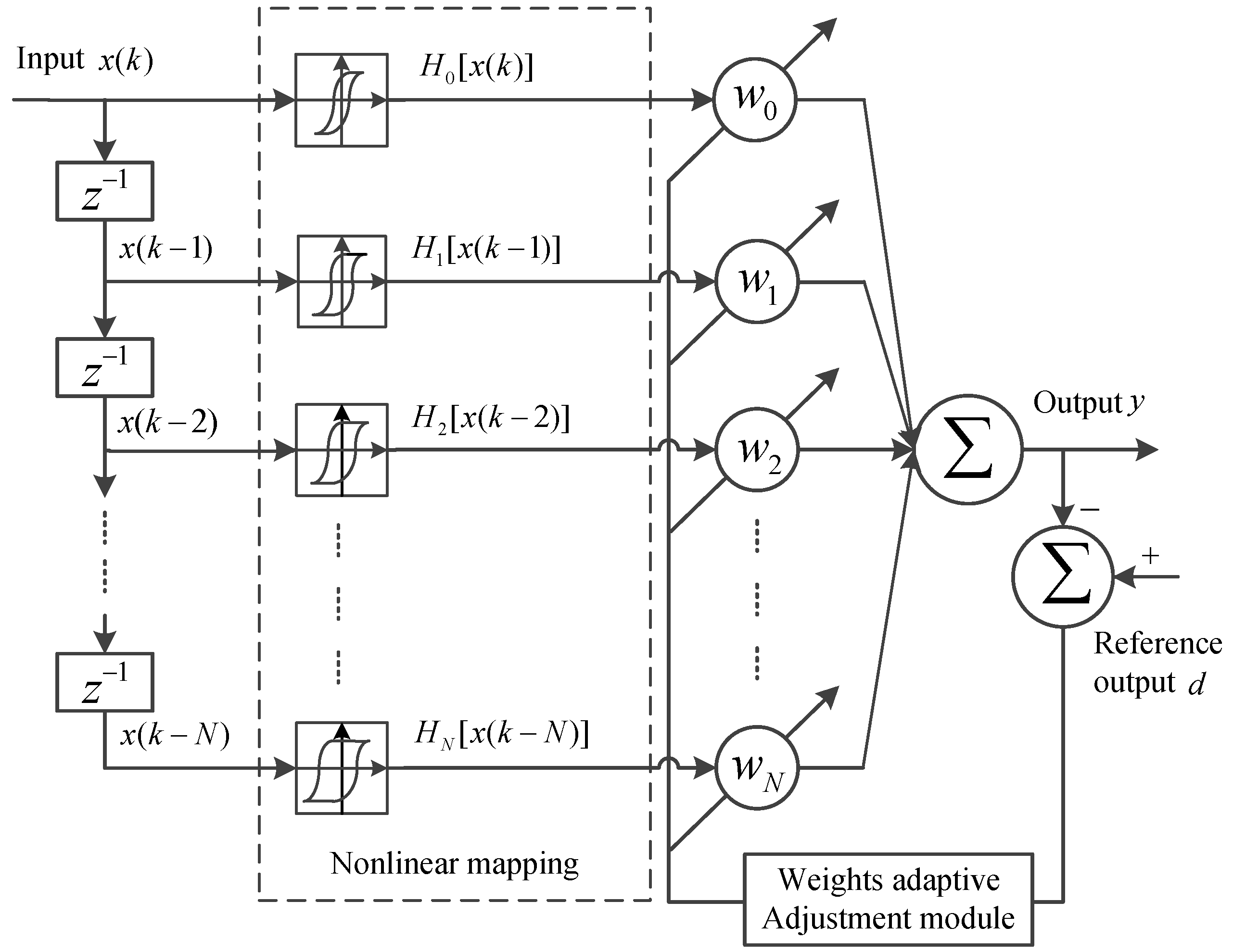
3.2. GPO LMS Algorithm
3.3. The Process of Modeling
- (1)
- Determine the order of the filter N. For the unknown model plant, Algorithm 1 is used to identify the envelop function and the threshold values of the GPOs in the filters.
- (2)
- Initialize the weight vector . Determine the convergence factor μ based on the auto-correlation matrix .
- (3)
- Construct the adaptive filter model system. Connect input signal with the input port of the model plant and the GPO-based adaptive filter. Then, connect the output signal of the model plant with the output of the GPO-based adaptive filter using a sum to calculate the error.
- (4)
- Calculate the error signal . Update the weight vector of the GPO-based adaptive filter through Equation (18).
- (5)
- Provide the next input signal and return to Step 3. Repeat the process until all input signals have been given.
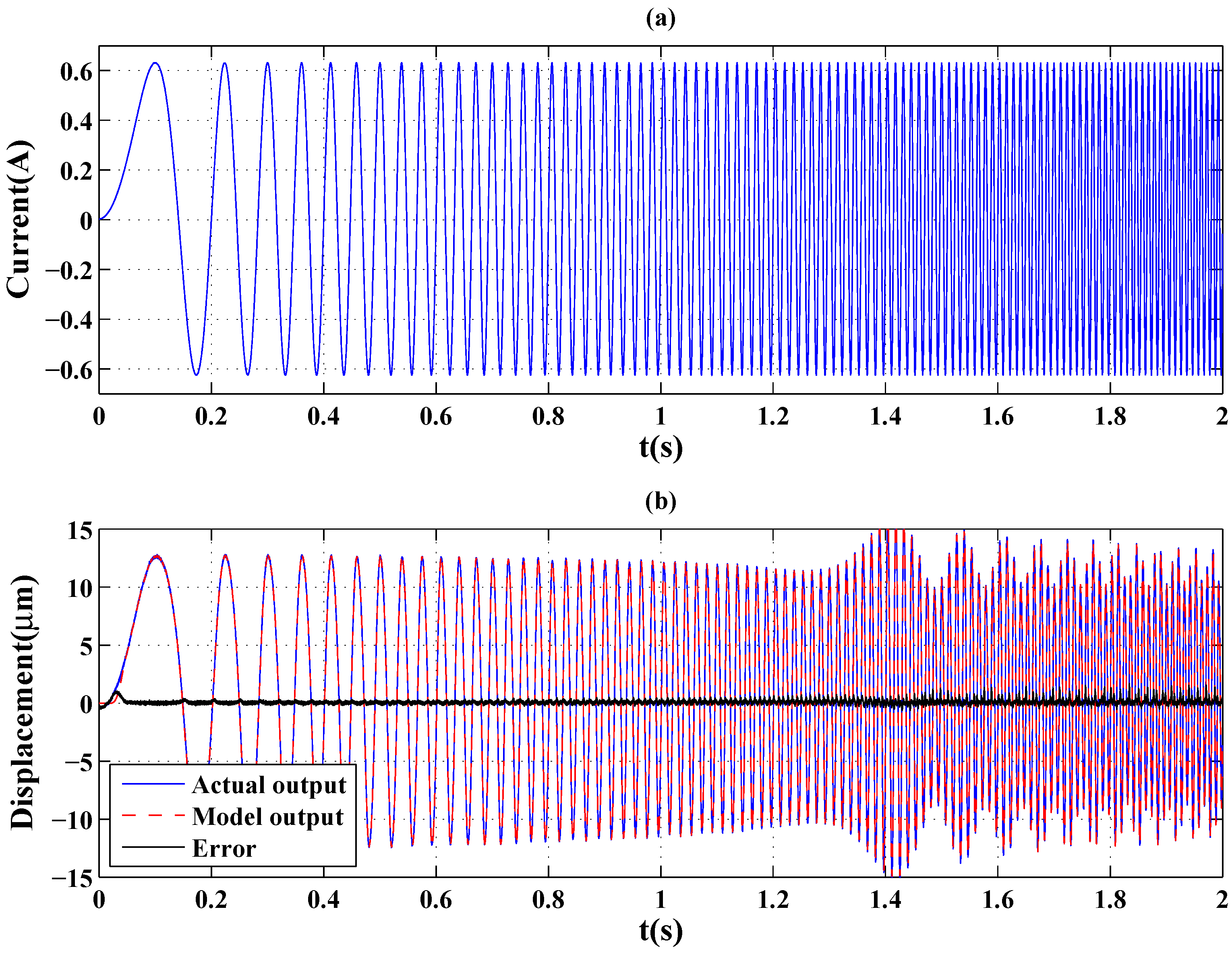
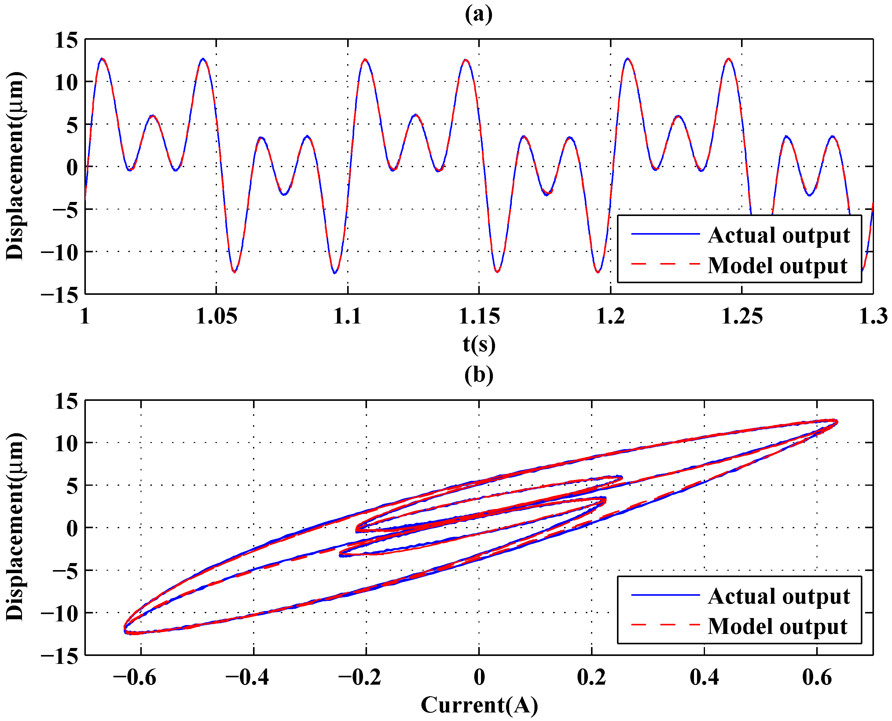
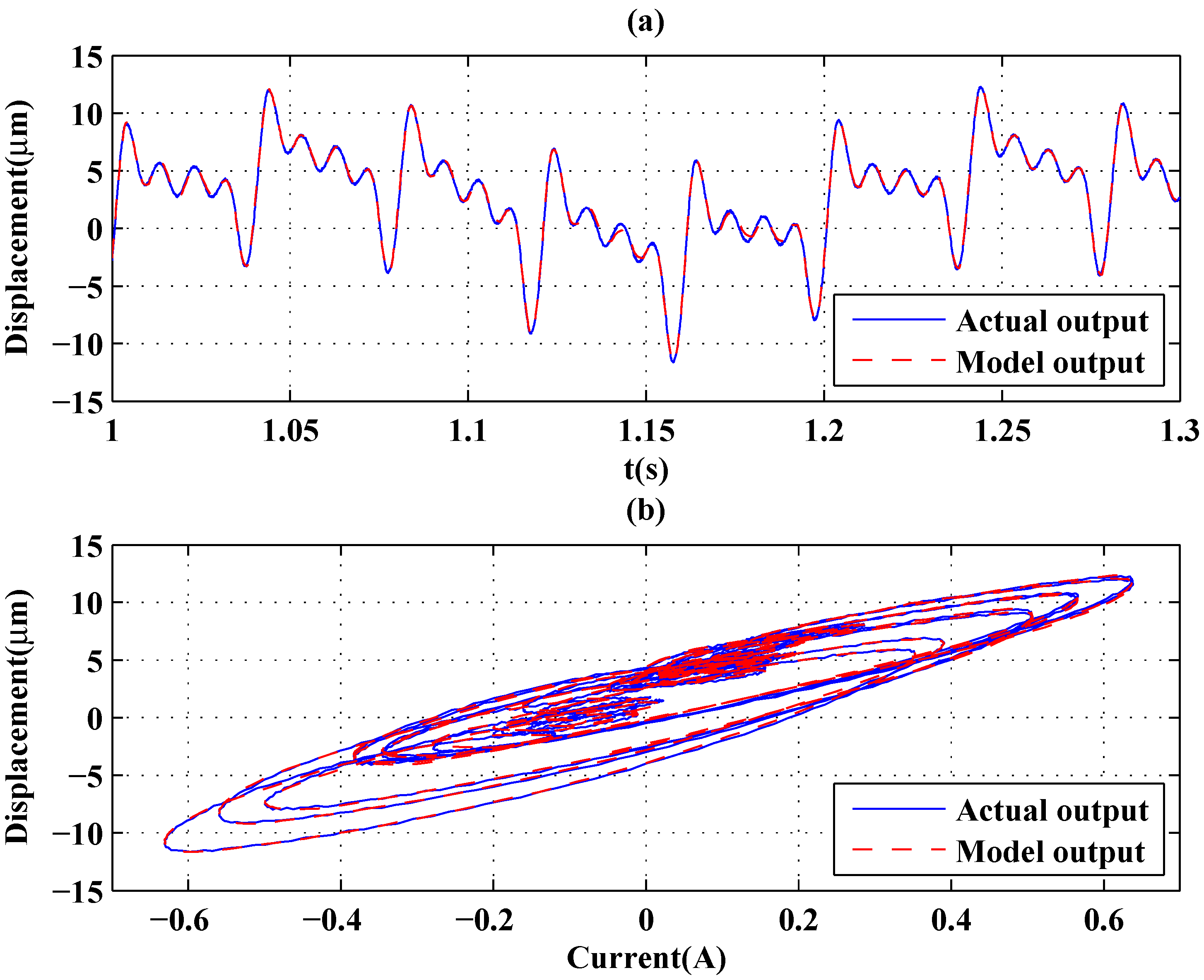
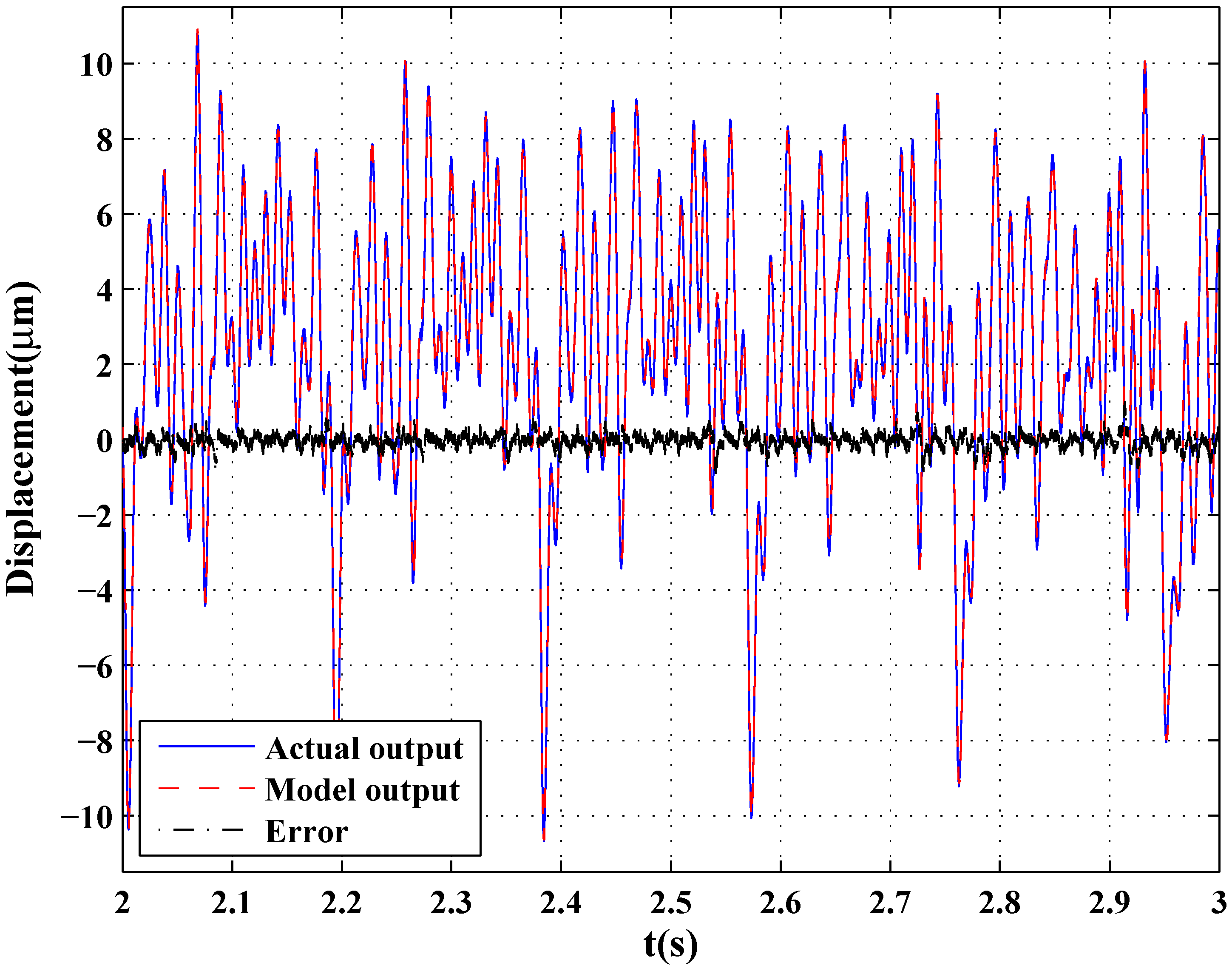
4. Model Validation and Experimental Results


| Input | GPOs-Based | Backlash | Volterra | Delayed | |
|---|---|---|---|---|---|
| Signal | Filter | Filter | Filter | Filter | |
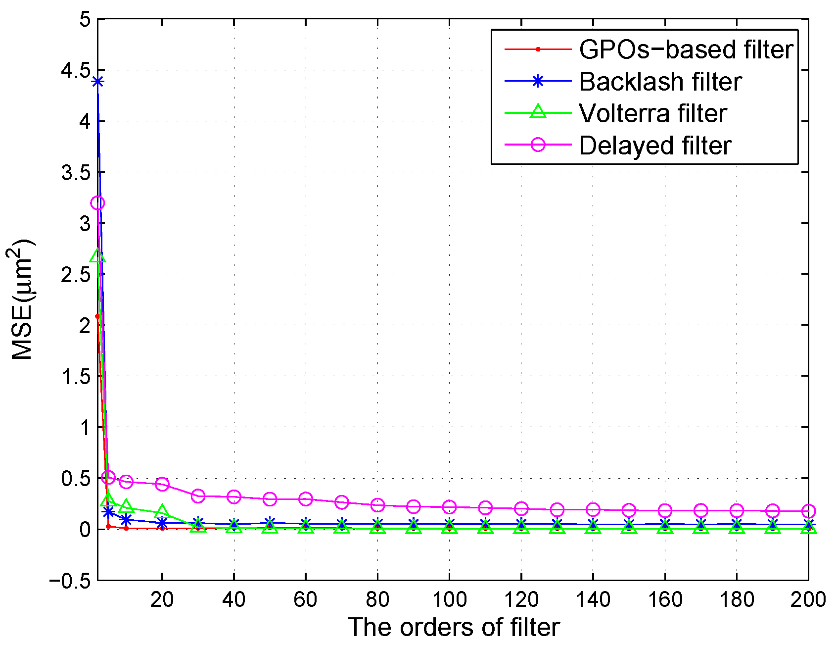
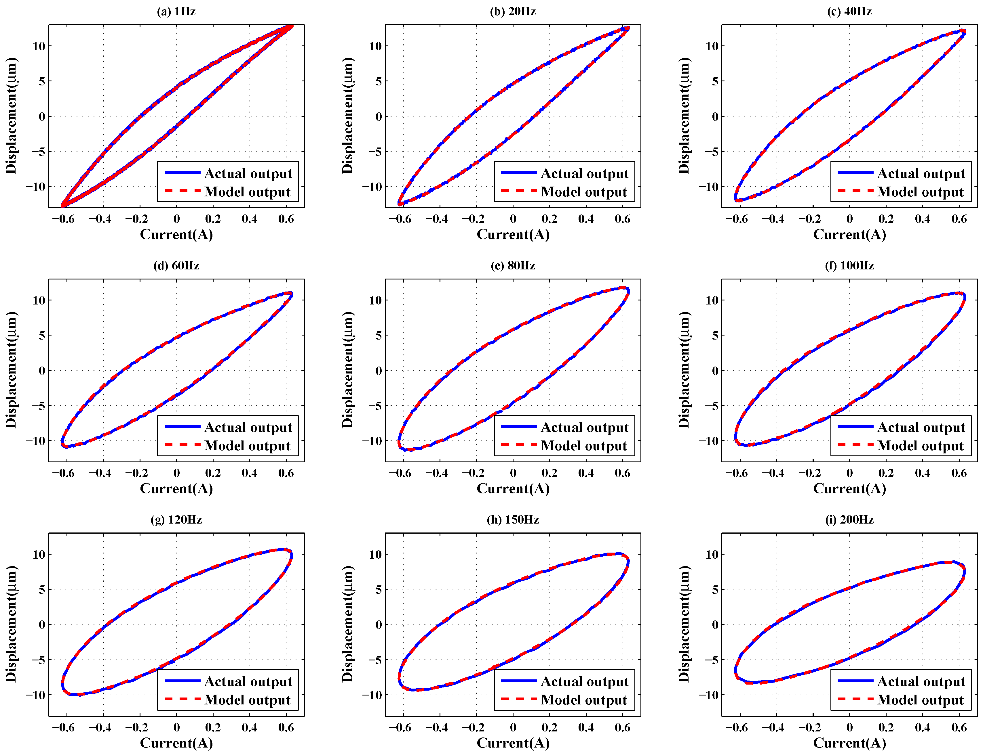
| 10 Hz sine wave | MSE (μ) | 0.0094 | 0.4248 | 1.1847 | 0.2880 |
| RE | 0.0106 | 0.0711 | 0.1187 | 0.0585 | |
| 20 Hz sine wave | MSE (μ) | 0.0095 | 0.3533 | 0.5211 | 0.2882 |
| RE | 0.0108 | 0.0658 | 0.0800 | 0.0594 | |
| 40 Hz sine wave | MSE (μ) | 0.0098 | 0.3226 | 0.2256 | 0.3560 |
| RE | 0.0114 | 0.0655 | 0.0548 | 0.0688 | |
| 60 Hz sine wave | MSE (μ) | 0.0103 | 0.1811 | 0.1310 | 0.2450 |
| RE | 0.0131 | 0.0549 | 0.0466 | 0.0638 | |
| 80 Hz sine wave | MSE (μ) | 0.0122 | 0.1857 | 0.1192 | 0.3258 |
| RE | 0.0134 | 0.0523 | 0.0417 | 0.0690 | |
| 100 Hz sine wave | MSE (μ) | 0.0119 | 0.1621 | 0.0858 | 0.3168 |
| RE | 0.0141 | 0.0520 | 0.0378 | 0.0726 | |
| 120 Hz sine wave | MSE (μ) | 0.0123 | 0.1355 | 0.0476 | 0.2828 |
| RE | 0.0151 | 0.0500 | 0.0296 | 0.0723 | |
| 150 Hz sine wave | MSE (μ) | 0.0157 | 0.1163 | 0.0224 | 0.2514 |
| RE | 0.0183 | 0.0498 | 0.0218 | 0.0732 | |
| 200 Hz sine wave | MSE (μ) | 0.0221 | 0.0896 | 0.0172 | 0.2071 |
| RE | 0.0246 | 0.0495 | 0.0217 | 0.0736 |


| Input | GPO-Based | Backlash | Volterra | Delayed | |
|---|---|---|---|---|---|
| Signal | Filter | Filter | B | Filter | |
| Chirp signal | MSE (μ) | 0.0646 | 0.4356 | 0.4882 | 0.6300 |
| Figure 9a | RE | 0.0296 | 0.0769 | 0.0814 | 0.0924 |


| Input | GPOs-Based | Backlash | Volterra | Delayed | |
|---|---|---|---|---|---|
| Signal | Filter | Filter | Filter | Filter | |
| Sum of sinusoid signal | MSE (μ) | 0.0186 | 0.0430 | 1.6099 | 1.6897 |
| (10, 30, 50 Hz), Figure 10 | RE | 0.0205 | 0.0312 | 0.1910 | 0.1954 |
| Sum of sinusoid signal | MSE (μ) | 0.0351 | 0.0882 | 1.8882 | 2.2469 |
| (5, 25, 50, 75, 100 Hz), Figure 11 | RE | 0.0370 | 0.0608 | 0.2907 | 0.3069 |
| Sum of sinusoid signal | MSE (μ) | 0.0425 | 0.0939 | 1.6865 | 1.4340 |
| Figure 12 | RE | 0.0470 | 0.0699 | 0.2964 | 0.2733 |
| Input Signal | RDGPI Model | GPO-Based Filter | |
|---|---|---|---|
| 10 Hz sine wave | MSE(μ) | 1.2298 | 0.0094 |
| RE | 0.1172 | 0.0106 | |
| 20 Hz sine wave | MSE(μ) | 0.8262 | 0.0095 |
| RE | 0.0974 | 0.0108 | |
| 40 Hz sine wave | MSE(μ) | 0.7155 | 0.0098 |
| RE | 0.0945 | 0.0114 | |
| 60 Hz sine wave | MSE(μ) | 0.5148 | 0.0103 |
| RE | 0.0835 | 0.0131 | |
| 80 Hz sine wave | MSE(μ) | 0.9183 | 0.0122 |
| RE | 0.1084 | 0.0134 | |
| 100 Hz sine wave | MSE(μ) | 0.6111 | 0.0119 |
| RE | 0.1 | 0.0141 | |
| Chirp signal | MSE(μ) | 2.6650 | 0.0646 |
| RE | 0.2225 | 0.0296 | |
| Sum of sinusoid signal | MSE(μ) | 2.7005 | 0.0186 |
| (10, 30, 50 Hz) | RE | 0.2474 | 0.0205 |
| Sum of sinusoid signal | MSE(μ) | 3.3587 | 0.0351 |
| (5, 25, 50, 75, 100 Hz) | RE | 0.3850 | 0.0370 |
| Sum of sinusoid signal | MSE(μ) | 3.7751 | 0.0425 |
| Figure 9a | RE | 0.3446 | 0.0470 |
5. Conclusions
Acknowledgments
Author Contributions
Conflicts of Interest
References
- Wang, D.; Yu, P.; Wang, F.F.; Chan, H.Y.; Zhou, L.; Dong, Z.L.; Liu, L.Q.; Li, W.J. Improving atomic force microscopy imaging by a direct inverse asymmetric PI Hysteresis Model. Sensors 2015, 15, 3409–3425. [Google Scholar] [CrossRef] [PubMed]
- Lin, J.H.; Chiang, M.H. Hysteresis analysis and positioning control for a magnetic shape memory actuator. Sensors 2015, 15, 8054–8071. [Google Scholar] [CrossRef] [PubMed]
- Jile, D.C.; Atherton, D.L. Theory of ferromagnetic hysteresis. J. Magn. Magn. Mater. 1986, 61, 48–60. [Google Scholar] [CrossRef]
- Smith, R.C.; Seelecke, S.; Ounaies, Z.; Simth, J. A free energy model for hysteresis in ferroelectric materials. J. Intell. Mater. Syst. Struct. 2003, 14, 719–739. [Google Scholar] [CrossRef]
- Smith, R.C.; Ounaies, Z. A domain wall model for hysteresis in piezoelectric materials. J. Intell. Mater. Syst. Struct. 2000, 11, 62–79. [Google Scholar] [CrossRef]
- Mayergoyz, I. Mathematical Models of Hysteresis and Their Applications; Elsevier: New York, NY, USA, 2003. [Google Scholar]
- Webb, G.V.; Lagoudas, D.C.; Kurdila, A.J. Hysteresis modeling of SMA actuators for control application. J. Intell. Mater. Syst. Struct. 1998, 9, 432–448. [Google Scholar] [CrossRef]
- Visintin, A. Differential Models of Hysteresis; Springer: Berlin, Germany, 1994. [Google Scholar]
- Kuhnen, K. Modeling identification and compensation of complex hysteretic non-linearities: A modified Prandtl-Ishlinskii approach. Eur. J. Control 2003, 9, 407–418. [Google Scholar] [CrossRef]
- Janaideh, M.A.; Rakheja, S.; Su, C.Y. A generalized Prandtl-Ishlinskii model for characterizing the hysteresis and saturation nonlinearities of smart actuators. Smart Mater. Struct. 2009, 18, 1–9. [Google Scholar] [CrossRef]
- Ma, Y.H.; Mao, J.Q.; Zhang, Z. On generalized dynamic preisach operator with application to hysteresis nonlinear systems. IEEE Trans. Control Syst. Technol. 2011, 19, 1527–1533. [Google Scholar] [CrossRef]
- Mayergoyz, I. Dynamic Preisach models of hysteresis. IEEE Trans. Magn. 1988, 24, 2925–2927. [Google Scholar] [CrossRef]
- Wolf, F.; Sutor, A.; Rupitsch, S.J.; Lerch, R. Modeling and measurement of creep- and rate-dependent hysteresis in ferroelastic actuators. Sens. Actuators A Phys. 2011, 172, 245–252. [Google Scholar] [CrossRef]
- Wolf, F.; Sutor, A.; Rupitsch, S.J.; Lerch, R. Modeling and measurement of hysteresis of ferroelectric actuators considering time-dependent behavior. Procedia Eng. 2010, 5, 87–90. [Google Scholar] [CrossRef]
- Ang, W.T.; Khosla, P.K.; Riviere, C.N. Feedforward controller with inverse rate-dependent model for piezoelectric actuators in trajectory-tracking applications. IEEE/ASME Trans. Mechatron. 2007, 12, 134–142. [Google Scholar] [CrossRef]
- Janaideh, M.A.; Su, C.Y.; Rakheja, S. Development of the rate-dependent Prandtl-Ishlinskii model for smart actuators. Smart Mater. Struct. 2008, 17, 1–12. [Google Scholar] [CrossRef]
- Tan, X.B.; Baras, J.S. Modeling and control of hysteresis in Magentostrictive actuators. Automatica 2004, 40, 1469–1480. [Google Scholar] [CrossRef]
- Zhang, Z.; Mao, J.Q. Modeling rate-dependent hysteresis for magnetostrictive actuator. Mat. Sci. Forum 2007, 546–549, 2251–2256. [Google Scholar]
- Deng, L.; Tan, Y.H. Diagonal recurrent neural network with modified backlash operators for modeling of rate-dependent hysteresis in piezoelectric actuators. Sens. Actuators A Phys. 2008, 148, 259–270. [Google Scholar] [CrossRef]
- Zhang, X.L.; Tan, Y.H.; Su, M.Y. Modeling of hysteresis in piezoelectric actuator using neural networks. Mech. Syst. Signal Process. 2009, 23, 2699–2711. [Google Scholar] [CrossRef]
- Mao, J.Q.; Ding, H.S. Intelligent modeling and control for nonlinear systems with rate-dependent hysteresis. Sci. China Ser. F Inf. Sci. 2009, 52, 656–673. [Google Scholar] [CrossRef]
- Xu, Q.S.; Wong, P.K. Hysteresis modeling and compensation of a piezostage using least squares support vector machines. Mechatronics 2011, 21, 1239–1251. [Google Scholar] [CrossRef]
- Widrow, B.; Stearns, S.D. Adaptive Signal Processing; Prentice-Hall: Englewood Cliffs, NJ, USA, 1985. [Google Scholar]
- Widrow, B.; Walach, E. Adaptive Inverse Control: A Signal Processing Approach; John Wiley & Sons: Hoboken, NJ, USA, 2007. [Google Scholar]
- Liu, X.D.; Wang, Y.; Geng, J.; Chen, Z. Modeling of hysteresis in piezoelectric actuator based on adaptive filter. Sens. Actuators A Phys. 2013, 189, 420–428. [Google Scholar] [CrossRef]
- Diniz Paulo, S.R. Adaptive Filtering Algorithms and Practical Implementation; Springer: New York, NY, USA, 2008. [Google Scholar]
- Irving, A.D. Dynamical hysteresis in communications: A Volterra functional approach. IET Signal Process. 2008, 2, 75–86. [Google Scholar] [CrossRef]
- Zhao, S.K.; Jones, D.L.; Khoo, S.; Man, Z.H. New Variable Step-Sizes Minimizing Mean-Square Deviation for the LMS-Type Algorithms. Circuits Syst. Signal Process. 2014, 33, 2251–2265. [Google Scholar] [CrossRef]
- Ge, H.M.; Zhao, W.W. Improved variable step-size and variable parameters LMS adaptive filtering algorithm. Sens. Transducers 2013, 158, 369–373. [Google Scholar]
- Batista, E.L.O.; Tobias, O.J.; Seara, R. A sparse-interpolated scheme for implementing adaptive Volterra filters. IEEE Trans. Signal Process. 2010, 58, 2022–2035. [Google Scholar] [CrossRef]
- Batista, E.L.O.; Seara, R. A fully LMS/NLMS adaptive scheme applied to sparse-interpolated Volterra filters with removed boundary effect. Signal Process. 2012, 92, 2381–2393. [Google Scholar] [CrossRef]
- Janaideh, M.A.; Su, C.Y.; Rakheja, S. Compensation of rate-dependent hysteresis nonlinearities in a piezo micro-positioning stage. In Proceedings of the 2010 IEEE International Conference on Robotics and Automation, Anchorage, AK, USA, 3–8 May 2010; pp. 512–517.
© 2016 by the authors; licensee MDPI, Basel, Switzerland. This article is an open access article distributed under the terms and conditions of the Creative Commons by Attribution (CC-BY) license (http://creativecommons.org/licenses/by/4.0/).
Share and Cite
Zhang, Z.; Ma, Y. Modeling of Rate-Dependent Hysteresis Using a GPO-Based Adaptive Filter. Sensors 2016, 16, 205. https://doi.org/10.3390/s16020205
Zhang Z, Ma Y. Modeling of Rate-Dependent Hysteresis Using a GPO-Based Adaptive Filter. Sensors. 2016; 16(2):205. https://doi.org/10.3390/s16020205
Chicago/Turabian StyleZhang, Zhen, and Yaopeng Ma. 2016. "Modeling of Rate-Dependent Hysteresis Using a GPO-Based Adaptive Filter" Sensors 16, no. 2: 205. https://doi.org/10.3390/s16020205
APA StyleZhang, Z., & Ma, Y. (2016). Modeling of Rate-Dependent Hysteresis Using a GPO-Based Adaptive Filter. Sensors, 16(2), 205. https://doi.org/10.3390/s16020205