1. Introduction
In the rotating machinery, gearboxes are widely used to transmit power from the prime mover to the load. If any failure occurs in the gearbox, it may interrupt normal machine operation and endanger users. Consequently, it is of great significance to develop a reliable and accurate intelligent system to diagnose the main components of the gearbox, such as gears and bearings. There are two main challenges in gearbox diagnosis. One is the existence of simultaneous faults, that is, multiple single faults that appear concurrently. The other is that no unique sensor can detect all the machine faults. To accurately detect more faults, many kinds of sensors and signals may be involved at the same time. However, it is difficult to analyze different kinds of signals simultaneously and make a decision. In the [
1,
2,
3,
4,
5,
6,
7], various gearbox diagnostic systems have been proposed. In these systems, the fault diagnosis procedures are mainly divided into two stages: (1) signal processing and (2) fault identification/classification.
The existing problems in signal processing of these systems are that the signals usually contain high-dimensional data and suffer from background noise interference, which degenerates the accuracy and fault identification time. Besides, the gearbox usually has many rotating components working together, such as bearings, gears and spindles, so the diagnosis of the gearbox is a simultaneous fault problem. In traditional gearbox fault diagnostic methods, simultaneous faults are usually considered as an independent label for the classifier, which will result in a high cost in acquiring exponentially increased simultaneous fault signals. For example, with
d single-faults (labels) and one normal condition, there are 2
d − (
d + 1) artificial simultaneous fault labels [
8,
9,
10]. To solve this problem, an effective signal de-noising method and a proper feature extraction technique which can find the single fault pattern features in simultaneous fault patterns are studied together.
Currently, some methods, including spectral subtraction, least squares, and wavelet threshold methods, are widely used for signal de-nosing [
11,
12]. In order to effectively de-noise the non-stationary signals of a gearbox, a soft threshold method based on the discrete wavelet transform (DWT) is adopted in this study due to its popularity.
References [
8,
9,
10] reported that a simultaneous fault symptom can be identified by analyzing the single fault patterns only if the classifier is trained by using a proper feature extraction technique, so that it can save a lot of resources to collect a large combination of simultaneous fault training data. Existing techniques to select a proper feature extraction technique are reviewed here. At present, there exist many methods to extract features from fault signals, such as Fourier transform, short time Fourier transform, and wavelet transform. The Fourier transform is only suitable for analyzing stationary signals. However, the signals of rotating gears and bearings are non-stationary, which makes the Fourier transform unsuitable for this application. The time-frequency analysis methods, such as short time Fourier transform (STFT) and wavelet transform, can process non-stationary signals, but they all have limitations. STFT has a limitation in non-stationary signal processing because of its use of a fixed time window which makes it impossible to achieve good resolution in the time and frequency domains at the same time. The drawback of the wavelet transform is that it suffers from the effect of the energy leakage because any signal which does not well correlate with the shape of wavelet basis function will be masked or completely ignored. In contrast to STFT and the wavelet transform, the Hilbert-Huang transform (H-HT) is the latest time-frequency signal processing technique to analyze nonlinear and non-stationary signals. The first step of a typical H-HT process is to employ the empirical mode decomposition (EMD) algorithm to decompose a complicated signal into a series of intrinsic mode functions (IMFs), which contains the local characteristics of the original signal at different time scales, and then a Hilbert transform is applied to each intrinsic mode function (IMF) for Hilbert spectrum analysis. The high time-frequency resolution of the H-HT method can effectively describe the rules of the changing frequency compositions with time, which is a good approach for analyzing non-stationary signals. Even though H-HT has been applied to many applications, particularly in fault detection and diagnosis [
13,
14], it has some disadvantages: (1) the issue of mode mixing; and (2) the redundant intrinsic mode functions easily appear at low frequency, which can cause the distortion of the processed result [
15]. To overcome these disadvantages, this study applies ensemble empirical mode decomposition (EEMD), an improved EMD method, to deal with the mode mixing problem, and uses the correlation coefficient method to eliminate the redundant IMFs. The EEMD-based H-HT is hereafter refered to as HHT. It is well-known that different fault conditions show different amplitude- and phase-frequency characteristics in the frequency domain. In other words, fault signal energies in some frequency bands may be enhanced, while the others are restrained. It is reasonable to assume that there are certain corresponding relationships between the signal energy changes in the frequency bands and the fault phenomena. Therefore, on the basis of HHT, energy patterns of the selected intrinsic mode function components are considered in this study to further extract representative fault features from the gearbox vibration and sound signals.
In [
1,
3,
5], most of the existing fault classification systems for the rotating machinery are constructed by a single classifier which is trained based on one type of signal. However, a single classifier-based fault diagnostic system may not give reliable fault diagnostic results due to the fact that a universal classifier is difficult to develop, especially when the data available for training the classifier are not abundant. Furthermore, a single classifier can only be trained by one type of signal. Obviously, only one type of signal may not be able to cover all the faults. To let a fault classification system generate more reliable diagnostic result and diagnose more faults, this paper proposes a new probabilistic committee machine (PCM) to combine the diagnostic results from vibration and sound signals. From the gearbox point of view, vibration and sound signals are usually used to identify the faults because those signals are easily acquired and highly related to the conditions of the gearbox [
16,
17,
18,
19,
20,
21]. The committee machine concept involves combining results acquired by individual classifiers so as to obtain a group decision that is superior to any individual classifier acting alone [
22,
23,
24], because a group decision is usually better than a single person’s decision.
Moreover, a proper classifier must be able to offer the probabilities of all possible faults so that the user can at least trace the other possible faults according to the rank of their probabilities when the fault(s) predicted by the classifier are incorrect. Therefore, it is logical to employ a probabilistic classifier for each member in the committee machine for simultaneous-fault diagnosis of the gearbox. Currently, there are two common probabilistic classifiers, the probabilistic neural network (PNN) [
25,
26] and relevance vector machine (RVM) [
27,
28] available in the relevant literature. The main drawback of PNN lies in the limited number of inputs because the complexity of the network and the training time are heavily related to the number of inputs. Hence, RVM is selected as a probabilistic classifier to build each committee member in this study. Generally, the aforementioned probabilistic classifiers are suitable to solve the binary classification. Nevertheless, most of the practical applications are multi-class classification problems. One-
versus-all strategy is usually employed to fix the multi-class classification problem. However, this strategy does not consider the correlation between every pair of faults or labels, which was verified to produce a large region of indecision [
29]. To solve the multi-class classification problem effectively and generate a probability, a suitable pairwise coupling strategy is adopted for the above probabilistic classifiers to generate a pairwise-coupled probabilistic neural network (PCPNN) and pairwise-coupled relevance vector machine (PCRVM).
After determining the methods of signal de-noising, feature extraction and committee members, there are still two major factors, the decision threshold
ε and member weight
w, affecting the system accuracy in the proposed framework. The probabilistic committee machine only produces the probability of occurrence of each fault. To determine the occurrence of the faults, a decision threshold must be applied to those probabilities (e.g., output probabilistic vector
P = [0.35, 0.58, 0.48, 0.83], if
ε = 0.5, fault labels (2, 4) are considered as faults). Besides, different committee members usually have various reliabilities, so a fair committee machine should assign different weights to their committee members. Hence, an efficient searching algorithm, particle swarm optimization (PSO) [
30,
31], to determine optimal member weights and decision threshold is considered in the proposed framework. Finally, a fair measure,
F-measure, is employed to evaluate the performance of the proposed diagnostic framework.
In a nutshell, this paper proposes a new framework which can diagnose simultaneous faults in the gearbox while the framework is trained using only single-fault patterns. Besides, the proposed framework can provide probabilities of all possible faults to users to trace the other possible faults according to the rank of probabilities when the diagnostic result is incorrect. Furthermore, the proposed framework can generate a more reliable diagnostic result and diagnose more faults by simultaneously analyzing vibration and sound signals. Even though the authors also proposed a similar framework for simultaneous-fault diagnosis of automotive engines in [
21], the proposed framework is targeted at the gearbox system. Moreover, the signal patterns used in this application are totally different from the ones in [
21]. The proposed framework is designed based on vibration and sound signals rather than air ratio, ignition and acoustic signals in the previous framework. Besides, the engine signals acquired in [
21] do not consider the issue of background noise which can degenerate the accuracy of the diagnostic system. Furthermore, the feature extraction and selection methods rely on EMD + domain knowledge and sample entropy, which are old, time-consuming, out of support from reference materials, and have a risk of mode-mixing. Finally, the objective function in [
21] is not well-defined that cannot achieve good diagnostic accuracy. Therefore, the framework in [
21] cannot be directly applied and is modified significantly to suit for the gearbox, particularly in the phases of data processing and feature selection.
Table 1 summarizes the differences between the diagnostic framework in [
21] and this study.
Table 1.
Differences of diagnostic framework between reference [
21] and this study.
Table 1.
Differences of diagnostic framework between reference [21] and this study.
| Differences | Reference [21] | Present Study |
|---|
| Application | Automotive engine | Gearbox |
| Signal patterns | Air ratio, ignition and acoustic signals | Vibration and sound signals |
| Signal de-noising | None | Wavelet threshold |
| Feature extraction | EMD and domain knowledge | EEMD-based Hilbert-Huang transform and energy pattern |
| Feature selection (IMF selection) | Value of sample entropy | Correlation coefficient |
| Objective function | Fme 0.925 ± 0.025 | Fme 0.9 |
This paper is organized as follows:
Section 2 presents the proposed framework and related techniques. The experimental setup and data per-processing are discussed in
Section 3.
Section 4 discusses the experimental results and a comparison with other approaches. Finally, conclusions are given in
Section 5.
2. Proposed Framework
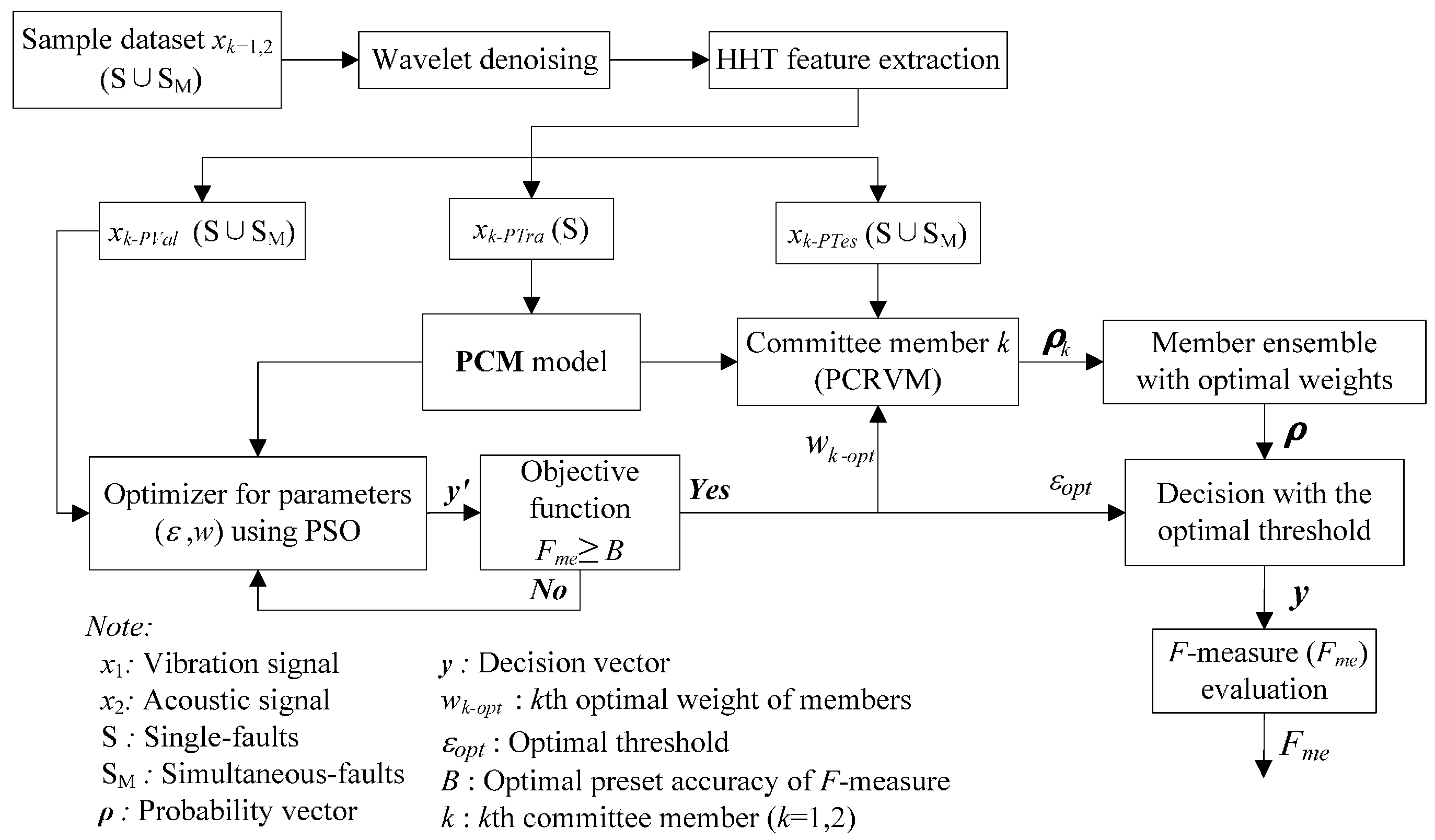
The proposed PCM framework for the gearbox simultaneous-fault diagnosis, evaluation approach and its construction method are illustrated in
Figure 1. The framework consists of four sub-modules: (1) data processing; (2) probabilistic committee machine; (3) parameter optimization; and (4) performance evaluation. The details of the four sub-modules in the framework are discussed in the following sub-sections.
Figure 1.
Proposed framework of gearbox simultaneous-fault diagnosis using probabilistic committee machine.
Figure 1.
Proposed framework of gearbox simultaneous-fault diagnosis using probabilistic committee machine.
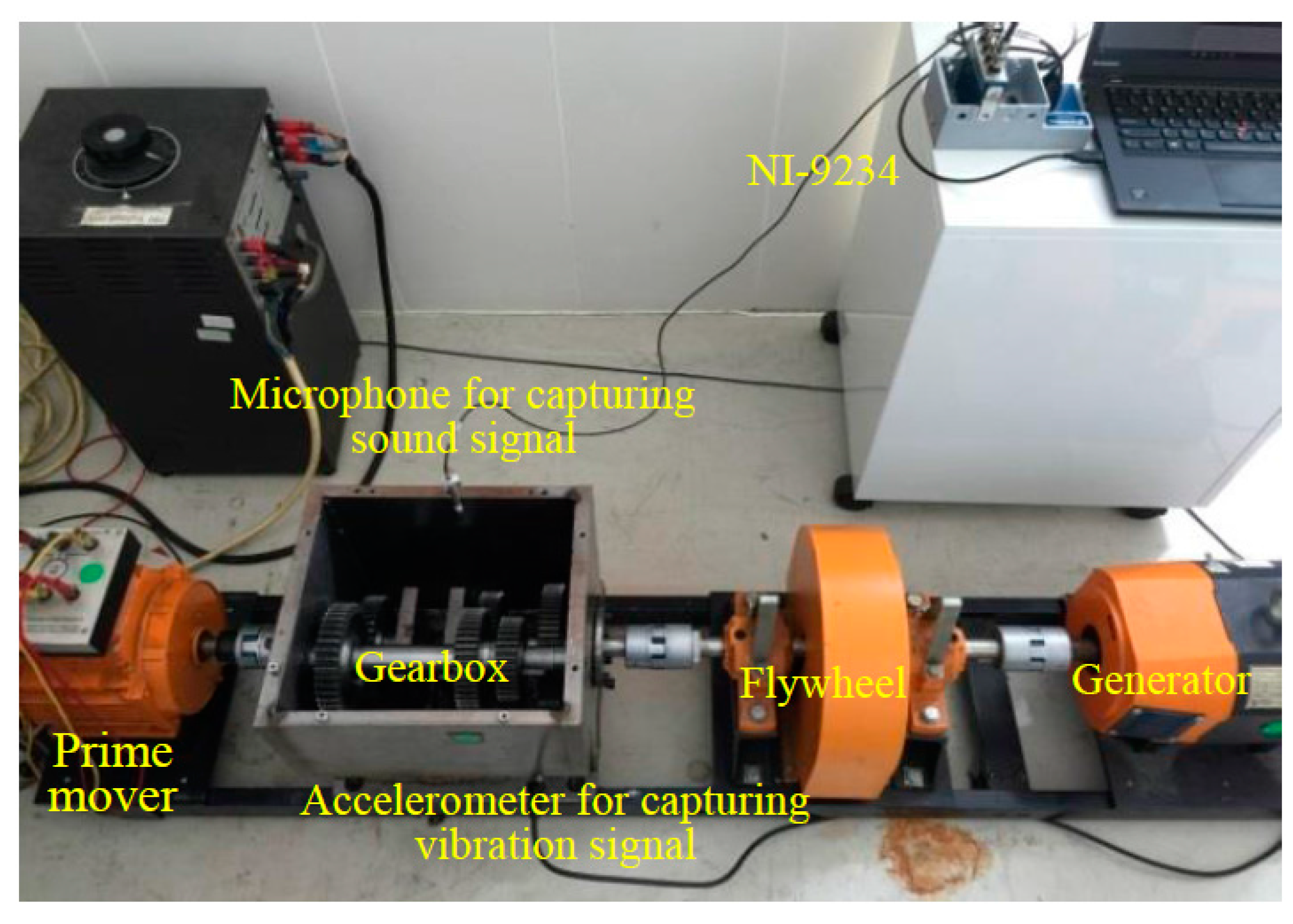
In this case study, signal features are extracted from two kinds of signals xk (k = 1, 2), including the vibration and sound signals, which are denoted as x1 and x2, respectively. Taking the vibration signal as an example, the signal x1, including both single-fault patterns (S) and simultaneous-fault patterns (SM), goes through de-noising and feature extraction. After the data processing, the processed dataset is divided into three independent groups, including validation dataset, training dataset, and test dataset which are named as x1-PTra, x1-PVal, and x1-PTes, respectively. The x1-PVal and x1-PTes involve the combination of both single-fault patterns and simultaneous-fault patterns, while x1-PTra contains the single-fault patterns only. The divided datasets are used to train, validate, and test the proposed framework.
2.1. Data Processing
2.1.1. Signal De-Noising
The acquired signals are display interference from the background noise. To decrease the interference, the acquired signals have to be de-noised. A discrete wavelet transform (DWT) technique, which is an effective de-noising technique for non-stationary signals [
11,
13], is selected in this paper. The DWT can be defined as:
where
s and
R are integers, 2
s and 2
sR represent the scale and translation parameters respectively,
Ψ represents the mother wavelet and
Ψ* is the complex conjugate of
Ψ. The original signal in time-domain
xk =
x(
t) goes through a set of low pass and high pass filters emerging as low frequency (approximations,
a*) and high frequency (details,
) signals. Therefore, the original signal
x(
t) can be written as:
The DWT-based de-noising technique is performed in three steps: (1) signal decomposition; (2) determination of the threshold and nonlinear shrinking coefficients; and (3) signal reconstruction. In the family of mother wavelets, the Daubechies wavelet (Db) is the most popular one and hence it is employed in this study. Moreover, the soft threshold signal is defined as
, if
, and otherwise is 0, where
T denotes a universal threshold that equals to
. The detail of the de-noising is described in
Section 3.2.
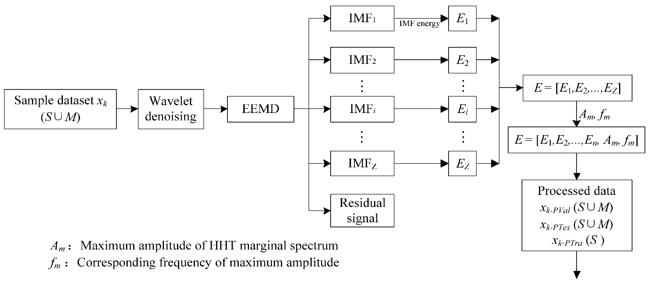
2.1.2. Feature Extraction Based on Hilbert-Huang Transform
The Hilbert-Huang transform (HHT) mentioned in this paper combines EEMD and the Hilbert transform. EEMD defines the true IMFs as the ensemble mean of trails, which consist of the decomposition of the signal plus a white noise of finite amplitude. In most cases, the range of the standard deviation is from 0.1 to 0.4 [
32]. The EEMD algorithm [
33] is given as follows:
- (1)
Initialize the number of ensemble J, the amplitude of the added white noise, and set j = 1.
- (2)
Perform the
jth trial on the white noise-added signal. A white noise series with the given amplitude is added to the investigated signal:
where
nj represents the
jth added white noise series,
x(t)’ is the de-noised signal and
x’j denotes the noise-added signal of the
jth trial.
- (3)
With the EMD method, the noise-added signal xj is decomposed into I IMFs as ci,j(t), for i = 1, 2, …, I, where ci,j represents the ith IMF of the jth trial, and I is the number of IMFs.
- (4)
If j < J then let j = j + 1. Repeat Steps 2 and 3 again and again, but with different white noise series each time until j = J.
- (5)
Calculate the ensemble mean
of
J trials for each IMF:
- (6)
Report the mean of the I IMFs as the final IMFs.
Applying the Hilbert transform to each IMF, and calculating the instantaneous frequency
(
t) and amplitude
Aj(
t), the Hilbert spectrum of
x(
t)’,
, is then calculated by the following equation:
Accordingly, the marginal spectrum of Hilbert-Huang transform,
h(
), can be defined by an integrated spectrum with respect to time,
t,
i.e.:
where
h(
) reflects the amplitude changing with frequency in the entire frequency range, and
l is the length of the signal
x(
t)’. The instantaneous frequency of IMF, which is obtained from the Hilbert transform, is well-localized in the time-frequency domain and reveals important characteristics of the signal.
2.2. Probabilistic Committee Machine
PCM is a group decision method which combines the results from the individual classifier and generates superior performance to any of the individual classifier acting alone. As mentioned previously, RVM is selected for constructing the probabilistic fault classifier. To solve the multi-label classification problem effectively, RVM adopts a pairwise coupling strategy which is named PCRVM. Moreover, a new ensemble method is proposed to combine the output of each committee member. In the proposed ensemble method, the committee members should be assigned suitable weights since every member/classifier in the group usually has its own strength. The details of PCRVM algorithm and ensemble method are described in the following sections.
2.2.1. Relevance Vector Machine
RVM is a statistical learning method utilizing Bayesian learning framework and popular kernels. In this research, predicting the posterior probability of each fault
tn for unseen symptoms
f is conducted by RVM based on experimental data. Given a set of training data (
f,
t) = {
fn,
tn},
n = 1 to
N,
tn {0, 1}, and
N is the number of training data. It follows the statistical convention and generalizes the linear model by applying the logistic sigmoid function
to the predicted decision y(
f) and adopting the Bernoulli distribution for
, the likelihood of the data is written as:
where
is a weight vector and
K is a kernel function. In the open literatures, three kinds of kernel functions, radial basis function (RBF), polynomial, and Gaussian kernels, are available. Among these kernel functions, Gaussian kernel is the most popular kernel function in RVM to deal with the issue of classification for industrial applications [
34].
The optimal weight vector
for the given dataset needs to be computed so as to maximize the probability
P(
|
t,
F,
α)
P(
t|
F,
)
P(
|
α), with
α = [α0, α1, …, αN] a vector of
N + 1 hyperparameters. However, the weights cannot be determined analytically. Thus, the following approximation procedure is chosen, which is based on Laplace’s method:
- (1)
For the current fixed values of
α, the most probable weights
are found. Since
P(
|
t,
F,
α)
P(
t|
F,
)
P(
|
α), this step is equivalent to the following maximization.
where
.
- (2)
Laplace’s method is simply a Gaussian approximation to the log-posterior around the mode of the weights
. Equation (8) is differentiated twice to give:
where
is a diagonal matrix with
and
is a
N × (
N + 1) design matrix with
and
,
n = 1 to
N, and
m = 1 to
N + 1. By inverting Equation (9), the covariance matrix
can be obtained.
- (3)
The hyperparameter vector
α is updated using an iterative re-estimation equation. Firstly,
αi is randomly guessed, then
is calculated, where
is the
ith diagonal element of the covariance matrix
Then,
αi is re-estimated as follows:
where
. The first step is to set
and then
and
are re-estimated again until convergence. Finally,
is set, so that the classification model
is obtained.
2.2.2. Pairwise-Coupled Relevance Vector Machine as Committee Member
The traditional machine learning methods are designed only for the issue of binary classification, in which the output is either positive (+1) or negative (−1). However, most practical problems are multi-classification as well as probabilistic output. Usually, one-
versus-all is employed to deal with multi-classification problems. The one-
versus-all strategy constructs a group of classifiers
lclass = [
C1,
C2, …,
Cd] in a
d-label classification problem. The one-
versus-all strategy is simple and easy to implement, however, it generally gives a poor result [
29,
35] since one-
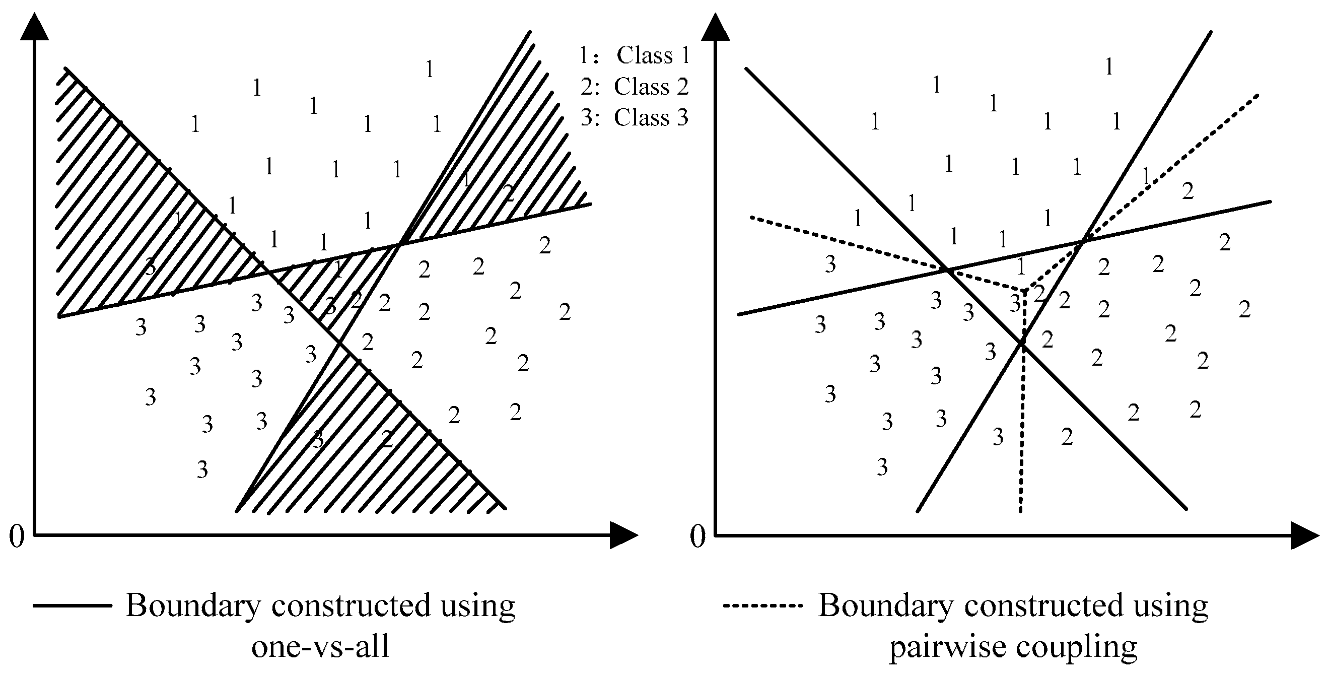
versus-all does not consider the pairwise correlations which causes a much larger indecisive region than the pairwise coupling strategy (using one-
versus-one) as showed in
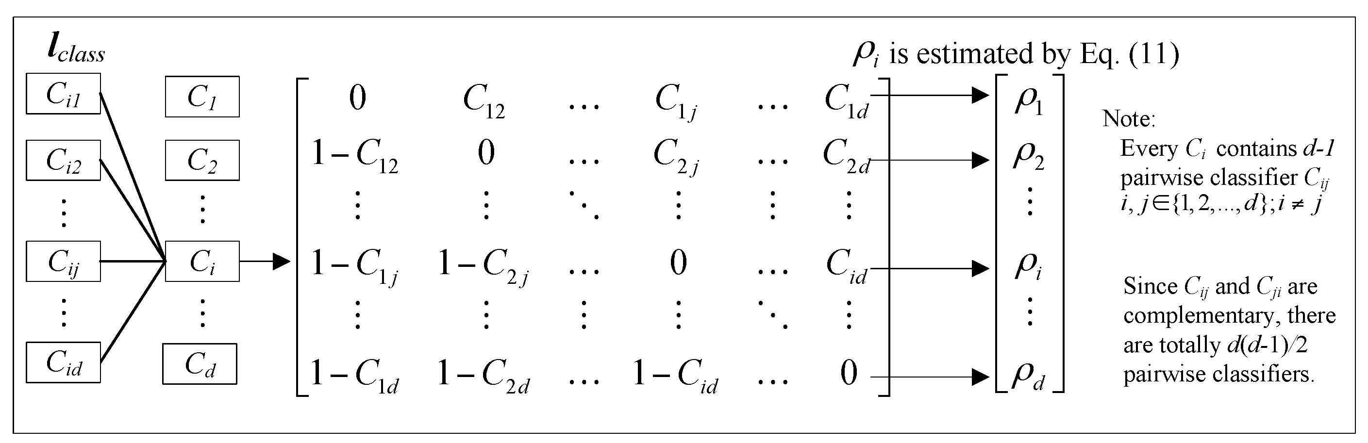
Figure 2. The pairwise coupling strategy also constructs a group of classifiers
lclass = [
C1,
C2, …,
Cd] in a
d-label classification problem. However, each
Ci = [
Ci1,
Ci2, …,
Cid] is composed of a set of
d − 1 different pairwise classifiers
Cij,
. Since
Cij and
Cji are complementary, there are totally
d(
d − 1)/2 classifiers in
lclass as shown in
Figure 3. To solve the multi-classification and probabilistic output problems, a pairwise coupling strategy is adopted for the RVM and PNN classifiers. The strategy combines all the outputs of every pair of classes to re-estimate the overall probability for a new instance.
Figure 2.
Indecisive regions (shaded regions) using one-vs-all (left) and pairwise coupling (right).
Figure 2.
Indecisive regions (shaded regions) using one-vs-all (left) and pairwise coupling (right).
Figure 3.
Pairwise coupling strategy of probabilistic classification.
Figure 3.
Pairwise coupling strategy of probabilistic classification.
There are several available methods for pairwise coupling strategy [
29], which are, however unsuitable for simultaneous-fault diagnosis because of the constraint
. Where
is the probability of the
ith label. Note that the nature of simultaneous-fault diagnosis is that
is unnecessarily equal to 1. Therefore, the following simple pairwise coupling strategy for simultaneous-fault diagnosis is proposed. Every
is calculated as:
where
nij is the number of training feature vectors with either the
ith or
jth label. Hence, the probability can be accurately estimated from
because the pairwise correlation between the labels is taken into account. With the above pairwise coupling strategy, the proposed probabilistic committee member, PCRVM, could estimate the probability vector
in a high level of accuracy.
After designing the pairwise coupling strategy for each probabilistic classifier, a new ensemble method is proposed to combine the result from each committee member with optimal weight.
2.2.3. Ensemble Method
One of the most frequently used ensemble methods is weighted averaging. In this method, every committee member has an appropriate weight related to its ability. However, the weighted averaging method cannot give a fair result when it deals with the issue of unbalanced committee member sensitivities to faults. For example, when the committee member 1 is not trained by a dataset with the fault
d5, the fault
d5 usually cannot be predicted by the committee member 1, which is demonstrated in
Table 2. However, the weight averaging method still uses the unpredictable output to calculate the overall average, resulting in an unfair or unpredictable result.
To overcome the above problem, a novel ensemble method with optimal weights and predefined null outputs is proposed which is given by Equation (12). In Equation (12),
is set to be zero when the
jth classifier cannot make a diagnosis for the
ith fault label (
i.e., the
jth classifier is not trained by the
ith single-fault). In this way, the proposed method can overcome the problem of the traditional weighted averaging method, which is one of main contributions of this research. The probability of the
ith fault is expressed as:
where
wj-opt is the optimal weight for the
jth committee member,
wj-opt ,
j = 1 to
k, where
k is the number of committee members, and the sum of
wj-opt is not equal to 1.
is probability estimated from the
jth classifier for the
ith single-fault,
i = 1 to
d where
d is the total number of detectable single-faults. Finally, the probabilistic outputs of classifiers are combined with optimal weights to generate the probability vector
P = [P
1, P
2, ...
, P
d].
Table 2.
Issue of weighted averaging method for balanced and unbalanced committee member sensitivities to gearbox faults.
Table 2.
Issue of weighted averaging method for balanced and unbalanced committee member sensitivities to gearbox faults.
| Balanced Member Sensitivities to Gearbox Faults | Committee Member 1 | Committee Member 2 | Average Output Probability (P3) for d3 |
|---|
| Fault d3 | trained | trained |
P3 is a reasonable result |
| Output probability for d3 for an unseen case | | |
| Unbalanced Member Sensitivities to Gearbox Faults | Committee Member 1 | Committee Member 2 | Average Output Probability (P5) for d5 |
| Fault d5 | Unable to train | trained |
P5 is an unfair/unpredictable result |
| Output probability for d5 for an unseen case | is unpredictable | |
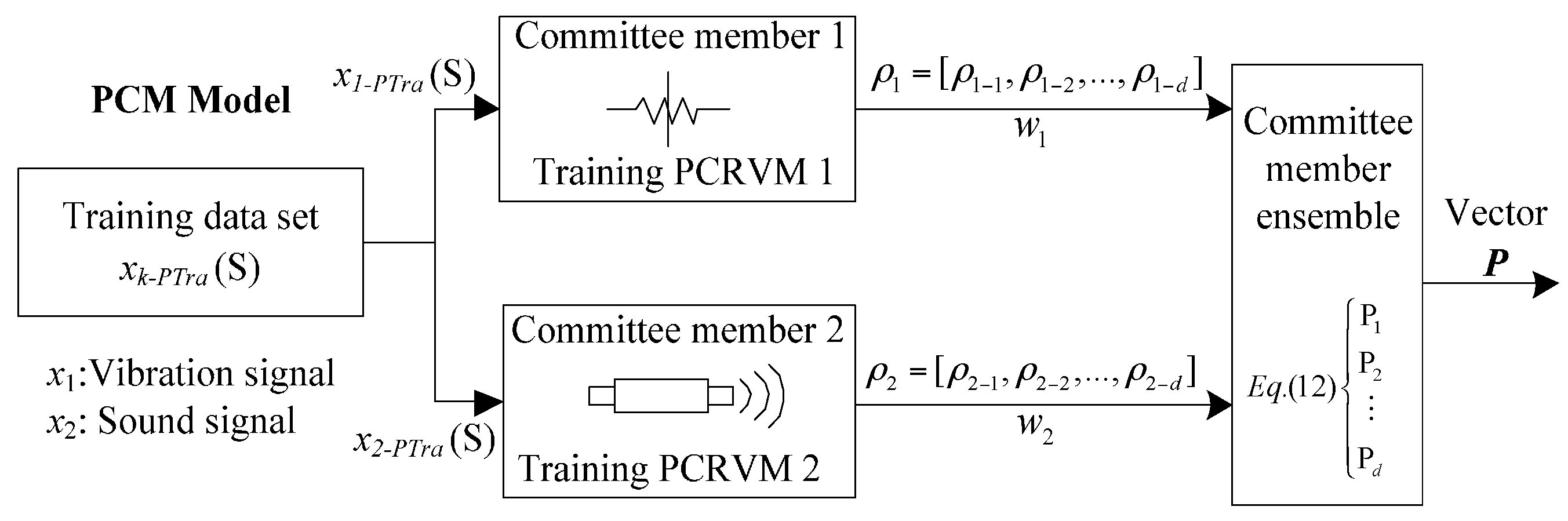
In this application, the processed training datasets
xk-PTra, are employed to train probabilistic classifiers (PCRVM) respectively. The workflow of the PCM is shown in
Figure 4.
Figure 4.
Procedure for training probabilistic committee machine.
Figure 4.
Procedure for training probabilistic committee machine.
2.3. Parameter Optimization
The probability vector
P = [P
1, P
2, …, P
d] can be provided to the user as a quantitative measure for reference and further processing. However, human experts generally cannot identify the number of simultaneous-faults directly based on the output probability of each fault. Therefore, a decision threshold (DT)
ε is introduced to identify the simultaneous-faults from
P such that:
where
and
denotes that the corresponding fault occurs. For example, given an unseen input
x, if
P = [0.72, 0.42, 0.51, 0.81, 0.39] and
ε = 0.5, then
y = DT(
P) = [1, 0, 1, 1, 0]. Therefore, the unseen
x is diagnosed as a simultaneous-fault for the labels (1, 3, 4).
Obviously, the weight and the decision threshold are the major factors affecting the classification accuracy. By reviewing the literature [
30,
31], it is seen that PSO has the same effectiveness as a typical optimization method, genetic algorithms, in finding the global optimal solution, but with better computational efficiency. Hence, PSO is adopted to determine the best weights
wopt and decision threshold
εopt in this study.
Particle Swarm Optimization
PSO is a population-based optimizer. The population is regarded as a swarm and the individuals are considered as particles. For an
z-dimensional search space and a swarm consisting of
H particles, the
ith particle can be represented by an
z-dimensional vector
ui = (
ui1,
ui2, …,
uiz), the velocity of this particle can be an
z-dimensional vector
vi = (
vi1,
vi2, …,
viz), and the best previous position encountered by this particle can be described as
pi = (
pi1,
pi2, …,
piz). Let
g represent the index of the particle that attains the best previous position among all the particles in the swarm. Then, the swarm is manipulated in accordance with the following equations:
where
i is the particle index
i = [1, 2, …,
H],
Wf is the weight factor,
q1 and
q2 are positive constants,
r1 and
r2 are the random numbers selected between [0, 1]. The selection of the above parameters was presented in [
36]. With reference to the literature,
Table 3 shows the PSO parameters selected for this case study.
Table 3.
PSO parameters.
| Number of generations | 1000 |
| Population size | 50 |
| Wf | 0.9 |
| q1 | 2 |
| q2 | 2 |
To evaluate the fitness of each iteration, a common evaluation method called
F-measure [
37] and an objective function described in
Section 2.4 are employed. The procedure of the proposed PSO approach is illustrated in
Figure 5, which is performed in three steps:
- (1)
Initializing the parameters of PSO: The candidate weight (w1, w2) and decision threshold are randomly selected from interval [0, 1].
- (2)
Calculating the output of
F-measure: Following the procedure in
Figure 5, the candidate weight and decision threshold are entered into the PCM model and Equation (13), respectively.
- (3)
Comparing the output of F-measure with the objective function: If the F-measure satisfies the objective function, the corresponding weights and decision threshold are taken as optimal parameters, otherwise PSO updates the weights and decision threshold based on Equations (14) and (15), and then repeats Steps 2 and 3. When it reaches the present number of generation or satisfies the objective function, the corresponding weights and decision threshold of the highest output of F-measure are taken as optimal parameters.
Figure 5.
Procedure for optimization of committee member weights and decision threshold.
Figure 5.
Procedure for optimization of committee member weights and decision threshold.
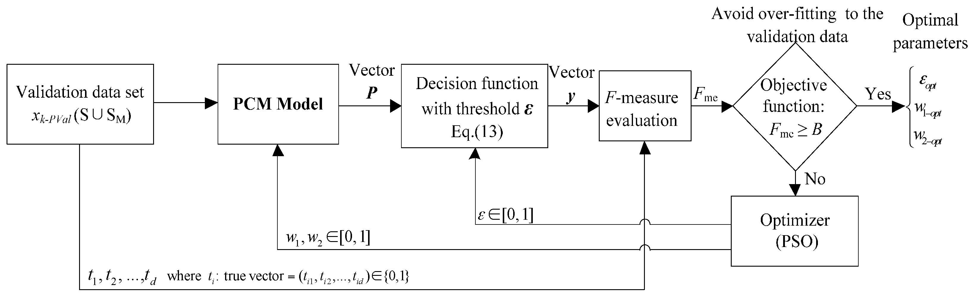
2.4. Performance Evaluation
The traditional performance evaluation of classifiers only considers exact matching of the decision vector
y against the true vector
t. This evaluation is however unsuitable for simultaneous-fault diagnosis where partial matching is preferred.
F-measure is mostly used as a performance evaluation for information retrieval systems where a document may belong to a single or multiple tags simultaneously, which is very similar to the current study. By using
F-measure, the evaluation of both single-fault and simultaneous-fault test cases can be fairly examined. The definition of
F-measure is given in Equation (16). The larger the
F-measure value, the higher the diagnostic accuracy is:
where
yi = [
yi1,
yi2, …,
yid] and
ti = [
ti1,
ti2, …,
tid] are the predicted decision vector and the true decision vector respectively, for
j = 1 to
d and
i = 1 to
Nt and ∀
yij,
tij ∈ [0, 1].
Nt is the number of single-fault and simultaneous-fault test patterns. For optimization of the weights and decision threshold,
Fme also serves as an important parameter in an objective function. In order to avoid over-fitting to the validation dataset and achieve high diagnostic accuracy, the objective function is specifically defined as:
where
B is the preset optimal accuracy of
F-measure and
B lies between 0 and 1. In this study,
B is set to be 0.9 as a trial.
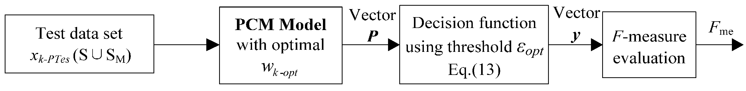
Figure 6 summarizes the evaluation process for the proposed diagnostic framework.
Figure 6.
Evaluation of proposed framework.
Figure 6.
Evaluation of proposed framework.
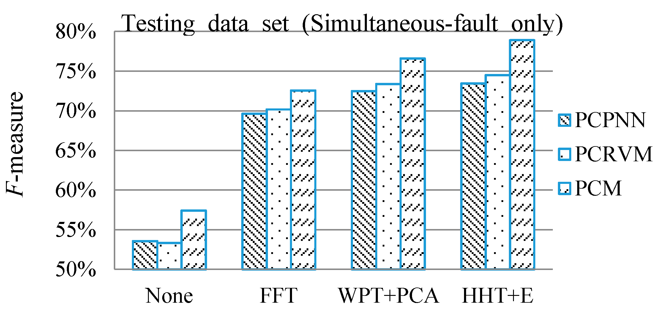
5. Conclusions
In this paper, a new framework, which combines signal de-noising, feature extraction, probabilistic committee machine, parameter optimization and F-measure, has successfully been developed to overcome the challenges of simultaneous fault diagnosis and multiple signal analysis in a gearbox. In consideration of the features of vibration and sound signals in this application, DWT and HHT + E are used for signal de-noising and feature extraction, respectively, so that the diagnostic system can effectively capture the single fault components from the noise-polluted simultaneous fault patterns. It implies that the acquisition of large amount of simultaneous fault signals can be avoided. Moreover, PSO is effective for optimizing the weight of each committee member and decision threshold in the PCM framework. To verify the effectiveness of the proposed probabilistic committee machine and make a comparison, the single probabilistic classifiers, PCPNN and PCRVM, are also employed to diagnose the simultaneous faults. Although the results show that those machine learning methods can diagnose the simultaneous faults in the gearbox, it is found that the proposed PCM framework is superior to the single classifiers. Therefore, the proposed PCM framework is suitable to detect the simultaneous faults in the gearbox.
In practice, most mechanical faults can be diagnosed by analyzing vibrations, sounds, currents, oil debris and temperature signals. As the number and type of committee members in the proposed framework can be adjusted by the user, the proposed framework can be applied to other similar diagnostic applications.


