
ReliefF-Based EEG Sensor Selection Methods for Emotion Recognition


Abstract
:1. Introduction
2. Materials and Methods
2.1. DEAP Database
2.2. Feature Extraction
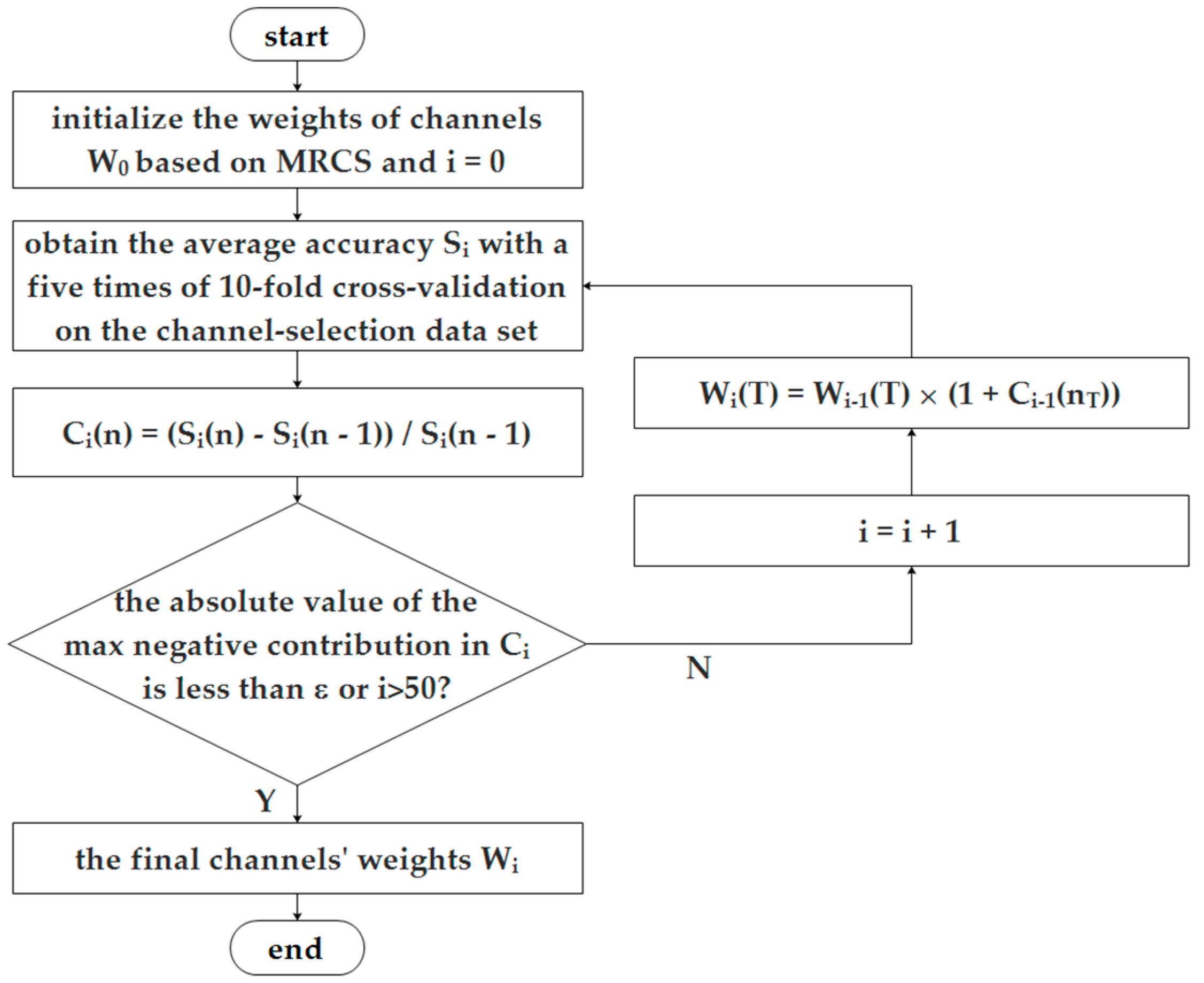
2.3. Channel Selection Based on ReliefF
- set all the weights of 128 features to zero, ;
- for i = 1 to the number of samples in the channel-selection dataset do
- select a sample Ri;
- find k nearest hits ;
- for each class C ≠ class(Ri) do
- find k nearest misses Mj(C)(j = 1, 2, …, k) from class C;
- end;
- for l = 1 to 128 do
- end;
- end;
2.4. Classifiers to Evaluate the Performance
3. Results
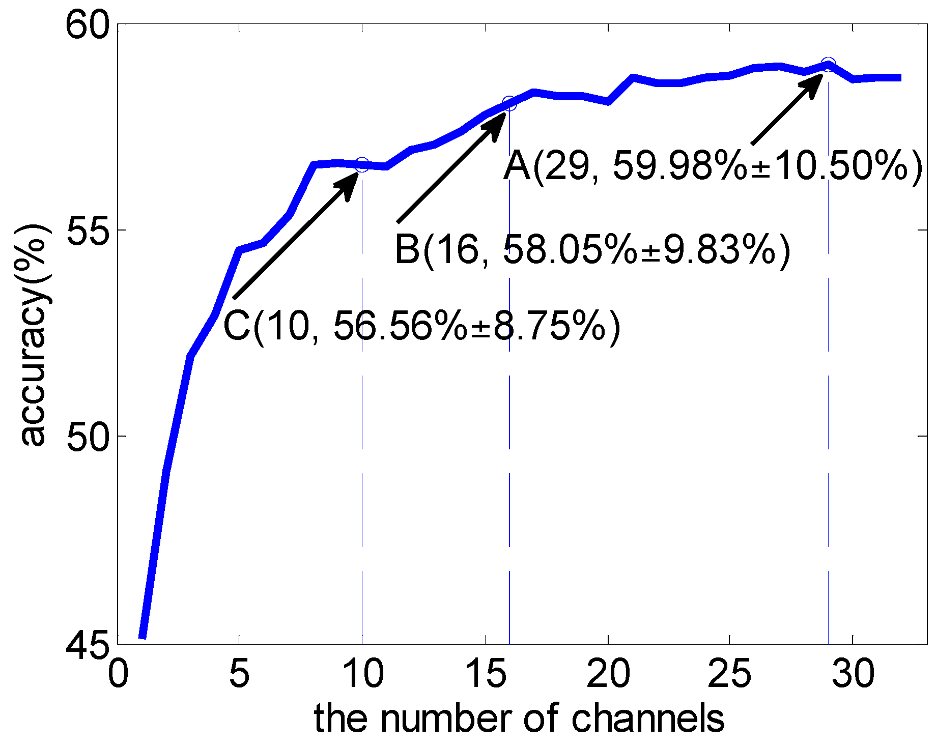
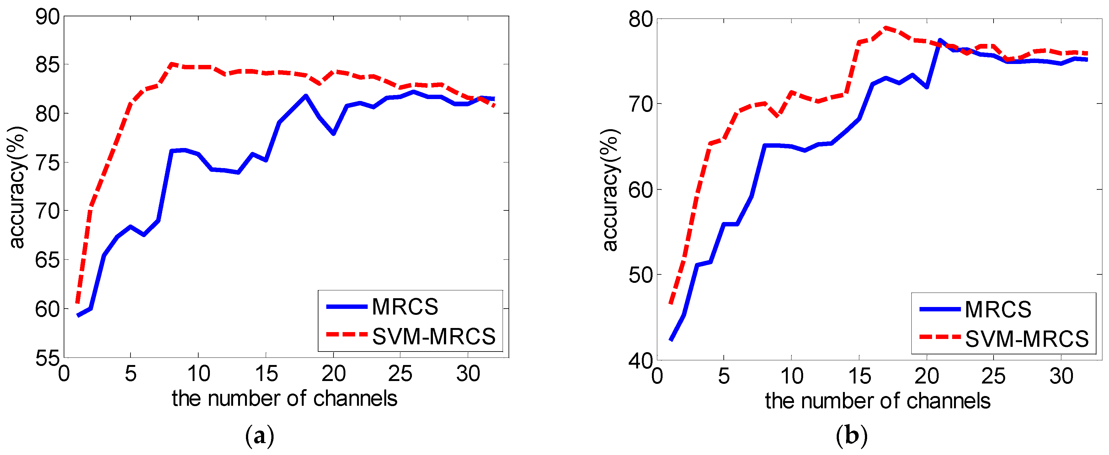
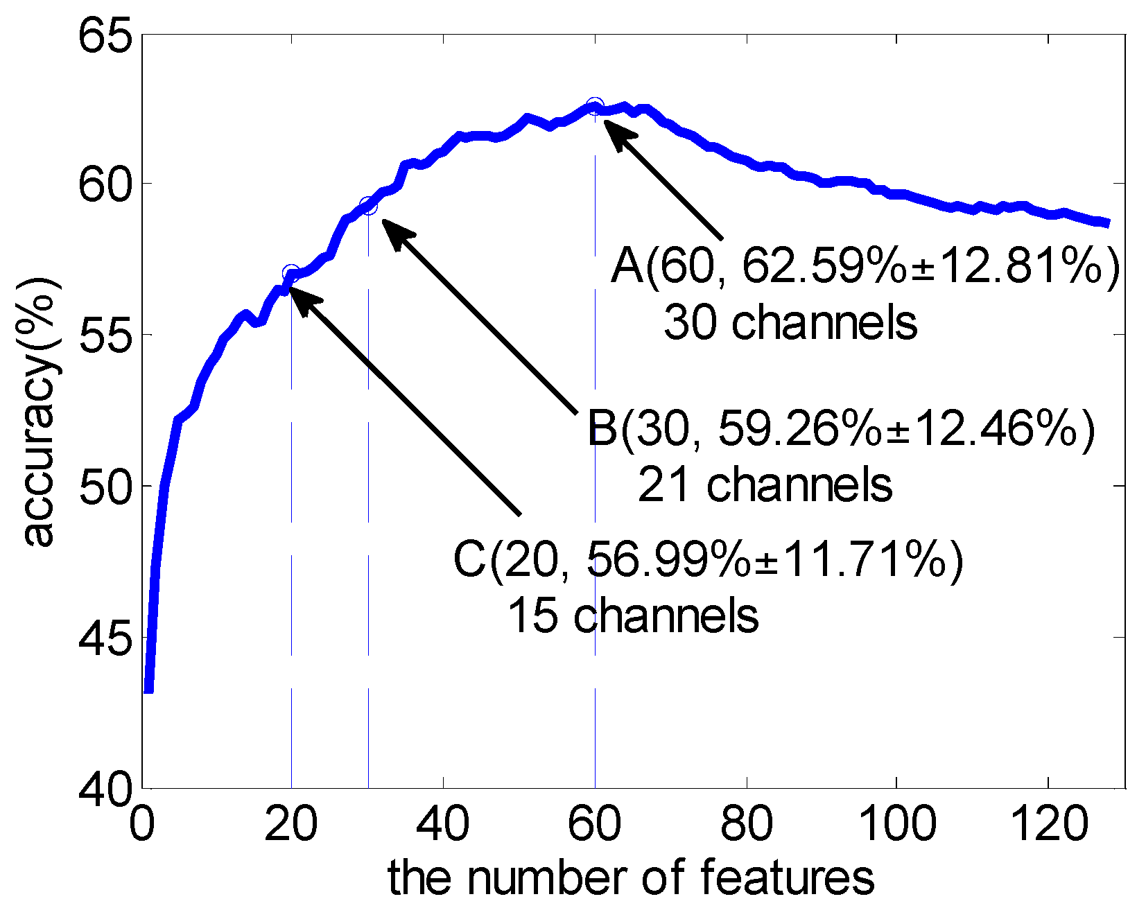
3.1. Subject-Dependent Channel Selection
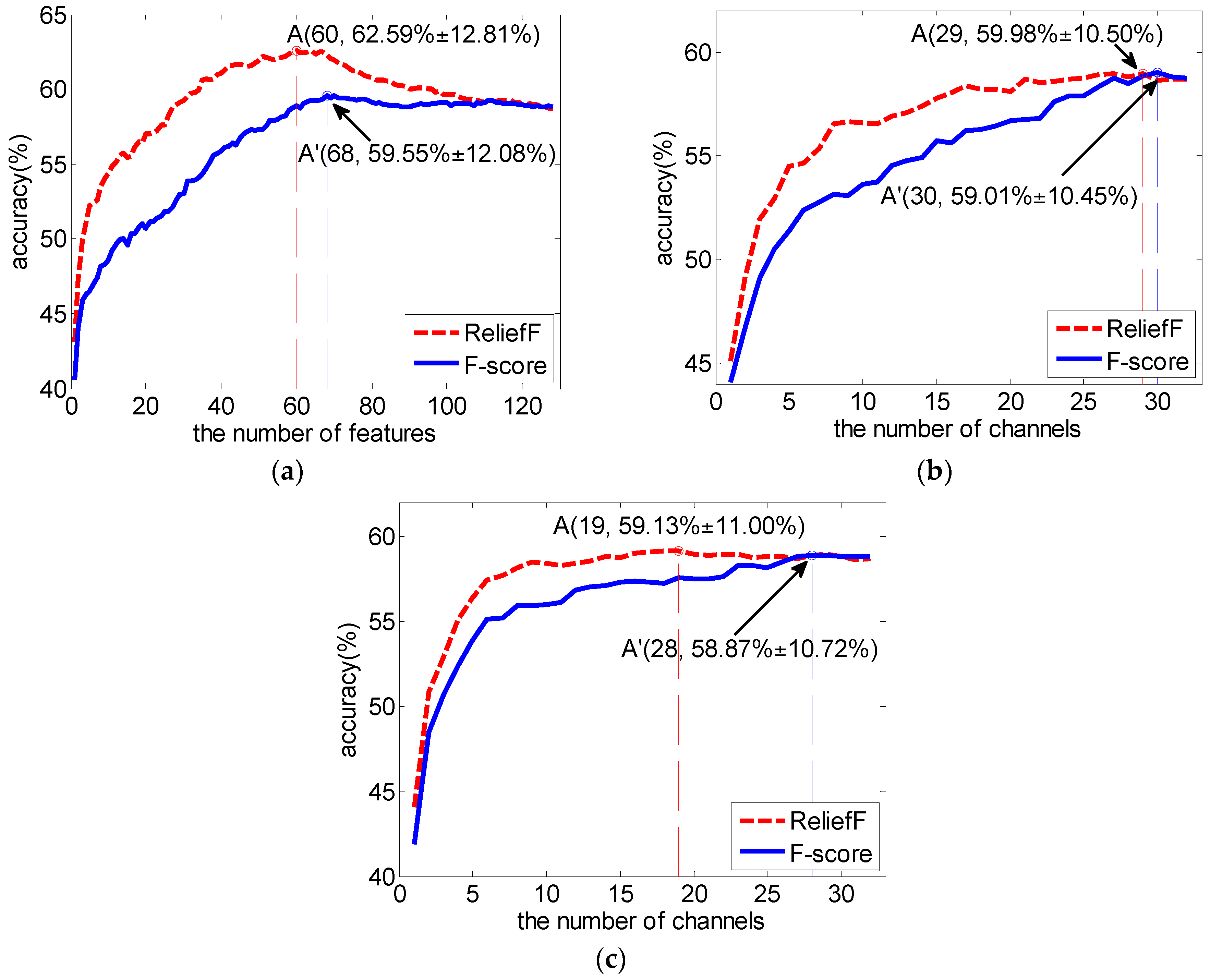
3.2. Comparison with F-Score as Feature Selection Method
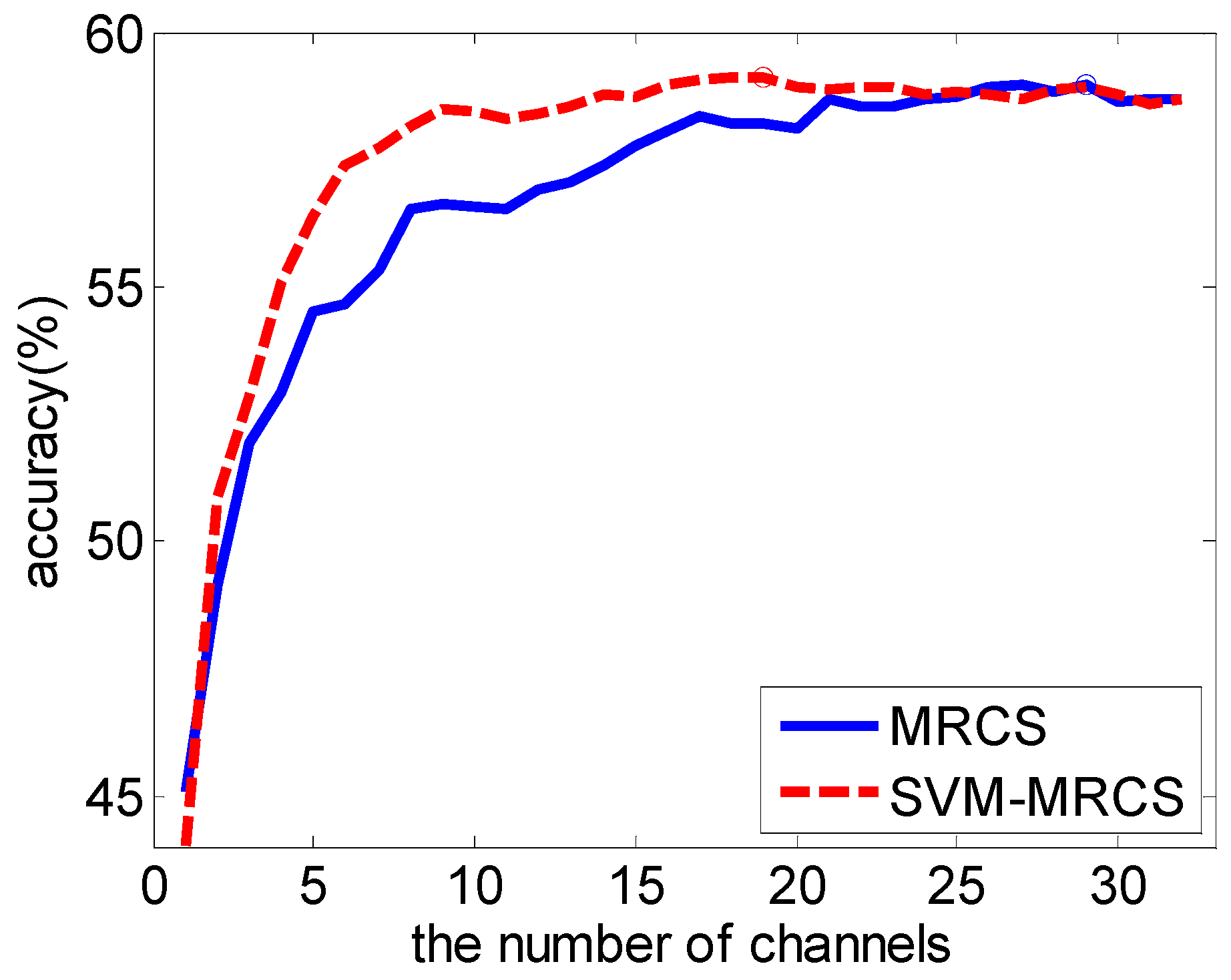
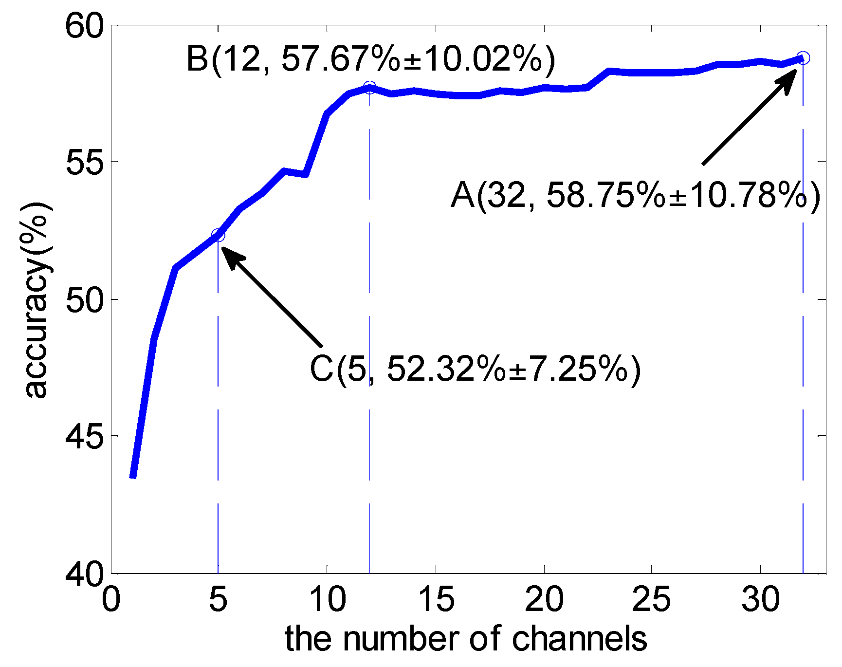
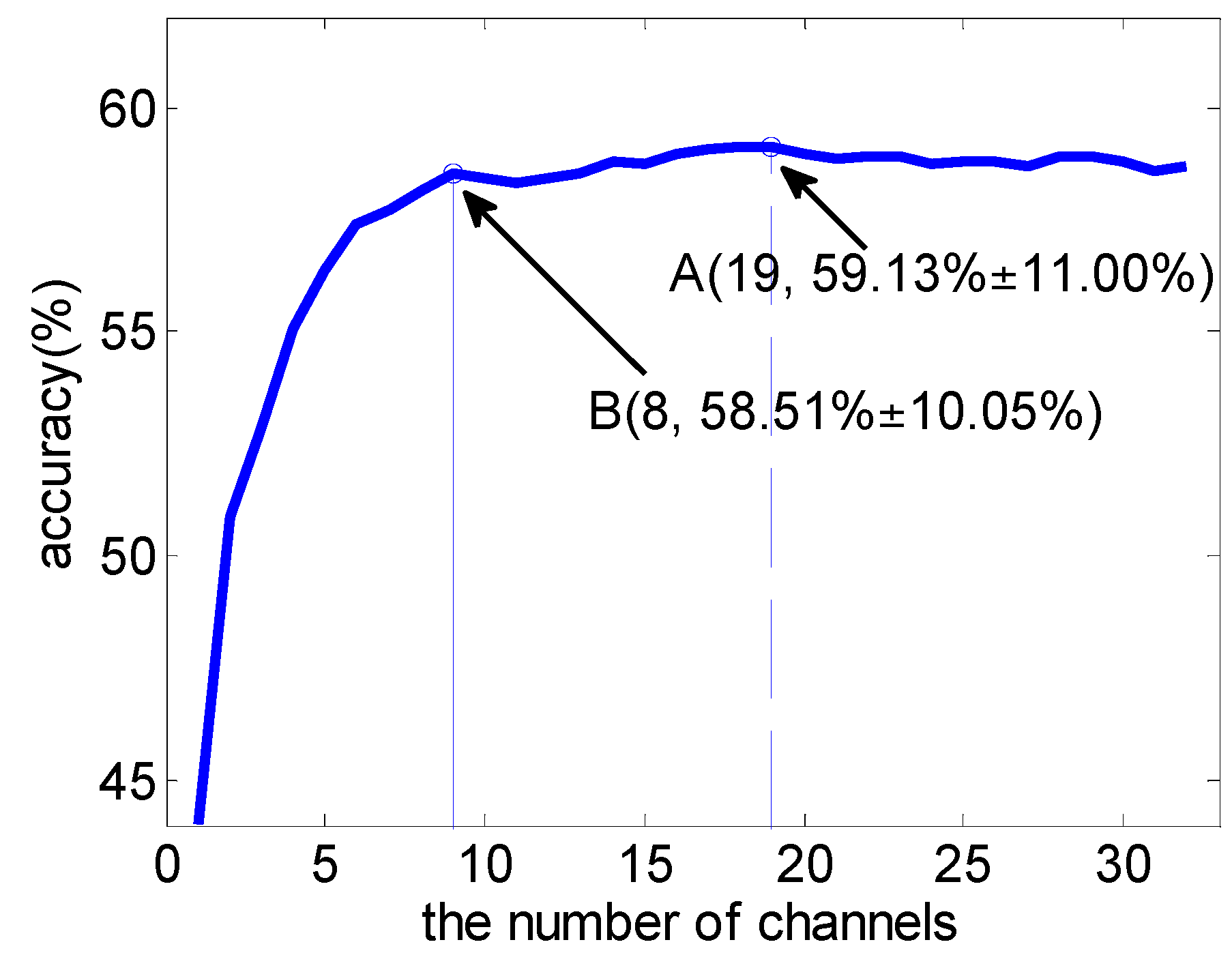
3.3. Subject-Independent Channel Selection
4. Discussion
5. Conclusions
Acknowledgments
Author Contributions
Conflicts of Interest
References
- Picard, R.W. Affective computing. IGI Glob. 1995, 1, 71–73. [Google Scholar]
- Petrushin, V.A. Emotion in Speech: Recognition and Application to Call Centers. Available online: http://citeseer.ist.psu.edu/viewdoc/download?doi=10.1.1.42.3157&rep=rep1&type=pdf (accessed on 18 September 2016).
- Picard, R.W.; Vyzas, E.; Healey, J. Toward machine emotional intelligence: Analysis of affective physiological state. IEEE Trans. Pattern Anal. Mach. Intell. 2001, 23, 1175–1191. [Google Scholar] [CrossRef]
- Anderson, K.; McOwan, P.W. A real-time automated system for the recognition of human facial expressions. IEEE Trans. Syst. Man Cybern. Part B Cybern. A Publ. IEEE Syst. Man Cybern. Soc. 2006, 36, 96–105. [Google Scholar] [CrossRef]
- Lal, T.N.; Schröder, M.; Hinterberger, T.; Weston, J.; Bogdan, M.; Birbaumer, N.; Schölkopf, B. Support vector channel selection in bci. IEEE Trans. Biomed. Eng. 2004, 51, 1003–1010. [Google Scholar] [CrossRef] [PubMed]
- Sannelli, C.; Dickhaus, T.; Halder, S.; Hammer, E.M.; Müller, K.R.; Blankertz, B. On optimal channel configurations for smr-based brain-computer interfaces. Brain Topogr. 2010, 23, 186–193. [Google Scholar] [CrossRef] [PubMed]
- Arvaneh, M.; Guan, C.; Ang, K.K.; Quek, C. Optimizing the channel selection and classification accuracy in EEG-based bci. Biomed. Eng. IEEE Trans. 2011, 58, 1865–1873. [Google Scholar] [CrossRef] [PubMed]
- Bos, D.O. EEG-based emotion recognition The Influence of Visual and Auditory Stimuli. Emotion 2006, 1359, 667–670. [Google Scholar]
- Zhang, Q.; Lee, M. Letters: Analysis of positive and negative emotions in natural scene using brain activity and gist. Neurocomputing 2009, 72, 1302–1306. [Google Scholar] [CrossRef]
- Schmidt, L.A.; Trainor, L.J. Frontal brain electrical activity (EEG) distinguishes valence and intensity of musical emotions. Cogn. Emot. 2001, 15, 487–500. [Google Scholar] [CrossRef]
- Valenzi, S.; Islam, T.; Jurica, P.; Cichocki, A. Individual classification of emotions using EEG. J. Biomed. Sci. Eng. 2014, 7, 604–620. [Google Scholar] [CrossRef]
- Lin, Y.P.; Wang, C.H.; Jung, T.P.; Wu, T.L.; Jeng, S.K.; Duann, J.R.; Chen, J.H. EEG-based emotion recognition in music listening. IEEE Trans. Biomed. Eng. 2010, 57, 1798–1806. [Google Scholar] [PubMed]
- Hamann, S. Mapping discrete and dimensional emotions onto the brain: Controversies and consensus. Trends Cogn. Sci. 2012, 16, 458–466. [Google Scholar] [CrossRef] [PubMed]
- Alotaiby, T.; El-Samie, F.E.A.; Alshebeili, S.A.; Ahmad, I. A review of channel selection algorithms for EEG signal processing. EURASIP J. Adv. Signal Process. 2015, 2015, B172. [Google Scholar] [CrossRef]
- Wang, X.-W.; Nie, D.; Lu, B.-L. EEG-Based Emotion Recognition Using Frequency Domain Features and Support Vector Machines. In Proceedings of the International Conference on Neural Information Processing (ICONIP 2011), Shanghai, China, 13–17 November 2011; pp. 734–743.
- Jatupaiboon, N.; Pan-Ngum, S.; Israsena, P. Emotion classification using minimal EEG channels and frequency bands. In Proceedings of the International Joint Conference on Computer Science and Software Engineering, Khon Kaen, Thailand, 29–31 May 2013; pp. 21–24.
- Robnik-Šikonja, M.; Kononenko, I. Theoretical and empirical analysis of relieff and rrelieff. Mach. Learn. 2003, 53, 23–69. [Google Scholar] [CrossRef]
- Koelstra, S.; Muhl, C.; Soleymani, M.; Lee, J.S.; Yazdani, A.; Ebrahimi, T.; Pun, T.; Nijholt, A.; Patras, I. Deap: A database for emotion analysis using physiological signals. IEEE Trans. Affect. Comput. 2011, 3, 18–31. [Google Scholar] [CrossRef]
- Russell, J.A. A circumplex model of affect. J. Pers. Soc. Psychol. 1980, 39, 1161–1178. [Google Scholar] [CrossRef]
- Frydenlund, A.; Rudzicz, F. Emotional affect estimation using video and EEG data in deep neural networks. Lect. Notes Comput. Sci. 2015, 9091, 273–280. [Google Scholar]
- Pham, T.; Ma, W.; Tran, D.; Tran, D.S. A Study on the Stability of EEG Signals for User Authentication. In Proceedings of the International IEEE/EMBS Conference on Neural Engineering, Montpellier, France, 22–24 April 2015; pp. 122–125.
- Liu, Y.; Sourina, O. Real-Time Subject-Dependent EEG-Based Emotion Recognition Algorithm; Springer: Heidelberg, Germany, 2014; pp. 199–223. [Google Scholar]
- Candra, H.; Yuwono, M.; Chai, R.; Handojoseno, A.; Elamvazuthi, I.; Nguyen, H.T.; Su, S. Investigation of window size in classification of EEG-emotion signal with wavelet entropy and support vector machine. In Proceedings of the International Conference of the IEEE Engineering in Medicine and Biology Society, Milan, Italy, 25–29 August 2015; pp. 7250–7253.
- Jenke, R.; Peer, A.; Buss, M. Feature extraction and selection for emotion recognition from EEG. IEEE Trans. Affect. Comput. 2014, 5, 327–339. [Google Scholar] [CrossRef]
- Schaaff, K.; Schultz, T. Towards emotion recognition from electroencephalographic signals. In Proceedings of the Affective Computing and Intelligent Interaction and Workshops, Amsterdam, The Netherlands, 10–12 September 2009; pp. 1–6.
- Chang, C.C.; Lin, C.J. LIBSVM: A library for support vector machines. ACM Trans. Intell. Syst. Technol. 2011, 2, 1–27. [Google Scholar] [CrossRef]
- Zheng, W.L.; Lu, B.L. Investigating critical frequency bands and channels for EEG-based emotion recognition with deep neural networks. IEEE Trans. Auton. Ment. Dev. 2015, 7, 162–175. [Google Scholar] [CrossRef]


| Top-N Features | Average Number of Channels Involved | Average Accuracy (%) |
|---|---|---|
| 4 | 3.25 (0.77) | 51.04 (8.32) |
| 8 | 6.56 (1.36) | 53.47 (11.21) |
| 12 | 9.44 (2.06) | 55.13 (10.77) |
| 16 | 12.13 (2.58) | 55.49 (11.31) |
| 20 | 14.88 (2.99) | 56.99 (11.71) |
| 24 | 17.50 (3.39) | 57.58 (12.14) |
| 28 | 19.50 (3.65) | 58.93 (12.83) |
| 32 | 21.44 (4.21) | 59.70 (12.38) |
| 36 | 23.25 (4.09) | 60.69 (12.74) |
| 40 | 24.50 (3.72) | 61.09 (12.54) |
| 50 | 27.25 (2.96) | 61.86 (12.80) |
| 60 | 29.63 (2.60) | 62.59 (12.81) |
| 80 | 31.13 (1.15) | 60.76 (11.54) |
| Top-N Features | The Average Proportion of Each Class of Features | |||
|---|---|---|---|---|
| Theta | Alpha | Beta | Gamma | |
| 4 | 0.03 | 0.02 | 0.27 | 0.68 |
| 8 | 0.04 | 0.09 | 0.18 | 0.69 |
| 16 | 0.07 | 0.11 | 0.25 | 0.57 |
| 32 | 0.10 | 0.12 | 0.29 | 0.49 |
| 64 | 0.13 | 0.13 | 0.35 | 0.39 |
| 96 | 0.20 | 0.21 | 0.29 | 0.30 |
| 128 | 0.25 | 0.25 | 0.25 | 0.25 |
| Average Accuracy (Standard Deviation) Using Top-N Channels | |||||
|---|---|---|---|---|---|
| Top-N | MRCS | SVM-MRCS | Top-N | MRCS | SVM-MRCS |
| 3 | 51.95 (8.23) | 52.86 (8.41) | 12 | 56.93 (8.95) | 58.40 (10.20) * |
| 4 | 52.94 (7.49) | 55.08 (8.98) | 13 | 57.06 (9.01) | 58.54 (10.08) * |
| 5 | 54.51 (8.30) | 56.39 (8.95) | 14 | 57.38 (9.38) | 58.78 (10.27) * |
| 6 | 54.66 (8.89) | 57.39 (9.52) ** | 15 | 57.79 (9.34) | 58.73 (10.40) |
| 7 | 55.34 (8.90) | 57.71 (9.53) ** | 16 | 58.05 (9.83) | 58.97 (10.75) |
| 8 | 56.55 (8.92) | 58.16 (9.47) * | 17 | 58.34 (9.63) | 59.08 (10.92) |
| 9 | 56.62 (8.98) | 58.51 (10.05) * | 18 | 58.21 (9.61) | 59.10 (11.05) |
| 10 | 56.56 (8.75) | 58.43 (9.90) * | 19 | 58.22 (9.80) | 59.13 (11.00) |
| 11 | 56.53 (8.72) | 58.31 (10.05) * | 20 | 58.09 (9.79) | 58.93 (10.95) |
| Channel Rank | Electrode | Brain Lobe |
|---|---|---|
| 1 | Fp1 | Frontal |
| 2 | T7 | Temporal |
| 3 | PO4 | Parietal |
| 4 | Pz | Parietal |
| 5 | Fp2 | Frontal |
| 6 | F8 | Frontal |
| 7 | Oz | Occipital |
| 8 | T8 | Temporal |
| 9 | P4 | Parietal |
| 10 | O1 | Occipital |
| 11 | AF4 | Frontal |
| 12 | FC5 | Frontal |
| 13 | C3 | Central |
| 14 | FC2 | Frontal |
| 15 | P3 | Parietal |
© 2016 by the authors; licensee MDPI, Basel, Switzerland. This article is an open access article distributed under the terms and conditions of the Creative Commons Attribution (CC-BY) license (http://creativecommons.org/licenses/by/4.0/).
Share and Cite
Zhang, J.; Chen, M.; Zhao, S.; Hu, S.; Shi, Z.; Cao, Y. ReliefF-Based EEG Sensor Selection Methods for Emotion Recognition. Sensors 2016, 16, 1558. https://doi.org/10.3390/s16101558
Zhang J, Chen M, Zhao S, Hu S, Shi Z, Cao Y. ReliefF-Based EEG Sensor Selection Methods for Emotion Recognition. Sensors. 2016; 16(10):1558. https://doi.org/10.3390/s16101558
Chicago/Turabian StyleZhang, Jianhai, Ming Chen, Shaokai Zhao, Sanqing Hu, Zhiguo Shi, and Yu Cao. 2016. "ReliefF-Based EEG Sensor Selection Methods for Emotion Recognition" Sensors 16, no. 10: 1558. https://doi.org/10.3390/s16101558
APA StyleZhang, J., Chen, M., Zhao, S., Hu, S., Shi, Z., & Cao, Y. (2016). ReliefF-Based EEG Sensor Selection Methods for Emotion Recognition. Sensors, 16(10), 1558. https://doi.org/10.3390/s16101558