Passive Localization of Mixed Far-Field and Near-Field Sources without Estimating the Number of Sources

Abstract

This paper presents a novel algorithm for the localization of mixed far-field sources (FFSs) and near-field sources (NFSs) without estimating the source number. Firstly, the algorithm decouples the direction-of-arrival (DOA) estimation from the range estimation by exploiting fourth-order spatial-temporal cumulants of the observed data. Based on the joint diagonalization structure of multiple spatial-temporal cumulant matrices, a new one-dimensional (1-D) spatial spectrum function is derived to generate the DOA estimates of both FFSs and NFSs. Then, the FFSs and NFSs are identified and the range parameters of NFSs are determined via beamforming technique. Compared with traditional mixed sources localization algorithms, the proposed algorithm avoids the performance deterioration induced by erroneous source number estimation. Furthermore, it has a higher resolution capability and improves the estimation accuracy. Computer simulations are implemented to verify the effectiveness of the proposed algorithm.

1. Introduction

Source localization has received considerable attention in sensor array signal processing over the past decades [1]. Most of the existing algorithms concentrate on far-field sources (FFSs), whose wavefronts are plane waves. Many high resolution algorithms have been proposed for the direction-of-arrival (DOA) estimation under the far-field assumption, such as the multiple signal classification (MUSIC) method [2], the estimation of signal parameters via rotational invariance technique (ESPRIT) [3], and their derivatives [4–6]. However, in many practical applications, the radiating sources may lie in the Fresnel region of the array [7], which is defined as [0.62(D²/λ)^½, 2D²/λ] where λ is the wavelength of the sources and D symbolizes the array aperture. In this region, the spherical wavefronts are characterized by both DOA and range parameters [8]. Consequently, traditional FFS DOA estimation algorithms are no longer applicable for near-field sources (NFSs) localization. Fortunately, many advanced algorithms have been proposed for NFSs localization, including the 2-D MUSIC algorithm [8], the covariance approximation (CA) method [9,10], the weighted linear prediction method [11], and the rank-reduction (RARE) type algorithms [12–14].

Moreover, both FFSs and NFSs may coexist in many situations of interest, such as seismic exploration, electronic surveillance and speaker localization using microphone arrays. Most of the algorithms which deal with pure FFSs or pure NFSs, may fail in the scenarios of mixed sources. Accordingly, there has been an increasing interest in mixed sources localization. A two-stage MUSIC (TSMUSIC) algorithm [15] is firstly developed to localize mixed FFSs and NFSs. Based on fourth order cumulants, the TSMUSIC algorithm can successfully estimate the parameters of mixed sources. However, its computational complexity is high due to the construction of high order cumulant matrices. To relieve the computational burden, an efficient oblique projection MUSIC (OPMUSIC) algorithm is proposed in [16], which only utilizes second-order statistics. However, this algorithm suffers from severe array aperture loss. In [17], a low-complexity ESPRIT algorithm is advanced to locate the mixed far-field and near-field cyclostationary sources. Yet, array aperture loss and reduced range estimation accuracy are two slight limitations of this method. In [18], the authors extend the array aperture by utilizing a special nested sparse linear array, which can improve the estimation accuracy. Unfortunately, the range estimation suffers from spurious peaks problem in this scheme. Based on the generalized ESPRIT (GESPRIT) algorithm [19], many algorithms have been proposed to localize mixed sources [20–23]. In [22], the related far-field components are eliminated from the signal subspace to improve the estimation accuracy. But its far-field component elimination technique would bring extra estimation errors. A covariance differencing method is proposed in [20,21] to generate more reasonable classification of the source types. Based on ESPRIT-Like and polynomial rooting, an efficient mixed sources localization algorithm is presented in [23]. However, for these GESPRIT-based algorithms, the number of NFSs they can resolve is less than half of the number of array sensors [24]. In [25–27], the authors utilize the sparse signal recovery technique for mixed sources localization, which provide improved estimation accuracy. The algorithms in [26,27] are based on the construction of fourth order cumulant matrices and vectors, whereas the anti-diagonal elements of the second-order array covariance matrix is exploited in [25]. However, these sparse-recovery-based algorithms call for an enormous amount of computations. Besides, the regularization parameter that balances the tradeoff between Frobenius norm and ℓ₁ norm is difficult to determine.

Note that all of the previous algorithms are based on linear array configurations which assume that the array sensors are placed along the y-axis and the sources are located in the y-z plane. Therefore, only two-dimensional (2-D) parameters (elevation angles and ranges) need to be estimated. Recently, some methods are developed to localize mixed sources in the three-dimensional (3-D) space, which is characterized by range, azimuth angle and elevation angle. For these algorithms, the geometric structure of the array is critical for the localization performance. Based on a cross array, the authors in [28] have decoupled the 3-D parameters estimation problem into one-dimensional (1-D) spectral functions in three stages. Also, a separated steering vector-based algorithm is proposed in [29] using cross array configuration. In [30], spherical microphone arrays are utilized for 3-D localization. By exploiting the recurrent relation between spherical harmonics, the DOAs are obtained from ESPRIT-like approach and the ranges are determined by 1-D MUSIC spectral search.

However, all of the abovementioned methods are based on subspace decomposition, which requires exact determination of the source number. Although some designed criteria, such as the Akaike information criterion (AIC) [31] and the minimum description length (MDL) detection criterion [32], can be used to estimate the source number, they tend to generate erroneous estimates of the number of sources under the condition of low signal-to-noise ratio (SNR) and small sample size [33]. Furthermore, most of these methods need that both the number of FFSs and the number of NFSs are known or correctly estimated, which is an even more difficult task in practical applications. If the source enumeration of the FFSs or the NFSs is incorrect, these subspace based methods will suffer from performance deterioration induced by underestimation as well as overestimation of the subspace dimension.

In view of the previous analyses, the mixed sources localization problem is faced with the following main difficulties: (1) being able to localize mixed sources successfully with unknown source number; (2) reasonable classification of FFSs and NFSs; (3) avoiding multidimensional search; (4) alleviating aperture loss; (5) avoiding parameter matching.

Aiming at addressing the abovementioned difficulties, we propose in this paper a novel localization algorithm for mixed FFSs and NFSs. Firstly, we construct multiple fourth-order spatial-temporal cumulant matrices, which only depend on the DOA information. Based on the joint diagonalization structure of these matrices, a novel 1-D spatial spectrum function is derived to generate the DOA estimates of both FFSs and NFSs. Then, with the DOA estimates, the range parameters are obtained and automatically paired via beamforming technique. Also, the types the sources are reasonably identified. Compared with the traditional methods, the proposed one does not require the knowledge of the source number, and therefore prevents the performance deterioration induced by erroneous source enumeration. In addition, our method avoids multidimensional spectral search and aperture loss. Moreover, both the temporal and spatial structures of the observed data are utilized in our method, which also contribute to the improvement of resolution ability and estimation accuracy. Due to the linear array configuration, our algorithm is limited to localize mixed sources only in the 2-D domain (elevation angle and range). To address the azimuth-elevation-range (3-D) localization problem, we can extend the proposed algorithm by applying planar arrays, such as cross array, rectangular array and circular array.

The rest of the paper is organized as follows: Section 2 introduces the signal model of mixed FFSs and NFSs. The proposed method is described in Section 3. In Section 4, we reveal a relationship between TSMUSIC and the proposed method. Section 5 presents a comparison among TSMUIC, OPMUSIC and the proposed algorithm. In Section 6, simulations are conducted to validate the performance of our method. We conclude this paper in Section 7.

Throughout the paper, the complex conjugate, transpose, Hermitian transpose, pseudo inverse are denoted by (•)*, (•)^T, (•)^H and (•)^†, respectively. I_m represents a m × m identity matrix, and 0_m,n is a m × n zero matrix.

2. Problem Formulation

Consider K independent narrowband sources (near-field or far-field) sensed by a symmetric uniform linear sensor array (ULSA), which is composed of 2M + 1 omnidirectional sensors, as shown in Figure 1. All of these sensors are placed along the y-axis, with the inter-element spacing being d. Moreover, we assume that the impinging signals are in the y-z plane. As shown in Figure 1, the azimuth angles of impinging sources become 90° in this scenario, therefore, only the elevation angles and ranges need to be estimated. However, the proposed algorithm can be easily extended to address azimuth-elevation-range (3-D) localization problem by utilizing planar arrays or placing additional sensors along the x-axis.

The present signal model involves K₁ sources in the far-field and the rest K₂ sources in the near-field, where K₂ = K − K₁.

With the array center being the phase reference point, the data observed by the mth sensor at time index t has the following form:

$$x_m\left(t\right)=\sum _{k=1}^K{s}_k\left(t\right)e^{j{\mathit{\tau }}_{mk}}+n_m\left(t\right)$$

(1)

where s_k(t) is the kth source signal, n_m(t) represents the mth sensor noise, τ_mk is the phase shift associated with the kth source propagation time delay between the reference sensor and the mth sensor, which is of the form:

$${\mathit{\tau }}_{mk}=\frac{2\mathit{\pi }{r}_k}{\mathit{\lambda }}\left(\sqrt{1+{\left(\frac{md}{r_k}\right)}^2-\frac{2mdsin{\mathit{\theta }}_k}{r_k}}-1\right)$$

(2)

where λ is the source wavelength. It is obvious that the phase shift τ_mk is a nonlinear function of the DOA parameter θ_k and the range parameter r_k. As a result, traditional FFS DOA estimation algorithms are no longer applicable. If the kth source is in the near-field, τ_mk can be approximated as:

$${\mathit{\tau }}_{mk}\approx m{\mathit{\alpha }}_k+m^2{\mathit{\beta }}_k$$

(3)

herein, α_k and β_k are so-called electric angles given by [8]:

$${\mathit{\alpha }}_k=-\frac{2\mathit{\pi }d}{\mathit{\lambda }}sin{\mathit{\theta }}_k,{\mathit{\beta }}_k=\frac{\mathit{\pi }{d}^2}{\mathit{\lambda }{r}_k}{cos}^2{\mathit{\theta }}_k$$

(4)

Note that, for the FFSs, the second term β_k is approximated by zero and the associated range parameter r_k is assumed to be ∞.

In a matrix form, the array output vector x(t) can be modeled as:

$$\begin{array}{ll}\mathbf{x}\left(t\right)\hfill & ={\left[x_{-M}\left(t\right),\cdots ,x_0\left(t\right),\cdots ,x_M\left(t\right)\right]}^T\hfill \\ \hfill & =\sum _{k=1}^K\mathbf{a}\left({\mathit{\theta }}_k,r_k\right)s_k(t)+\mathbf{n}\left(t\right)\hfill \\ \hfill & =\mathbf{\text{As}}\left(t\right)+\mathbf{n}\left(t\right)\hfill \end{array}$$

(5)

where s(t) is the K × 1 signal vector of the K sources:

$$\mathbf{s}\left(t\right)={\left[s_1(t),\cdots ,s_k(t),\cdots ,s_K(t)\right]}^T$$

(6)

n(t) is the (2M + 1)× 1 sensor noise vector:

A is the (2M + 1) × K steering matrix:

$$\mathbf{n}\left(t\right)={\left[n_{-M}\left(t\right),\cdots ,n_0\left(t\right),\cdots ,n_M\left(t\right)\right]}^T$$

(8)

with a(θ_k,r_k) being the steering vector of the kth source:

$$\mathbf{a}\left({\mathit{\theta }}_k,r_k\right)={\left[e^{j\left(-{\mathit{\alpha }}_{k}M+{\mathit{\beta }}_k{M}^2\right)},\cdots ,1,\cdots ,e^{j\left({\mathit{\alpha }}_{k}M+{\mathit{\beta }}_k{M}^2\right)}\right]}^T$$

(9)

Given the observed array data, a novel algorithm is proposed in Section 3 to localize and distinguish the mixed sources successfully, under the following hypotheses.

(1)

The DOA parameters θ_k, k = 1, ⋯, K are distinct;

(2)

The incoming signals are mutually independent, narrowband stationary, and non-Gaussian, having nonzero fourth-order cumulants;

(3)

The noise is zero-mean, additive (white or color) Gaussian, and statistically independent from all impinging sources;

(4)

In order to avoid the phase ambiguity, the inter-sensor spacing d should be within a quarter wavelength.

3. The Proposed Algorithm

3.1. Construction of the Spatial-Temporal Fourth-Order Cumulant Matrices

In this subsection, we apply the fourth-order cumulants to construct multiple spatial-temporal cumulant matrices. Due to the high degrees of freedom (DOF) available from cumulants, the resultant cumulant matrices are able to decouple the DOA estimation from the range estimation. Moreover, the array aperture size is fully utilized in these cumulant matrices so that the aperture loss problem is circumvented.

According to the definition in [34], at time lag τ, the fourth order spatial-temporal cumulant of the array outputs x_m(t − τ),x_n(t), x_p(t),x_q(t) can be written as:

$$\begin{array}{l}\text{cum}\left\{x_m\left(t-\mathit{\tau }\right),x_n^{\ast }\left(t\right),x_p^{\ast }\left(t\right),x_q\left(t\right)\right\}\\ =\text{cum}\left\{\sum _{k=1}^K{s}_k\left(t-\mathit{\tau }\right)e^{j\left(m{\mathit{\alpha }}_k+m^2{\mathit{\beta }}_k\right)},\sum _{k=1}^K{s}_k^{\ast }\left(t\right)e^{-j\left(n{\mathit{\alpha }}_k+n^2{\mathit{\beta }}_k\right)},\sum _{k=1}^K{s}_k^{\ast }\left(t\right)e^{-j\left(p{\mathit{\alpha }}_k+p^2{\mathit{\beta }}_k\right)},\sum _{k=1}^K{s}_k\left(t\right)e^{j\left(q{\mathit{\alpha }}_k+q^2{\mathit{\beta }}_k\right)}\right\}\\ =\sum _{k=1}^K{e}^{j\left\{\left[\left(m+q\right)-\left(n+p\right)\right]{\mathit{\alpha }}_k+\left[\left(m^2+q^2\right)-\left(n^2+p^2\right)\right]{\mathit{\beta }}_k\right\}}\text{cum}\left\{s_k\left(t-\mathit{\tau }\right),s_k^{\ast }\left(t\right),s_k^{\ast }\left(t\right),s_k\left(t\right)\right\}\\ =\sum _{k=1}^K{c}_{4,sk}(\mathit{\tau })e^{j\left\{\left[\left(m+q\right)-\left(n+p\right)\right]{\mathit{\alpha }}_k+\left[\left(m^2+q^2\right)-\left(n^2+p^2\right)\right]{\mathit{\beta }}_k\right\}}\end{array}$$

(10)

where m,n, p, q ∈ [−M,M], $c_{4,sk}(\mathit{\tau })=\mathit{\text{cum}}\left\{s_k(t-\mathit{\tau }),s_k^{\ast }(t),s_k^{\ast }(t),s_k(t)\right\}$ is the fourth-order cumulant of the kth source signal s_k(t). For a given time lag τ, a (2M + 1)×(2M + 1) fourth-order cumulant matrix C_4x (τ) can be constructed, with its (m + M + 1, n + M + 1) th element being:

$$c_{4,m,n}(\mathit{\tau })=\text{cum}\left\{x_m\left(t-\mathit{\tau }\right),x_{-m}^{\ast }\left(t\right),x_n^{\ast }\left(t\right),x_{-n}\left(t\right)\right\}=\sum _{k=1}^K{c}_{4,sk}(\mathit{\tau })e^{j2\left(m-n\right){\mathit{\alpha }}_k}$$

(11)

Assuming that the source cumulants c_4,sk (τ) are nonzero for L different time lags τ_l(1 ≤ l ≤ L), we can formulate L fourth-order spatial-temporal cumulant matrices, which can be expressed in a matrix form:

$${\mathbf{C}}_{4x}\left({\mathit{\tau }}_l\right)=\overline{\mathbf{A}}{\mathbf{C}}_{4s}\left({\mathit{\tau }}_l\right){\overline{\mathbf{A}}}^H=\sum _{k=1}^K{c}_{4,sk}\left({\mathit{\tau }}_l\right)\overline{\mathbf{a}}\left({\mathit{\theta }}_k\right){\overline{\mathbf{a}}}^H\left({\mathit{\theta }}_k\right),l=1,\cdots ,L$$

(12)

where C_4s(τ_l) = diag[c_4,s1(τ_l), ⋯, c_4,sK (τ_l)] is a K × K diagonal matrix, Ā = [ā(θ₁), ⋯,ā (θ_K)] is the (2M+1)×K virtual steering matrix, and ā (θ_k) = [e^−j2Mα_k,e^{−j2(M − 1)α_k}, ⋯,1, ⋯,e^{j2(M−1)α_k},e^j2Mα_k]^T is the (2M + 1)×1 virtual steering vector. It is noteworthy that, in the cumulant domain, the observed NFSs are transformed into virtual FFSs, since the cumulant matrices C_4x(τ_l) (1 ≤ l ≤ L) only contain the DOA information.

3.2. DOA Estimation without Knowledge of Source Number

From Equation (12), it is evident that each of the L spatial-temporal cumulant matrices spans the same column space with that of the virtual steering matrix Ā. Therefore, with the joint diagonalization structure of the multiple cumulant matrices, we can utilize these matrices simultaneously to identify the column space of Ā and generate the DOA estimates of the mixed sources.

For the kth source, one can always find a vector b_k ∈ ℂ^2M+1 which is orthogonal to the range space spanned by the virtual steering vectors except ā(θ_k), i.e.:

$${\mathbf{b}}_k\perp \mathit{\text{span}}\left\{\overline{\mathbf{a}}\left({\mathit{\theta }}_1\right),\cdots ,\overline{\mathbf{a}}\left({\mathit{\theta }}_{k-1}\right),\overline{\mathbf{a}}\left({\mathit{\theta }}_{k+1}\right),\cdots ,\overline{\mathbf{a}}\left({\mathit{\theta }}_K\right)\right\}$$

(13)

and the following notation can be equally used:

$${\overline{\mathbf{a}}}^H\left({\mathit{\theta }}_i\right){\mathbf{b}}_k=\{\begin{array}{c}{\overline{\mathbf{a}}}^H\left({\mathit{\theta }}_k\right){\mathbf{b}}_k\\ 0\end{array}\begin{array}{c}i=k\\ i\ne k\end{array}$$

(14)

Substituting Equation (14) into Equation (12) leads to:

$${\mathbf{C}}_{4x}\left({\mathit{\tau }}_l\right){\mathbf{b}}_k=\sum _{i=1}^K{c}_{4,si}\left({\mathit{\tau }}_l\right)\overline{\mathbf{a}}\left({\mathit{\theta }}_i\right){\overline{\mathbf{a}}}^H\left({\mathit{\theta }}_i\right){\mathbf{b}}_k=d_l\overline{\mathbf{a}}\left({\mathit{\theta }}_k\right)$$

(15)

where d_l = c_4,sk (τ_l)ā^H(θ_k)b_k is a scalar. This equation reveals that if the variable θ equals to one of the sources' DOAs, there always exists a scalar d_l that makes C_4x(τ_l)b and ā(θ) colinear. Note that Equation (15) applies to all time lags τ_l(1 ≤ l ≤ L). Consequently, we can transform the DOA estimation problem into the following optimization problem:

$$\begin{array}{l}\underset{\mathit{\theta }}{min}J\left(\mathit{\theta },\mathbf{b},\mathbf{d}\right)=\sum _{l=1}^L{\Vert {\mathbf{C}}_{4x}\left({\mathit{\tau }}_l\right)\mathbf{b}-d_l\overline{\mathbf{a}}(\mathit{\theta })\Vert }^2\\ \text{s}.\text{t}.\Vert \mathbf{d}\Vert =1\end{array}$$

(16)

where θ is the DOA parameter of interest, b ∈ ℂ^2M+1 and d = [d₁, ⋯,d_L]^T∈ ℂ^L are the nuisance parameters. In order to avoid the trivial solution {b=0, d=0}, the constraint ∥d∥ = 1 is added.

From Equation (16), it is obvious that the computational complexity of this estimator is prohibitive when b and d are unknown. Therefore, to decrease the computational load, we first decouple the DOA parameter θ from other parameters, where only 1-D spectral search is required.

The objective function in Equation (16) can be expanded as:

$$\begin{array}{c}J\left(\mathit{\theta },\mathbf{b},\mathbf{d}\right)={\mathbf{b}}^H\left(\sum _{l=1}^L{\mathbf{C}}_{4x}^H\left({\mathit{\tau }}_l\right){\mathbf{C}}_{4x}\left({\mathit{\tau }}_l\right)\right)\mathbf{b}-{\mathbf{b}}^H\left(\sum _{l=1}^L{d}_l{\mathbf{C}}_{4x}^H\left({\mathit{\tau }}_l\right)\overline{\mathbf{a}}(\mathit{\theta })\right)\\ -\left(\sum _{l=1}^L{d}_l^{\ast }{\overline{\mathbf{a}}}^H(\mathit{\theta }){\mathbf{C}}_{4x}\left({\mathit{\tau }}_l\right)\right)\mathbf{b}+{\overline{\mathbf{a}}}^H(\mathit{\theta })\overline{\mathbf{a}}(\mathit{\theta })\sum _{l=1}^L{\left|d_l\right|}^2\end{array}$$

(17)

Let:

$$\mathbf{C}=\sum _{l=1}^L{\mathbf{C}}_{4x}^H\left({\mathit{\tau }}_l\right){\mathbf{C}}_{4x}\left({\mathit{\tau }}_l\right)\in {ℂ}^{\left(2M+1\right)\times \left(2M+1\right)}$$

(18)

$$\mathbf{Q}(\mathit{\theta })=\left[{\mathbf{C}}_{4x}^H\left({\mathit{\tau }}_1\right)\overline{\mathbf{a}}(\mathit{\theta }),\cdots ,{\mathbf{C}}_{4x}^H\left({\mathit{\tau }}_L\right)\overline{\mathbf{a}}(\mathit{\theta })\right]\in {ℂ}^{\left(2M+1\right)\times L}$$

(19)

In view of that ${{\sum }_{l=1}^L{d}_l=\Vert \mathbf{d}\Vert }^2=1$ and ā^H(θ) ā (θ)= 2M + 1, J(θ,b, d) in Equation (17) can be rewritten as:

$$J\left(\mathit{\theta },\mathbf{b},\mathbf{d}\right)={\mathbf{b}}^H\mathbf{C}\mathbf{b}-{\mathbf{b}}^H\mathbf{Q}(\mathit{\theta })\mathbf{d}-{\mathbf{d}}^H{\mathbf{Q}}^H(\mathit{\theta })\mathbf{b}+2M+1$$

(20)

In order to decouple the nuisance parameter b from the objective function, we set the partial derivative of J(θ,b,d) with respect to b be zero, i.e.:

$$\frac{\partial J\left(\mathit{\theta },\mathbf{b},\mathbf{d}\right)}{\partial \mathbf{b}}=2\left(\mathbf{C}\mathbf{b}-\mathbf{Q}(\mathit{\theta })\mathbf{d}\right)={\mathbf{0}}_{2M+1}$$

(21)

which yields:

$${\mathbf{b}}_{\mathit{\text{opt}}}={\mathbf{C}}^{†}\mathbf{Q}(\mathit{\theta })\mathbf{d}$$

(22)

Substituting Equation (22) into Equation (20), the optimization problem without the nuisance parameter b is of the following form:

$$\begin{array}{l}minJ\left(\mathit{\theta },\mathbf{d}\right)=2M+1-{\mathbf{d}}^H{\mathbf{Q}}^H(\mathit{\theta }){\mathbf{C}}^{†}\mathbf{Q}(\mathit{\theta })\mathbf{d}\\ \text{s}.\text{t}.\Vert \mathbf{d}\Vert =1\end{array}$$

(23)

Apparently, the objective function in Equation (23) is equivalent to maximizing d^HQ^H (θ)C^†Q(θ)d with respect to d. Suppose the eigenvalue decomposition (EVD) of Q^H (θ)C^†Q(θ) produces:

$${\mathbf{Q}}^H(\mathit{\theta }){\mathbf{C}}^{†}\mathbf{Q}(\mathit{\theta })=\sum _{m=1}^{2M+1}{\mathit{\lambda }}_m{\mathbf{v}}_m{\mathbf{v}}_m^H$$

(24)

where λ₁ ≥ ⋯≥ λ_2M+1 are the eigenvalues arranged in the descend order, and v_m, m = 1, ⋯,2M+1 are the corresponding eigenvectors. Accordingly, the maximum value of d^HQ^H(θ)C^†Q(θ)d is given by:

$$\underset{\mathit{\theta }}{max}\left\{{\mathbf{d}}^H{\mathbf{Q}}^H(\mathit{\theta }){\mathbf{C}}^{†}\mathbf{Q}(\mathit{\theta })\mathbf{d}\right\}=\underset{\mathit{\theta }}{max}\left\{\sum _{m=1}^{2M+1}{\mathit{\lambda }}_m{\mathbf{d}}^H{\mathbf{v}}_m{\mathbf{v}}_m^H\mathbf{d}\right\}=\underset{\mathit{\theta }}{max}\left\{\sum _{m=1}^{2M+1}{\mathit{\lambda }}_m{\Vert {\mathbf{d}}^H{\mathbf{v}}_m\Vert }^2\right\}={\mathit{\lambda }}_1$$

(25)

The last equation holds when d = v₁ is the eigenvector corresponding to the maximum eigenvalue of Q^H(θ)C^†Q(θ), which is λ₁. Therefore, the estimation of DOA is further simplified as:

$$minJ(\mathit{\theta })=2M+1-max\text{eig}\left({\mathbf{Q}}^H(\mathit{\theta }){\mathbf{C}}^{†}\mathbf{Q}(\mathit{\theta })\right)$$

(26)

Herein, ‘max eig’ stands for the maximum eigenvalue of a square matrix. Consequently, the DOA estimates of the mixed sources can be obtained from the highest peaks of the following 1-D spectral function:

$$P(\mathit{\theta })=\frac{1}{2M+1-max\text{eig}\left({\mathbf{Q}}^H(\mathit{\theta }){\mathbf{C}}^{†}\mathbf{Q}(\mathit{\theta })\right)}$$

(27)

3.3. Range Estimation and Source Classification

In order to circumvent the source number enumeration, the minimum variance distortionless response (MVDR) beamformer [35,36] is utilized in this subsection for the range estimation problem. The output power spectrum of the MVDR beamformer is:

$$P_{\mathit{\text{MVDR}}}\left(\mathit{\theta },r\right)=\frac{1}{{\mathbf{a}}^H\left(\mathit{\theta },r\right){\mathbf{R}}^{-1}\mathbf{a}\left(\mathit{\theta },r\right)}$$

(28)

where R = E{x(t)x^H(t)} is the second-order array covariance matrix. With the DOA estimates obtained in the previous subsection, the 2-D spectrum search over the DOA-range plane could be reduced to 1-D search on the range domain. Therefore, by substituting the estimated DOA θ̂_k back into Equation (28), the range r_k can be obtained as:

$${\widehat{r}}_k=\underset{r}{max}\frac{1}{{\mathbf{a}}^H\left({\widehat{\mathit{\theta }}}_k,r\right){\mathbf{R}}^{-1}\mathbf{a}\left({\widehat{\mathit{\theta }}}_k,r\right)}$$

(29)

Since the NFSs lie in the Fresnel region, r is searched over [0.62(D²/λ)^½, 2D²/λ]. If the estimation r̂_k is in the Fresnel region, the corresponding source is identified as a near-field one; otherwise, it is determined to be in the far-field. Note that, in this procedure, the DOA estimation and range estimation are automatically paired without any additional operation.

3.4. Implementation of the Proposed Algorithm

Based on the above analyses, the implementation of the proposed algorithm is summarized as follows:

• Step 1. Calculate the L fourth-order spatial-temporal matrices C_4x(τ_l),l = 1, ⋯, L according to Equation (11);

• Step 2. Construct the matrices C and Q(θ) from Equations (18) and (19);

• Step 3. Use Equation (27) to plot the DOA spectrum function P(θ), and find the DOA estimates;

• Step 4. Find the range estimates using Equation (29), and classify the types of the sources;

4. Analogy between the Proposed Algorithm and TSMUSIC

In this subsection, we analyze the relationship between the proposed algorithm and TSMUSIC in the framework of subspace decomposition. If we take only one single spatial-temporal cumulant matrix C_4x(τ₁ = 0), the matrices C and Q(θ) in Equations (18) and (19) will be simplified as:

$$\mathbf{C}={\mathbf{C}}_{4x}^H\left(0\right){\mathbf{C}}_{4x}\left(0\right)$$

(30)

$$\mathbf{Q}(\mathit{\theta })={\mathbf{C}}_{4x}^H\left(0\right)\overline{\mathbf{a}}(\mathit{\theta })$$

(31)

and consequently, Q^H(θ)C^†Q(θ) can be reformulated as:

$${\mathbf{Q}}^H(\mathit{\theta }){\mathbf{C}}^{†}\mathbf{Q}(\mathit{\theta })={\overline{\mathbf{a}}}^H(\mathit{\theta }){\mathbf{C}}_{4x}\left(0\right){\left({\mathbf{C}}_{4x}^H\left(0\right){\mathbf{C}}_{4x}\left(0\right)\right)}^{†}{\mathbf{C}}_{4x}^H\left(0\right)\overline{\mathbf{a}}(\mathit{\theta })={\overline{\mathbf{a}}}^H(\mathit{\theta })P_{{\mathbf{C}}_{4x}}\overline{\mathbf{a}}(\mathit{\theta })$$

(32)

where ${\mathbf{P}}_{{\mathbf{C}}_{4x}}={\mathbf{C}}_{4x}\left(0\right){\left({\mathbf{C}}_{4x}^H\left(0\right){\mathbf{C}}_{4x}\left(0\right)\right)}^{†}{\mathbf{C}}_{4x}^H\left(0\right)$ is the projection matrix that projects the vector in the vector space ℂ^2M+1 onto the column space of C_4x(0). Note that, Q^H(θ)C^†Q(θ) is reduced to a scalar. Accordingly, the spectrum function in Equation (27) becomes:

$$P(\mathit{\theta })=\frac{1}{2M+1-{\overline{\mathbf{a}}}^H(\mathit{\theta }){\mathbf{P}}_{{\mathbf{C}}_{4x}}\overline{\mathbf{a}}(\mathit{\theta })}$$

(33)

The eigenvalue decomposition (EVD) of C_4x(0) yields:

$${\mathbf{C}}_{4x}\left(0\right)={\mathbf{E}}_s{\mathbf{\Lambda }}_s{\mathbf{E}}_s^H+{\sigma }^2{\mathbf{E}}_n{\mathbf{E}}_n^H$$

(34)

where Λ_s is the diagonal matrix containing K large eigenvalues. E_s is the (2M + 1) × K signal subspace eigenvector matrix of C_4x(0). E_n is the (2M + 1) × (2M + 1 − K) eigenvector matrix spanning the noise subspace of C_4x(0). Based on the orthogonality between the virtual steering matrix Ā and the noise subspace, TSMUSIC has the following DOA spectrum function [15]:

$$P_{\mathit{\text{TSMUSIC}}}(\mathit{\theta })=\frac{1}{{\overline{\mathbf{a}}}^H(\mathit{\theta }){\mathbf{E}}_n{\mathbf{E}}_n^H\overline{\mathbf{a}}(\mathit{\theta })}$$

(35)

Since C_4x(0) is computed using fourth-order cumulants, σ² = 0 (cumulants suppress additive Gaussian noise). In this case, C_4x(0) spans the same range space of E_s, i.e., span(C_4x(0)) = span(E_s). Consequently, the projection matrix P_C4x can be also formulated as:

$${\mathbf{P}}_{{\mathbf{C}}_{4x}}={\mathbf{E}}_s{\left({\mathbf{E}}_s^H{\mathbf{E}}_s\right)}^{-1}{\mathbf{E}}_s^H={\mathbf{E}}_s{\mathbf{E}}_s^H$$

(36)

By substituting Equation (36) into Equation (33), the DOA spectrum function of the proposed algorithm becomes:

$$\begin{array}{ll}P(\mathit{\theta })\hfill & =\frac{1}{2M+1-{\overline{\mathbf{a}}}^H(\mathit{\theta }){\mathbf{E}}_s{\mathbf{E}}_s^H\overline{\mathbf{a}}(\mathit{\theta })}=\frac{1}{2M+1-{\overline{\mathbf{a}}}^H(\mathit{\theta })\left({\mathbf{I}}_{2M+1}-{\mathbf{E}}_n{\mathbf{E}}_n^H\right)\overline{\mathbf{a}}(\mathit{\theta })}\hfill \\ \hfill & =\frac{1}{{\overline{\mathbf{a}}}^H(\mathit{\theta }){\mathbf{E}}_n{\mathbf{E}}_n^H\overline{\mathbf{a}}(\mathit{\theta })}\hfill \end{array}$$

(37)

which is identical to Equation (35). Therefore, we come to an interesting conclusion that the DOA estimator for TSMUSIC is a special case of our method, if only one spatial-temporal cumulant matrix is utilized. However, our method does not require the estimation of the source number, which makes it practically attractive.

5. Discussion

In this section, we compare the proposed algorithm with two newly developed mixed sources localization algorithms: TSMUSIC [15] and OPMUSIC [16]. We discuss all of these three methods from the following aspects:

(1)

Computational complexity: Concerning the computational complexity, we only compare the major multiplications involved in the construction of the statistical matrices, eigenvalue decomposition (EVD) and spectral search. The searching steps for the DOA parameter and the range parameter are denoted as θ_Δ and r_Δ. Let T and 2M + 1 symbolize the snapshot number and sensor number, respectively. TSMUSIC requires computing two fourth-order matrices with dimension (2M + 1) × (2M + 1) and (4M + 1) × (4M + 1), performing EVD of the two matrices, and executing spectral search for DOA estimation. OPMUSIC involves constructing two second-order covariance matrices with dimension (2M + 1) × (2M + 1) and (M + 2) × (M + 2), performing EVD of the two matrices, and executing spectral search for DOA and range estimation. The proposed algorithm constructs L fourth order cumulant matrices C_4x (τ_l), a second order covariance matrix R, C and Q(θ), whose dimensions are (2M + 1) × (2M + 1), (2M + 1) × (2M + 1), (2M + 1) × (2M + 1) and (2M + 1) × L, respectively. In addition, it requires implementing the EVD of R, as well as performing spectral search for DOA and range estimation. The comparison results are listed in

Table 1. Computational complexity comparison.

Algorithms	Statistical Matrices	EVDs	Spectral Search
TSMUSIC	9(2M + 1)2 T + 9(4M + 1)2 T	4 / 3(2M + 1)3 + 4 / 3 (4M + 1)3	$\frac{180{\left(2M+1\right)}^2}{{\mathit{\theta }}_{\Delta }}$
OPMUSIC	(2M + 1)2 T +(M + 2)2 T	4 / 3(2M + 1)3 + 4 / 3(M + 2)3	$\begin{array}{l}K\cdot \frac{2D^2/\mathit{\lambda }-0.62{\left(D^3/\mathit{\lambda }\right)}^{1/2}}{r_{\Delta }}{\left(2M+1\right)}^2\hfill \\ +\frac{180{\left(2M+1\right)}^2}{{\mathit{\theta }}_{\Delta }}\hfill \end{array}$
Proposed Algorithm	9L(2M + 1)2 T +(2M + 1)2 T +L(2M + 1)3 + L(M+1)2	4 / 3(2M + 1)3	$\begin{array}{l}K\cdot \frac{2D^2/\mathit{\lambda }-0.62{\left(D^3/\mathit{\lambda }\right)}^{1/2}}{r_{\Delta }}{\left(2M+1\right)}^2\hfill \\ +\frac{180{\left(2M+1\right)}^2}{{\mathit{\theta }}_{\Delta }}\hfill \end{array}$

. Summing these three components, we can determine the major computational burden of TSMUSIC as O(9(2M + 1)² T +9 (4M + 1)² T + 4 / 3 (2M + 1)³ +4 / 3 (4M + 1)³ + 180 (2M + 1)² / θ_Δ). For OPMUSIC, the main complexity is O((2M + 1)² T + (M + 2)² T + 4 / 3 (2M + 1)³ +4 / 3 (M + 2)³ + 180 (2M + 1)² / θ_Δ) + K(2D² / λ − 0.62(D³ / λ)^1/2)(2M + 1)² / r_Δ), while that of the proposed algorithm needs about O(9L(2M + 1)²T + (2M + 1)²T + L(2M + 1)³ + L(M + 1)² + 4 / 3(2M + 1)³ + 180(2M + 1)² / θ_Δ + (2M + 1)² K(2D² / λ − 0.62(D³ / λ)^1/2)/r_Δ. Therefore, the computational complexity of the proposed algorithm is higher than that of TSMUSIC and OPMUSIC. However, it is important to note that the proposed algorithm does not require the knowledge of the source number, which is highly desirable for practical applications where detection of the source number is generally a very difficult task.

(2)

Maximum number of resolvable sources: With an ULSA of 2M + 1 sensors, TSMUSIC can construct (2M + 1) × (2M + 1) -dimensional matrix. Based on the subspace theory, it needs at least one eigenvector of the constructed matrix to span the noise subspace. Therefore, TSMUSIC can localize up to 2M sources. Similarly, OPMUSIC can handle only M sources simultaneously due to the half aperture loss in overlapping operation. However, the proposed algorithm does not require subspace decomposition. It only needs to assume K ≤ 2M + 1 to ensure that there exists a nonzero vector b_k satisfying Equation (14). In other words, the maximum number of resolvable sources for the proposed algorithm is 2M + 1 with the same sensor array configuration. As a result, our method outperforms TSMUSIC and OPMUSIC in resolving more sources.

6. Simulation Results

In this section, several numerical simulations are conducted to validate the performance of the proposed algorithm relative to TSMUSIC [15] and OPMUSIC [16]. In the following simulations, we consider an symmetric ULSA composed of 2M + 1 = 9 (M = 4) elements with d = λ _{/ 4}. The impinging signals are narrowband, noncoherent, equi-power and with the non-Gaussian form s_k (t) = e^jω_kt. For the proposed algorithm, L = 5 spatial-temporal cumulant matrices at the first five time lags are considered. Moreover, it is always assumed that the source number is correctly estimated for TSMUSIC and OPMUSIC. The performance is measured in terms of spatial spectrum, probability of resolution (PR) and root mean-square error (RMSE). The PR is defined as the ratio between the number of successful resolution and the total number of Monte Carlo runs. If the DOA estimates of two sources θ̂_k,k = 1,2 satisfy |θ_k − θ̂_k| < Δ / 2, they are said to be successfully resolved. Herein, Δ signifies the angular separation between the two sources. The RMSE is defined as:

$$\mathit{\text{RMSE}}=\sqrt{\frac{1}{M_C}\sum _{n=1}^{M_C}{\left({\widehat{y}}_{n,k}-y_k\right)}^2}$$

(38)

where y_k stands for the parameters such as θ_k and r_k, ŷ_n,k denotes the estimation of y_k in the nth trial, and M_C is the number of Monte Carlo runs.

In the first experiment, we investigate the maximum number of resolvable sources for the proposed algorithm. We consider the mixed sources scenario that four FFSs are located at (θ₁ = − 60°,r₁ = + ∞), (θ₂ = − 45°,r₂ = + ∞), (θ₃ = − 30°,r₃ = + ∞), (θ₄ = − 15°,r₄ = + ∞), and five NFSs are placed at (θ₅ = 0°,r₅ = 0.5λ), (θ₆ = 15°,r₆ = 0.8λ), (θ₇ = 30°,r₇ = λ), (θ₈ = 45°,r₈ = 1.5λ), (θ₉ = 60°,r₉ = 2λ), respectively. The snapshot number and the SNR equal to 200 and 20 dB, respectively. Figure 2 indicates the DOA spectra from 10 independent realizations. It is evident that, with the 9-element ULSA, there are nine clearly discernible peaks corresponding to these mixed sources, which is in agreement with the analysis in Section 5.

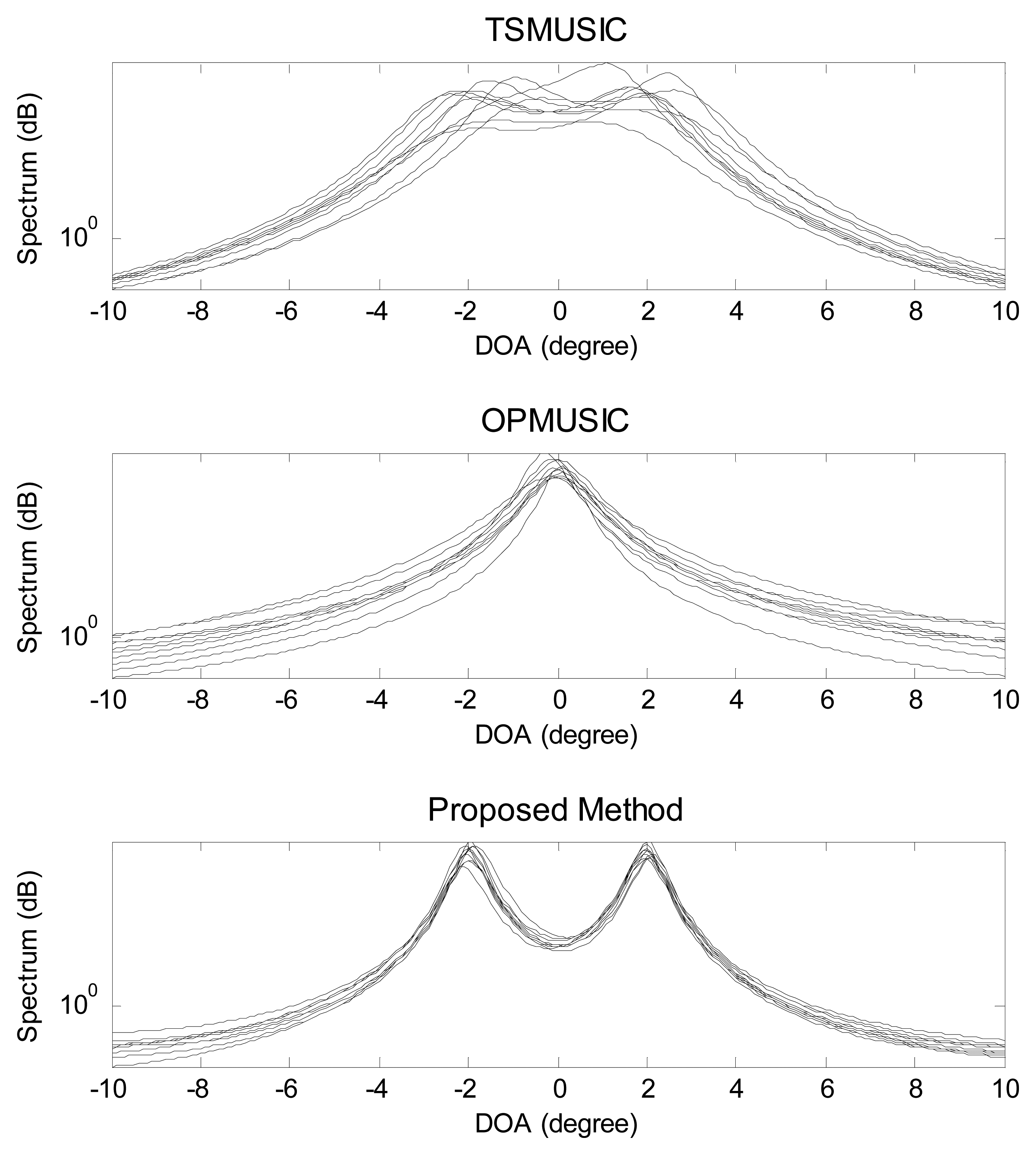
In the second experiment, the scenario of coexistence of one FFS and one NFS is investigated, with the location parameters being (θ₁ = − 2°,r₁ = 1.5λ) (NFS) and (θ₂ = 2°,r₂ = + ∞) (FFS). The snapshot number and the SNR equal to 500 and 5 dB, respectively. Ten independent trials of DOA spectrum estimates using the three methods are realized as is shown in Figure 3. It is obvious that, for the proposed method, there are two distinct peaks corresponding to the actual DOAs of the two mixed sources. However, TSMUSIC and OPMUSIC fails to distinguish the two closely spaced angles θ₁ and θ₂. This is because that, for closely spaced sources, it is very difficult for the subspace-based algorithms to correctly identify the signal subspace and noise subspace with low SNR, while the proposed method does not need any decomposition and identification of the subspaces.

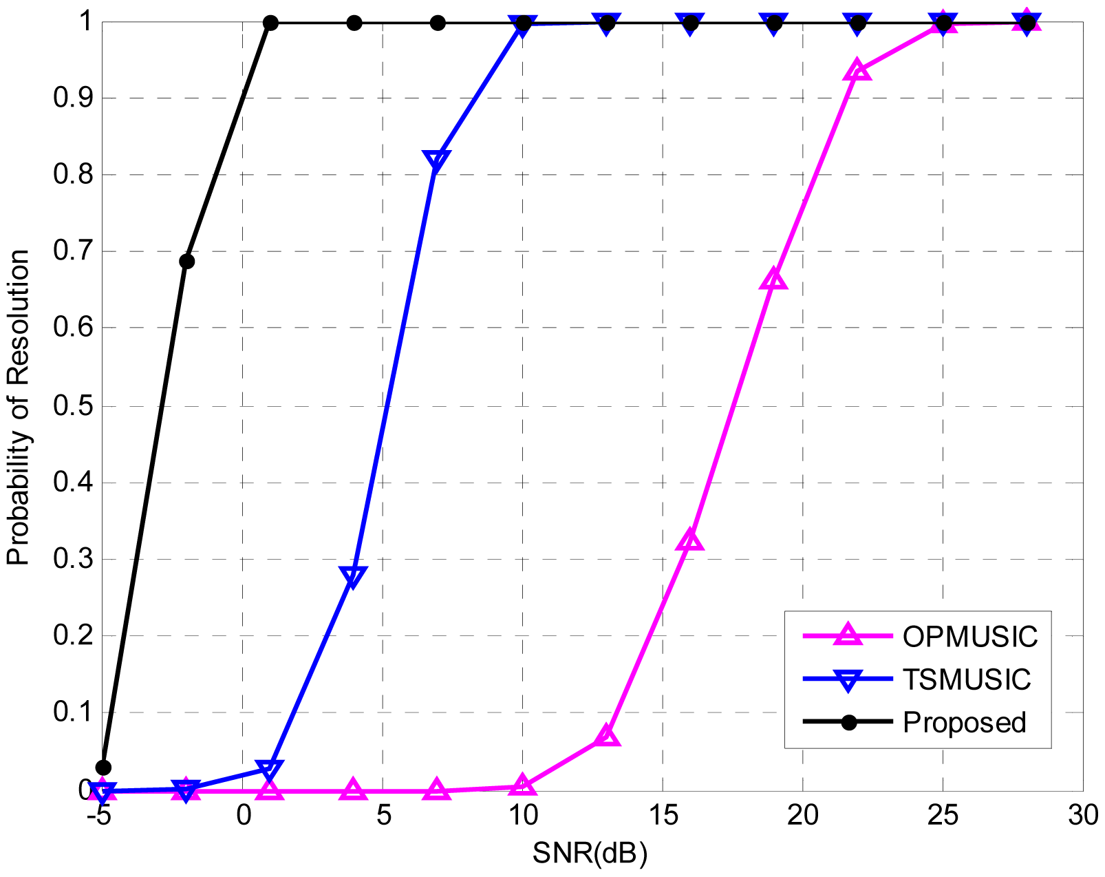
In the third experiment, the PR of the three algorithms versus SNR is explored. Consider two uncorrelated equi-power sources locating at (θ₁ = − 2°,r₁ = 1.5λ) (NFS) and (θ₂ = 2°,r₂ = +∞) (FFS), with number of snapshots being 500. The SNR varies from −5 dB to 28 dB in steps of 3 dB. At each SNR, 500 independent Monte Carlo trials are performed. Figure 4 illustrates the PR of the three algorithms as a function of SNR. It is obvious that the proposed method has the best resolution ability since it reaches a full PR at the lowest SNR threshold (1dB). For TSMUSIC and OPMUSIC, the SNR thresholds of full PR are 10 dB and 25 dB, respectively, which are much higher than that of our method. This is due to the fact that TSMUSIC and OPMUSIC suffer from the leakage between the signal subspace and noise subspace when SNR is low, while the subspace decomposition is not required in our algorithm, which promotes the resolution ability at low SNRs. Moreover, OPMUSIC has the worst resolution ability since its DOA estimator has a half aperture loss, while the array size is fully utilized in TSMUSIC and our method.

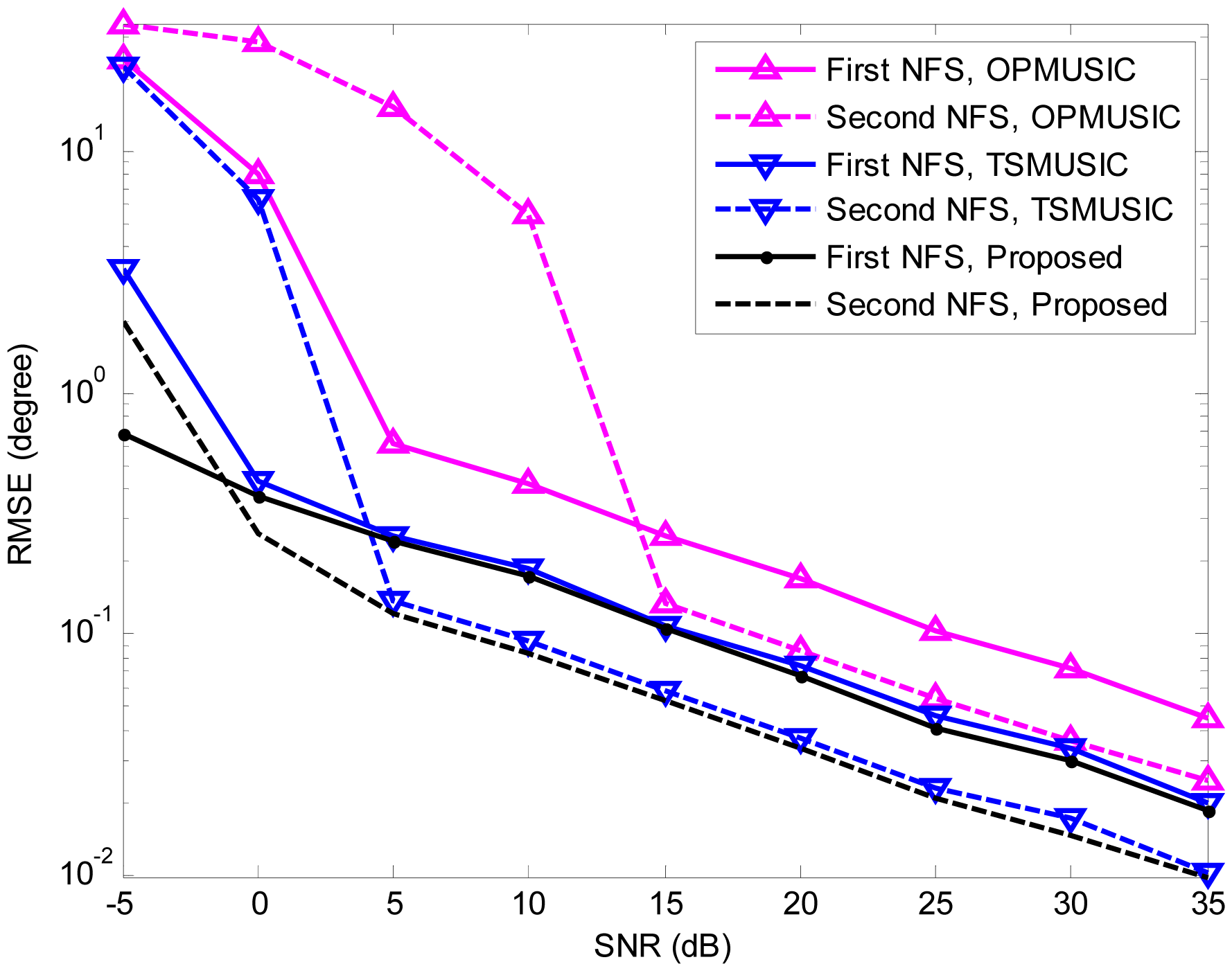
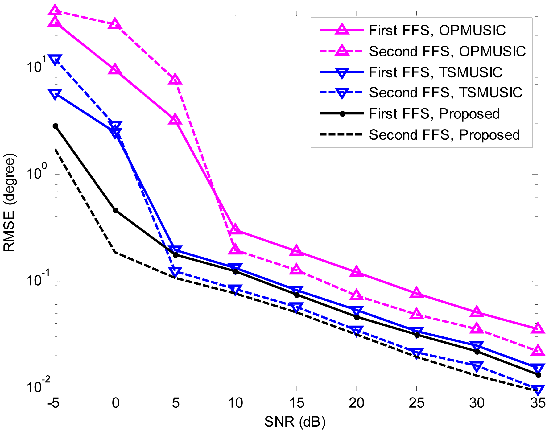
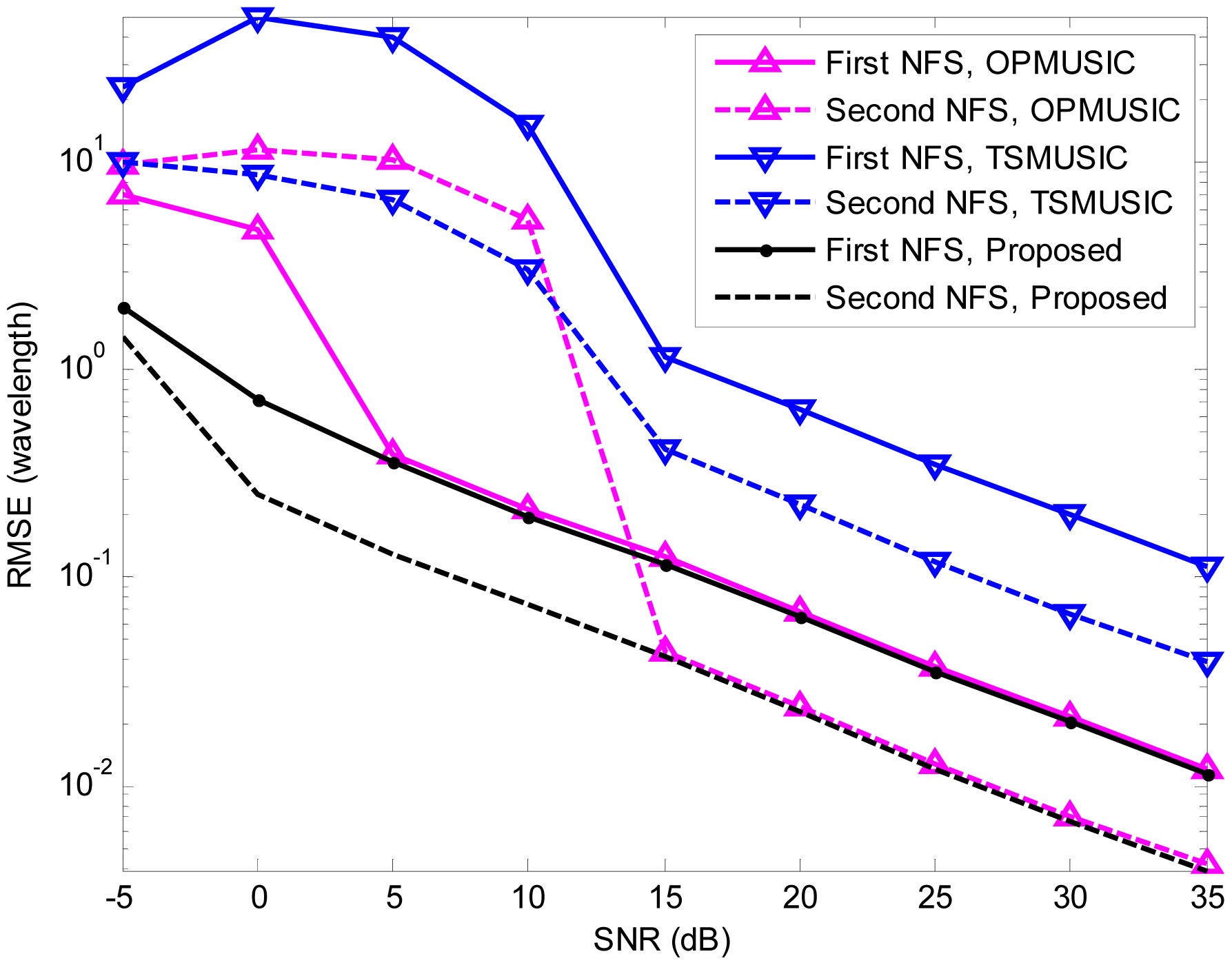
In the fourth experiment, we study the estimation accuracy of the three algorithms as a function of SNR. A more general mixed sources scenario is considered, where two FFSs are located at (θ₁ = 10°,r₁ = +∞), (θ₂ = 50°,r₂ = +∞), and two NFSs are placed at (θ₃ = − 10°,r₃ = 1.5λ), (θ₄ = − 30°,r₄ = 3λ) (θ₄ = − 30°,r₄ = 3λ), respectively. The SNR varies from −5 dB to 35 dB in steps of 5 dB, and the snapshot number is fixed at 200. At each SNR, 500 independent Monte Carlo trials are performed. Figures 5, 6 and 7 illustrate the RMSEs of DOA and range estimates using the three algorithms. It can be seen that the estimation accuracy (both DOA and range) of the proposed algorithm outperforms that of TSMUSIC and OPMUSIC, especially in the low SNR region. This can be also explained from the fact that incorrect identifications of signal subspaces are likely occur at low SNRs, which would deteriorate the performance of TSMUSIC and OPMUSIC. At the high SNR region, the DOA estimation accuracy of TSMUSIC approaches to that of our method, which is in agreement with the analysis presented in Section 4. OPMUSIC has the worst DOA estimation accuracy because of its half aperture loss. As for the range estimation, in the low SNR region, the proposed algorithm is still superior to TSMUSIC and OPMUSIC, which is mainly a result of the propagation error from the previous DOA estimation stage. In the high SNR region, however, OPMUSIC and our method have almost the same performance. Additionally, TSMUSIC has the worst range estimation performance since it only utilizes the information of a single eigenvector with the smallest eigenvalue to obtain the range estimates. As is described in [15], the DOA estimates and the range estimates are obtained from two different stages in TSMUSIC. In the first stage, a special cumulant matrix is constructed and decomposed. DOAs can be obtained via high resolution MUSIC algorithm. In the second stage, another particular cumulant matrix is constructed to avoid the estimation failure problem. However, it only utilizes the information of a single eigenvector with the smallest eigenvalue to obtain the range estimates in this stage. Therefore, TSMUSIC has a good performance in bearing estimation but a worst performance in range estimation in the simulations.

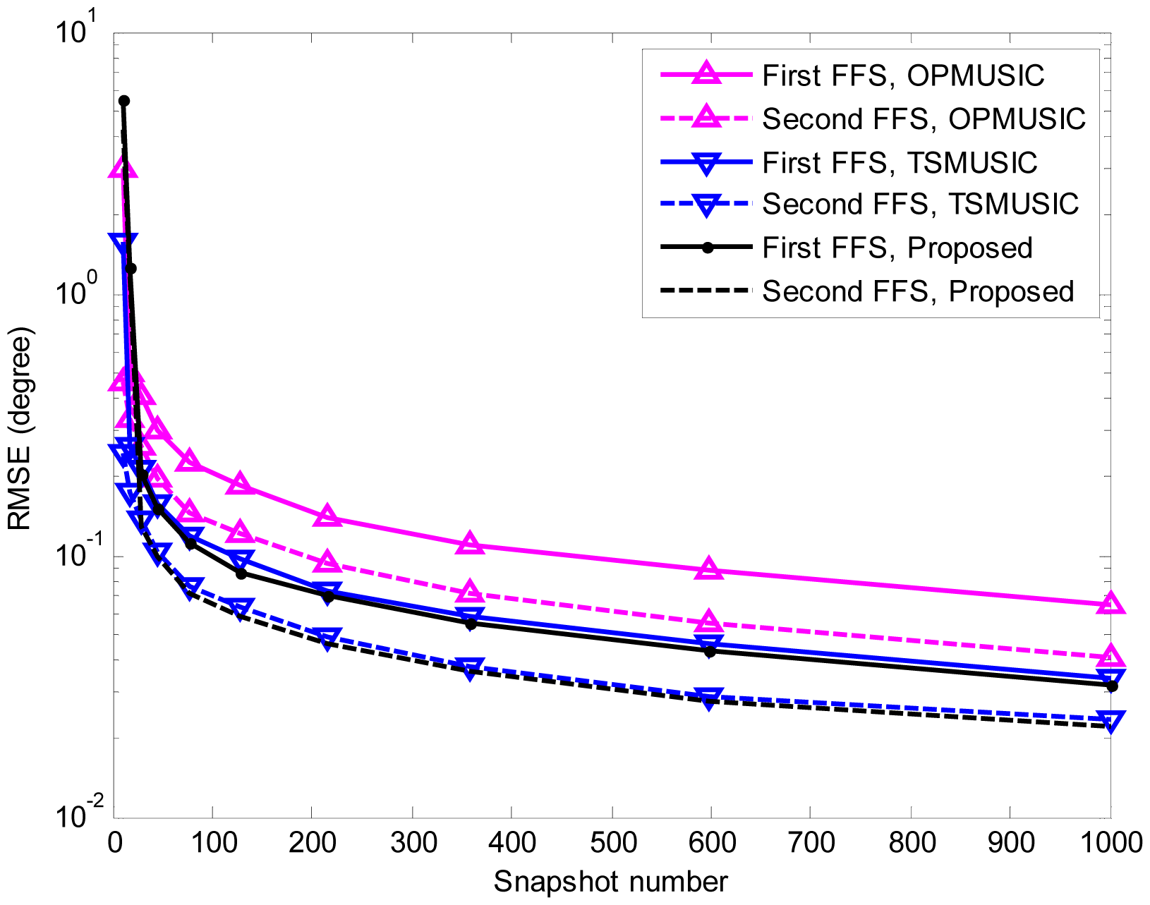
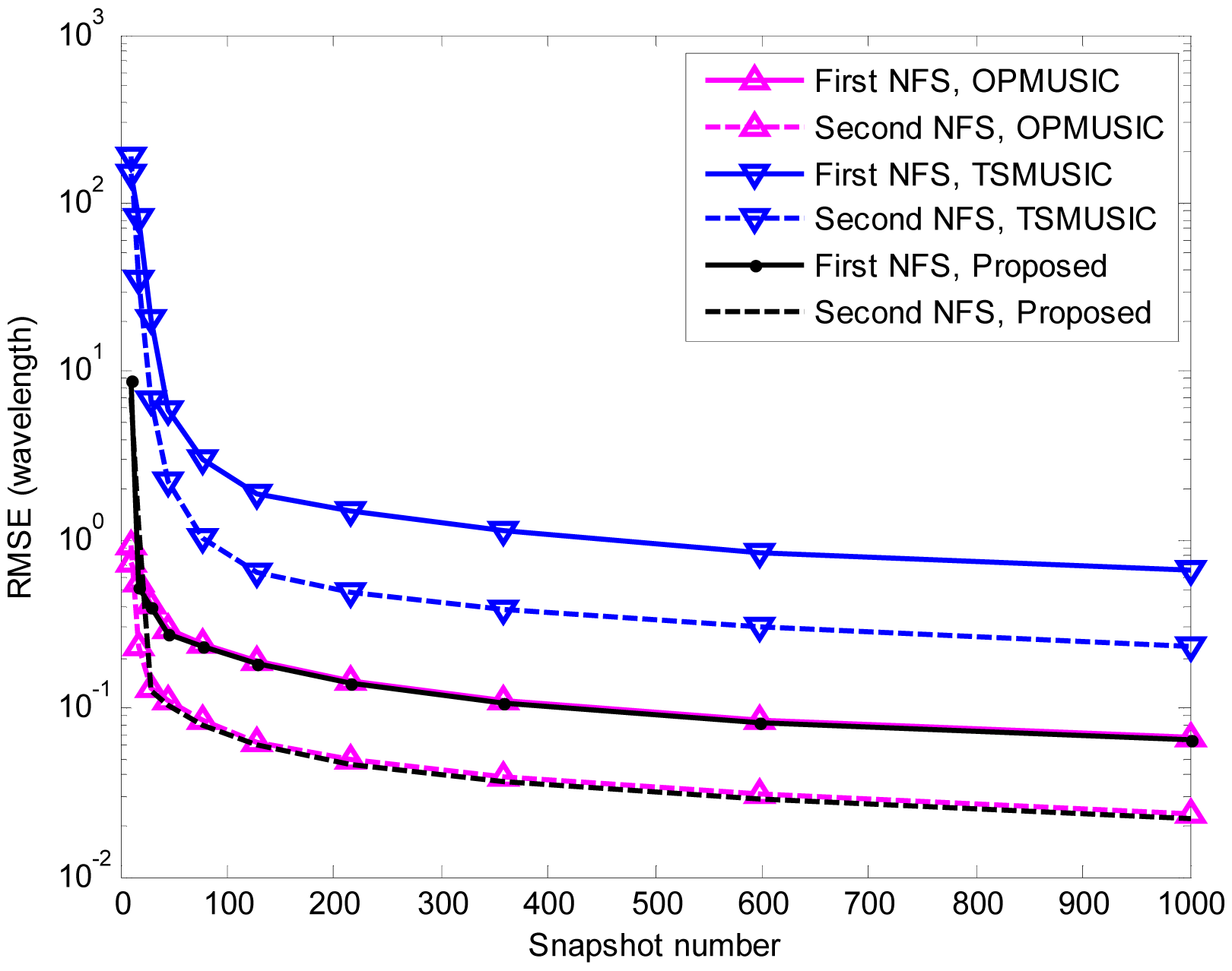
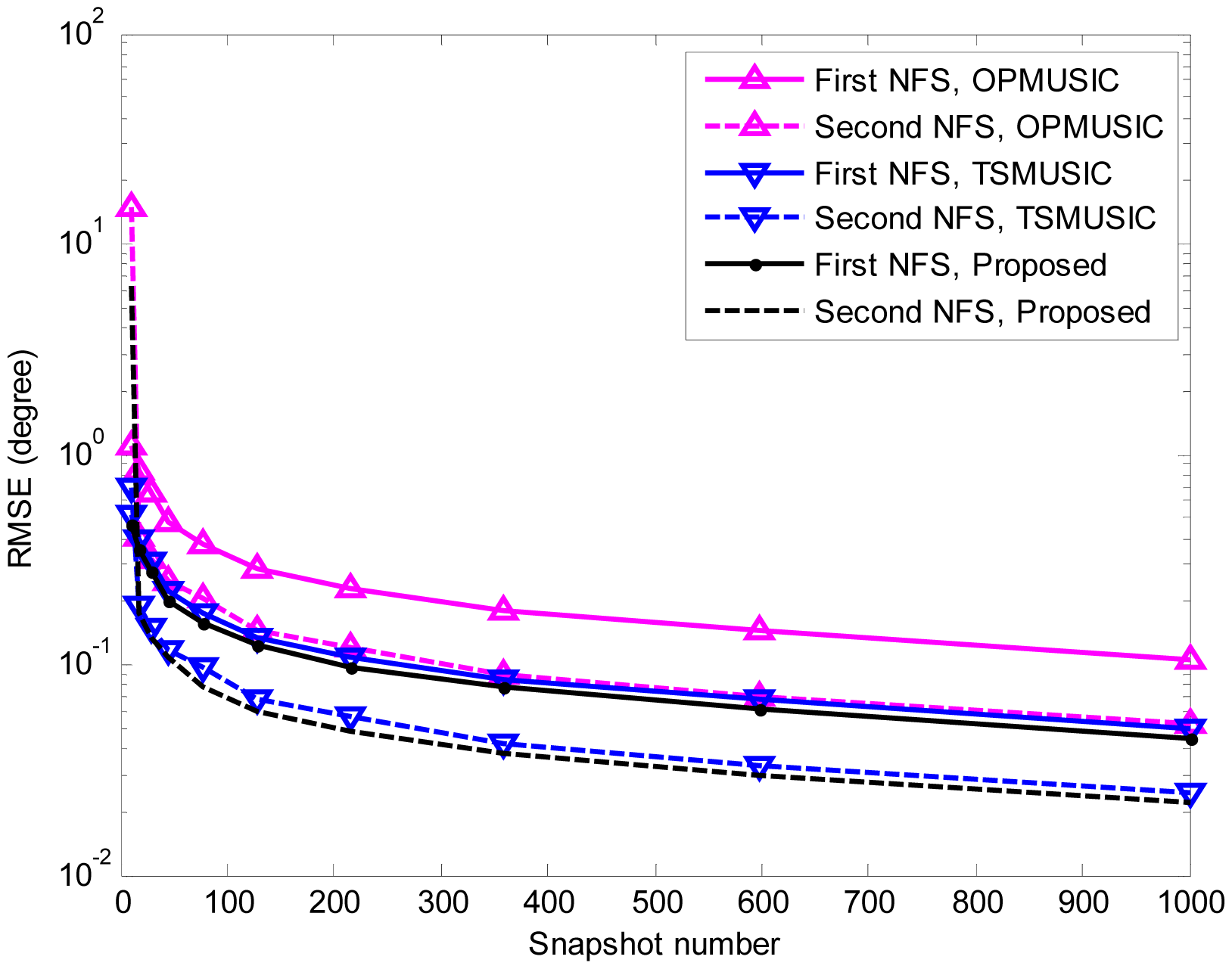
In the fifth experiment, the same parameters as the third experiment are adopted except that the SNR is set equal to 15 dB, and the number of snapshots varies from 10 to 1000. At each snapshot number, 500 independent Monte Carlo trials are performed. The RMSEs of DOA and range estimation are shown in Figure 8, 9 and 10. It is obvious that the RMSEs (both DOA and range) of the three algorithms decrease monotonically as the snapshot number increases. This is due to the fact that a larger sampling number will produce better estimate of the cumulant matrices and the covariance matrices for stationary data. Furthermore, when the snapshot number is large enough, the proposed algorithm slightly outperforms TSMUSIC and OPMUSIC. This is because that: (1) the array aperture is fully utilized in this algorithm; (2) both the temporal and spatial structures of the observed data are utilized in our method, which also contribute to the improvement of estimation accuracy. However, when the sample size is small (i.e., snapshot number = 10), the DOA estimation accuracy of our method is a little bit inferior to that of TSMUSIC and OPMUSIC. This can be explained that the estimation of the spatial-temporal cumulant matrices is not reliable when the sample size is insufficient.

In the last experiment, we compare the computational complexity of the three algorithms. Suppose that there are 2M + 1 = 9 sensors, and that the searching steps θ_Δ and r_Δ are set as 0.1° and 0.05λ, respectively. The number of snapshots varies from 10 to 1000. Furthermore, we define K = 2 and L = 5. Figure 11 illustrates the computational burden of these algorithms as a function of the snapshot number. It is clear that the proposed algorithm has slightly higher complexity than TSMUSIC, while OPMUSIC is most efficient in computational complexity since it only involves second-order statistics.

7. Conclusions

In this paper, a novel algorithm has been proposed for the localization of mixed FFSs and NFSs. Based on the joint diagonalization structure of multiple fourth-order spatial-temporal cumulant matrices and the beamforming technique, the DOA and range parameters of FFSs and NFSs have been determined respectively. Compared with some existing mixed source localization methods, the new method has the main advantage that it does not require the information of the source number. Such an advantage is practically attractive since mixed source enumeration is typically a very difficult problem. In addition, we have found that our method is a generalization of the TSMUSIC algorithm in [15], which only utilize one single spatial-temporal cumulant matrix. Moreover, the proposed algorithm avoids multidimensional search, aperture loss and parameter matching. According to the simulation results, the proposed method outperforms TSMUSIC and OPMUSIC in both resolution ability and estimation accuracy, especially when the SNR is low.

It is worth mentioning that there are two slight limitations of the proposed algorithm. First, the construction of cumulant matrices leads to high computational load. Second, it is limited to localize mixed sources only in the 2-D domain (elevation angle and range). To put the proposed algorithm into further applications, several steps of the future work can be shown as follows:

• To reduce the computational complexity, second-order statistics and real-valued transformation may be applied.

• To extend the proposed algorithm for joint azimuth-elevation-range (3-D) estimation problem, we may employ planar arrays, such as cross array, rectangular array and circular array.

References

- Krim, H.; Viberg, M. Two decades of array signal processing research: The parametric approach. IEEE Signal Process. Mag. 1996, 13, 67–94. [Google Scholar]
- Schmidt, R.O. Multiple emitter location and signal parameter estimation. IEEE Trans. Antennas Propag. 1986, 34, 276–280. [Google Scholar]
- Roy, R.; Kailath, T. ESPRIT-estimation of signal parameters via rotational invariance techniques. IEEE Trans. Acoust. Speech Signal Process. 1989, 37, 984–995. [Google Scholar]
- Zoltowski, M.D.; Kautz, G.M.; Silverstein, S.D. Beamspace Root-MUSIC for minimum redundancy linear arrays. IEEE Trans. Signal Process. 1993, 41, 2502–2507. [Google Scholar]
- Haardt, M.; Nossek, J.A. Unitary ESPRIT: How to obtain increased estimation accuracy with a reduced computational burden. IEEE Trans. Signal Process. 1995, 43, 1232–1242. [Google Scholar]
- Pesavento, M.; Gershman, A.B.; Haardt, M. Unitary root-MUSIC with a real-valued eigendecomposition: A theoretical and experimental performance study. IEEE Trans. Signal Process. 2000, 48, 1306–1314. [Google Scholar]
- Johnson, R.C. Antenna Engineering Handbook, 3rd ed.; McGraw-Hill: New York, NY, USA, 1993; pp. 26–29. [Google Scholar]
- Huang, Y.; Barkat, M. Near-field multiple source localization by passive sensor array. IEEE Trans. Antennas Propag. 1991, 39, 968–975. [Google Scholar]
- Lee, J.; Chen, Y.; Yeh, C. A covariance approximation method for near-field direction-finding using a uniform linear array. IEEE Trans. Signal Process. 1995, 43, 1293–1298. [Google Scholar]
- Noh, H.; Lee, C. A covariance approximation method for near-field coherent sources localization using uniform linear array. IEEE J. Ocean. Eng. 2013, 38, 1–9. [Google Scholar]
- Grosicki, E.; Abed-Meraim, K.; Hua, Y. A weighted linear prediction method for near-field source localization. IEEE Trans. Signal Process. 2005, 53, 3651–3660. [Google Scholar]
- Zhi, W.; Chia, M.Y.W. Near-field source localization via symmetric subarrays. IEEE Signal Process. Lett. 2007, 14, 409–412. [Google Scholar]
- Tao, J.; Liu, L.; Lin, Z. Joint DOA, range, and polarization estimation in the fresnel region. IEEE Trans. Aerosp. Electron. Syst. 2011, 47, 2657–2672. [Google Scholar]
- He, J.; Ahmad, M.O.; Swamy, M. Near-field localization of partially polarized sources with a cross-dipole array. IEEE Trans. Aerosp. Electron. Syst. 2013, 49, 857–870. [Google Scholar]
- Liang, J.; Liu, D. Passive localization of mixed near-field and far-field sources using two-stage MUSIC algorithm. IEEE Trans. Signal Process. 2010, 58, 108–120. [Google Scholar]
- He, J.; Swamy, M.; Ahmad, M.O. Efficient application of MUSIC algorithm under the coexistence of far-field and near-field sources. IEEE Trans. Signal Process. 2012, 60, 2066–2070. [Google Scholar]
- Liu, G.; Sun, X.; Liu, Y.; Qin, Y. Low-complexity estimation of signal parameters via rotational invariance techniques algorithm for mixed far-field and near-field cyclostationary sources localisation. IET Signal Process. 2013, 7, 382–388. [Google Scholar]
- Wang, B.; Zhao, Y.; Liu, J. Mixed-order MUSIC algorithm for localization of far-field and near-field sources. IEEE Signal Process. Lett. 2013, 20, 311–314. [Google Scholar]
- Gao, F.; Gershman, A.B. A generalized ESPRIT approach to direction-of-arrival estimation. IEEE Signal Process. Lett. 2005, 12, 254–257. [Google Scholar]
- Liu, G.; Sun, X. Spatial differencing method for mixed far-field and near-field sources localization. IEEE Signal Process. Lett. 2014, 21, 1331–1335. [Google Scholar]
- Liu, G.; Sun, X. Two-stage matrix differencing algorithm for mixed far-field and near-field sources classification and localization. IEEE Sens. J. 2014, 14, 1957–1965. [Google Scholar]
- Liu, G.; Sun, X. Efficient method of passive localization for mixed far-field and near-field sources. IEEE Antennas Wirel. Propag. Lett. 2013, 12, 902–905. [Google Scholar]
- Jiang, J.; Duan, F.; Chen, J.; Li, Y.; Hua, X. Mixed near-field and far-field sources localization using the uniform linear sensor array. IEEE Sens. J. 2013, 13, 3136–3143. [Google Scholar]
- Xie, J.; Tao, H.; Rao, X.; Su, J. Comments on “Near-Field Source Localization via Symmetric Subarrays”. IEEE Signal Process. Lett. 2015, 22, 643–644. [Google Scholar]
- Tian, Y.; Sun, X. Passive localization of mixed sources jointly using MUSIC and sparse signal reconstruction. Aeu-Int. J. Electron. C. 2014, 68, 534–539. [Google Scholar]
- Tian, Y.; Sun, X. Mixed sources localisation using a sparse representation of cumulant vectors. IET Signal Process. 2014, 8, 382–388. [Google Scholar]
- Wang, B.; Liu, J.; Sun, X. Mixed sources localization based on sparse signal reconstruction. IEEE Signal Process. Lett. 2012, 19, 487–490. [Google Scholar]
- Jiang, J.; Duan, F.; Chen, J. Three-dimensional localization algorithm for mixed near-field and far-field sources based on ESPRIT and MUSIC method. Prog. Electromagn. Res. 2013, 136, 435–456. [Google Scholar]
- Liang, J.; Liu, D.; Zeng, X.; Wang, W.; Zhang, J.; Chen, H. Joint azimuth-elevation/(-range) estimation of mixed near-field and far-field sources using two-stage separated steering vector-based algorithm. Prog. Electromagn. Res. 2011, 113, 17–46. [Google Scholar]
- Huang, Q.; Wang, T. Acoustic source localization in mixed field using spherical microphone arrays. EURASIP J. Adv. Signal Process. 2014, 2014, 1–16. [Google Scholar]
- Akaike, H. A new look at the statistical model identification. IEEE Trans. Autom. Control 1974, 19, 716–723. [Google Scholar]
- Wax, M.; Kailath, T. Detection of signals by information theoretic criteria. IEEE Trans. Acoust. Speech Signal Process. 1985, 33, 387–392. [Google Scholar]
- Djuric, P.M. A model selection rule for sinusoids in white Gaussian noise. IEEE Trans. Signal Process. 1996, 44, 1744–1751. [Google Scholar]
- Van, J. TIME-MUSIC DOA estimation based on the exploitation of an arbitrary-order temporal structure in the data. Proceedings of Sensor Array and Multichannel Signal Processing Workshop; pp. 308–312.
- Capon, J. High-resolution frequency-wavenumber spectrum analysis. Proc. IEEE. 1969, 57, 1408–1418. [Google Scholar]
- Wolfel, M.; McDonough, J. Minimum variance distortionless response spectral estimation. IEEE Signal Process. Mag. 2005, 22, 117–126. [Google Scholar]