
Event Coverage Detection and Event Source Determination in Underwater Wireless Sensor Networks

Abstract
:1. Introduction
- Our sub-region query processing mechanism developed in [22] has been improved, where a set of neighboring sensor nodes, whose sensory data deviate from a normal sensing range in a collective fashion, are identified. These sensory data are routed to sink node(s) through our routing tree [22] in an energy-efficient fashion.
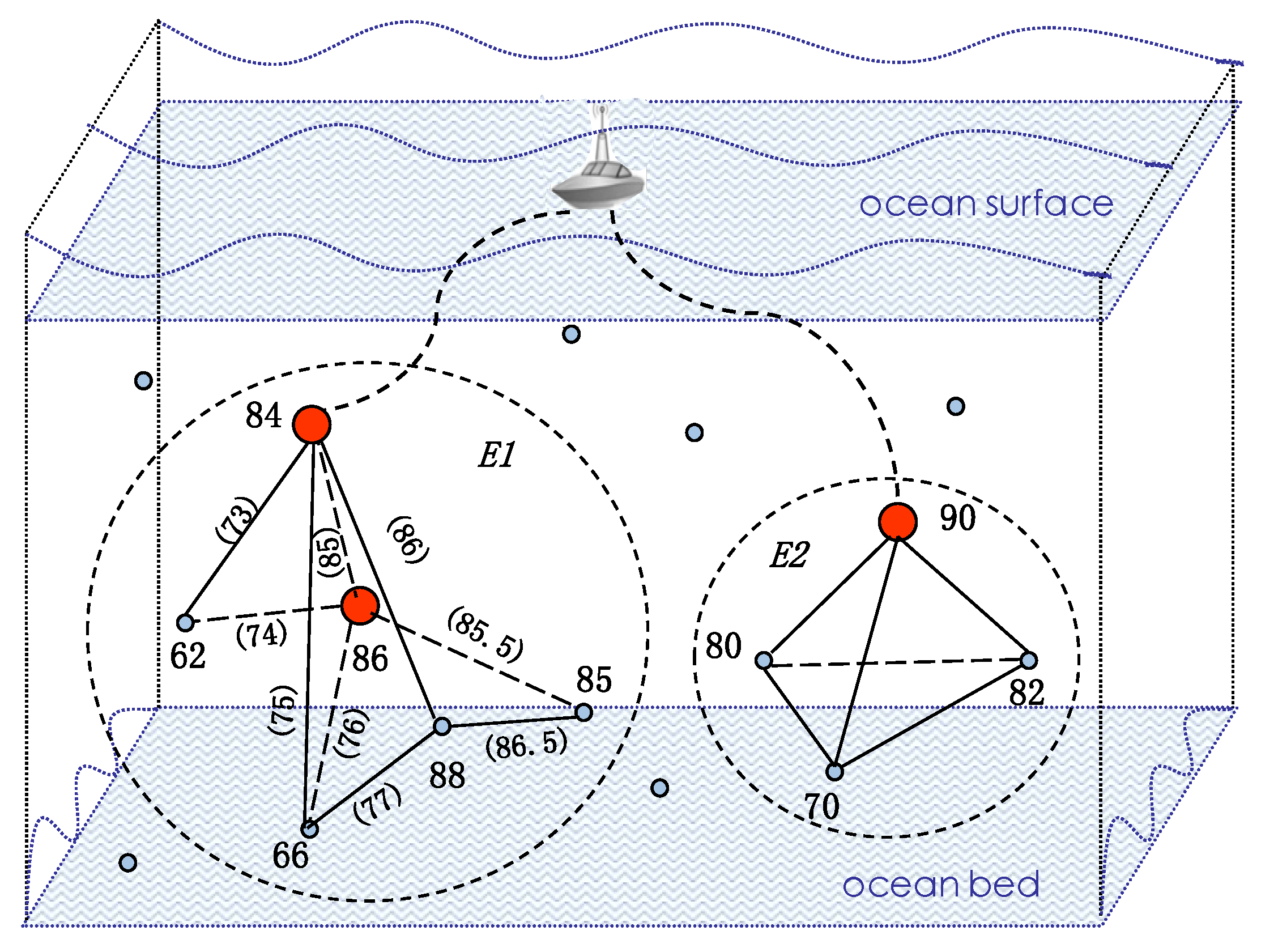
- Based on the sensory data of sensor nodes in possible event regions, the coverage of events is detected, which is represented as a network (or a weighted graph) of sensor nodes. Potential event sources are determined through an algorithm that identifies barycenters in a weighted graph [25]. Generally, an event source can be identified as a barycenter in the graph of sensor nodes, whose sensory data deviate the most in value with respect to a normal sensing range.
- Extensive simulations have been conducted to evaluate the effectiveness and efficiency of our event coverage detection and event source determination mechanisms. The results show that our technique is more energy efficient, especially when the network topology is relatively steady.
2. Preliminaries: Routing Tree Construction and Maintenance
3. Event Detection and Sensory Data Aggregation
- HC() = HC(), for the case that ∈ , or HC() = (HC() − 1), for the case that ∈ . This means that is not farther from SN in hop count compared to . Therefore, the strategy that relays sensory data for may consume less, or no more in the worst case, energy than the strategy that relays sensory data for .
- When tag for is 1 (Line 2), which means that sensory data for deviates from a normal sensing range and should be routed to SN. In this case, if there is another sensor node , whose sensory data deviates from a normal sensing range, as well, and should be relayed to SN by , can be a candidate relay node for .
- When tag for is 0 (line 2), which means that sensory data for is within a normal sensing range. In this case, if there are no less than two sensor nodes whose sensory data deviate from a normal sensing range and should be relayed to SN by , can be a candidate relay node for forwarding sensory data of these sensor nodes.
| Algorithm 1 Response for control packets. |
Require:
|
Ensure:
|
|
- relay sensory data for a larger number of sensor nodes, which may reduce the number of sensory data packets to be forwarded in the network, or
- have more remaining energy with respect to its hop count (reflected by . ÷ .), which may promote the balance of energy consumption between sensor nodes and, thus, prolong the network lifetime.It is worth noting that when (i) the condition . ≥ . holds, which means that . is not nearer SN in hop count in comparison with ., but (ii) the condition . ÷ . > . ÷ . holds, which means that . can forward a larger number of sensory data packets than ., . is assumed more appropriate than . to serve as the relay node,
| Algorithm 2 Relay node selection. |
Require:
|
Ensure:
|
|
| Algorithm 3 Sensory data gathering and aggregation. |
Require:
|
Ensure:
|
|
4. Event Coverage Detection and Event Sources Determination
| Algorithm 4 Event coverage detection. |
Require:
|
Ensure:
|
|

| Algorithm 5 Event source determination. |
Require:
|
Ensure:
|
|
- there exists slots for candidate event sources (Lines 8–9) or
- there exists another candidate event source (Line 11), which is not as appropriate as (Line 12). This is specified by the condition of . < .. Consequently, is replaced by in (Line 13).
5. Implementation and Evaluation
5.1. Environment Settings
5.2. Experimental Evaluation

| Parameter Name | Value |
|---|---|
| Simulation network region (km) | 1 × 2 × |
| Number of sensor nodes (including one sink node) | 61 |
| Transmission radius r (km) | |
| Time slots for experiments | 10, 20, 30 |
| EPING or control packet size (B) | 11 |
| EPONG or HELLO control packet size (B) | 7 |
| ACK and getData control packet size (B) | 6 |
| Data packet payload size (B) | 100 |
| Robustness factor for the parent-child relation determination | |
| Smoothing factor for the link quality computation | |
| Power for transmitting a data packet (W) | |
| Power for transmitting a control packet (W) |


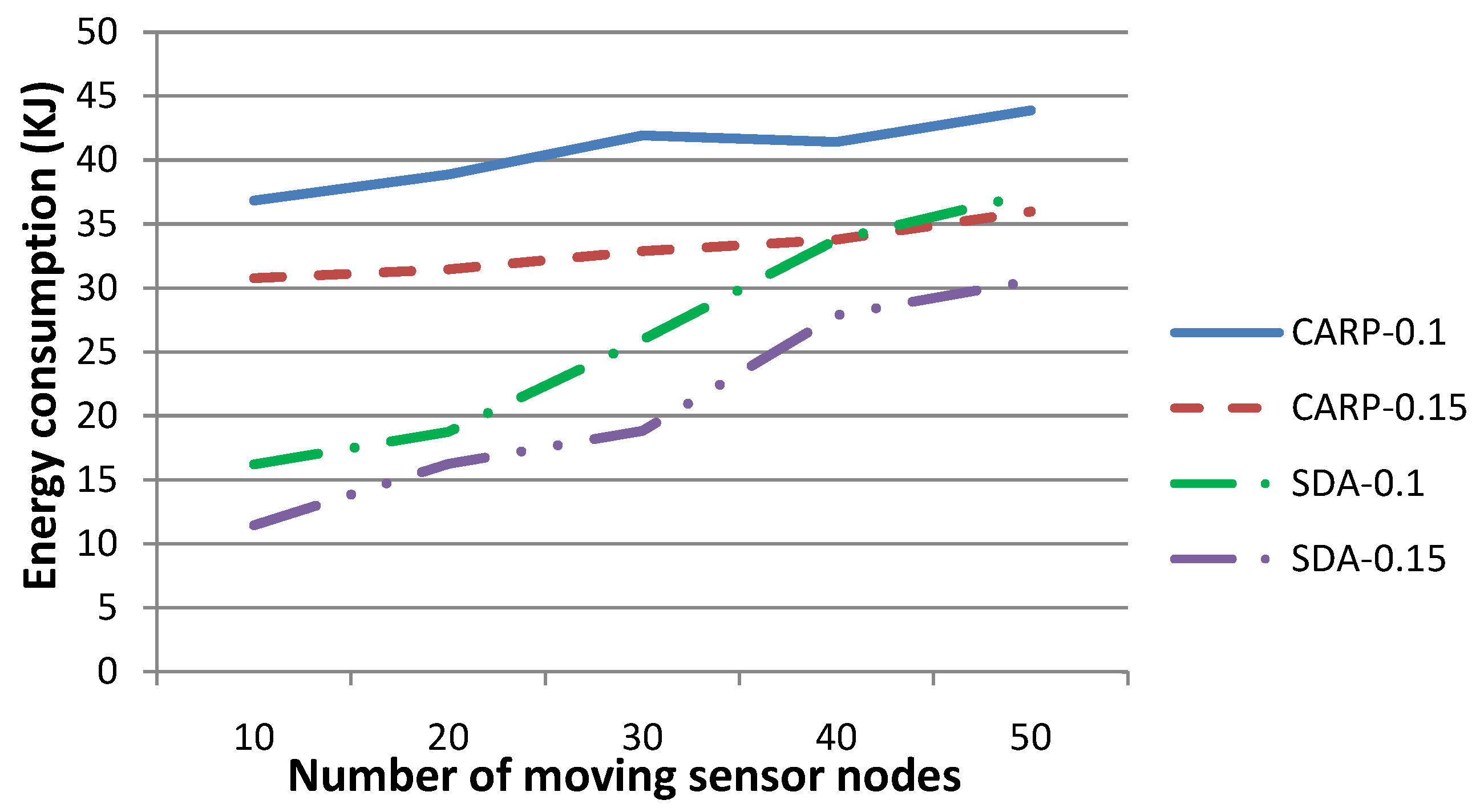
5.3. Comparison with CARP for the Number of Control Packets and Energy Consumption


6. Related Work and Comparison
7. Conclusions
Acknowledgments
Author Contributions
Conflicts of Interest
References
- Fang, S.; Xu, L.D.; Zhu, Y.; Ahati, J.; Pei, H.; Yan, J.; Liu, Z. An Integrated System for Regional Environmental Monitoring and Management Based on Internet of Things. IEEE Trans. Ind. Inf. 2014, 10, 1596–1605. [Google Scholar] [CrossRef]
- Climent, S.; Sanchez, A.; Capella, J.V.; Meratnia, N.; Serrano, J.J. Underwater Acoustic Wireless Sensor Networks: Advances and Future Trends in Physical, MAC and Routing Layers. Sensors 2014, 14, 795–833. [Google Scholar] [CrossRef] [PubMed]
- Ayaz, M.; Baig, I.; Abdullah, A.; Faye, I. A survey on routing techniques in underwater wireless sensor networks. J. Netw. Comput. Appl. 2011, 34, 1908–1927. [Google Scholar] [CrossRef]
- Kaiser, S.A. Legal considerations about the missing malaysia airlines flight MH 370. Air Space Law 2014, 39, 235–244. [Google Scholar]
- Zuba, M. Connecting with Oceans Using Underwater Acoustic Networks. XRDS Crossroads ACM Mag. Stud. 2014, 20, 32–37. [Google Scholar] [CrossRef]
- Yan, H.; Shi, Z.J.; Cui, J.H. DBR: Depth-Based Routing for Underwater Sensor Networks. In Proceedings of the 7th International IFIP-TC6 Networking Conference on Ad Hoc and Sensor Networks, Wireless Networks, Next Generation Internet, Singapore, 5–9 May 2008; pp. 72–86.
- Domingo, M.C. An overview of the internet of underwater things. J. Netw. Comput. Appl. 2012, 35, 1879–1890. [Google Scholar] [CrossRef]
- Xu, G.; Shen, W.; Wang, X. Applications of Wireless Sensor Networks in Marine Environment Monitoring: A Survey. Sensors 2014, 14, 16932–16954. [Google Scholar] [CrossRef] [PubMed]
- Umar, A.; Javaid, N.; Ahmad, A.; Khan, Z.A.; Qasim, U.; Alrajeh, N.; Hayat, A. DEADS: Depth and Energy Aware Dominating Set Based Algorithm for Cooperative Routing along with Sink Mobility in Underwater WSNs. Sensors 2015, 15, 14458–14486. [Google Scholar] [CrossRef] [PubMed]
- Akhlaq, M.; Sheltami, T.R.; Shakshuki, E.M. C3: An energy-efficient protocol for coverage, connectivity and communication in WSNs. Pers. Ubiquit. Comput. 2014, 18, 1117–1133. [Google Scholar] [CrossRef]
- Adnan, T.; Datta, S.; MacLean, S. Efficient and accurate sensor network localization. Pers. Ubiquit. Comput. 2014, 18, 821–833. [Google Scholar] [CrossRef]
- Han, G.; Zhang, C.; Shu, L.; Rodrigues, J.J.P.C. Impacts of Deployment Strategies on Localization Performance in Underwater Acoustic Sensor Networks. IEEE Trans. Ind. Electron. 2015, 62, 1725–1733. [Google Scholar] [CrossRef]
- Burguera, A.; Bonin-Font, F.; Oliver, G. Trajectory-Based Visual Localization in Underwater Surveying Missions. Sensors 2015, 15, 1708–1735. [Google Scholar] [CrossRef] [PubMed]
- Noh, Y.; Lee, U.; Lee, S.; Wang, P.; Vieira, L.F.M.; Cui, J.H.; Gerla, M.; Kim, K. HydroCast: Pressure Routing for Underwater Sensor Networks. IEEE Trans. Veh. Technol. 2015. [Google Scholar] [CrossRef]
- Cho, H.H.; Chen, C.Y.; Shih, T.K.; Cha, H.C. Survey on underwater delay/disruption tolerant wireless sensor network routing. IET Wirel. Sens. Syst. 2014, 4, 112–121. [Google Scholar] [CrossRef]
- Lloret, J. Underwater Sensor Nodes and Networks. Sensors 2013, 13, 11782–11796. [Google Scholar] [CrossRef] [PubMed]
- Wang, Z.; Liu, M.; Zhang, S.; Qiu, M. Sensor virtualization for underwater event detection. J. Syst. Archit. 2014, 60, 619–629. [Google Scholar] [CrossRef]
- Zhou, H.; Xia, S.; Jin, M.; Wu, H. Localized and Precise Boundary Detection in 3-D Wireless Sensor Networks. IEEE/ACM Trans. Netw. 2015. [Google Scholar] [CrossRef]
- OReilly, C.; Gluhak, A.; Imran, M.A.; Rajasegarar, S. Anomaly Detection in Wireless Sensor Networks in a Non-Stationary Environment. IEEE Commun. Surv. Tutor. 2014, 16, 1413–1432. [Google Scholar] [CrossRef]
- Kundu, S.; Das, N. Event Boundary Detection and Gathering in Wireless Sensor Networks. In Proceedings of the IEEE Conference on Applications and Innovations in Mobile Computing, Kolkata, India, 12–14 February 2015; pp. 62–67.
- Debont, M.; Jamshaid, K.; Shihada, B.; Ho, P.H. Event Localization in Underwater Wireless Sensor Networks using Monitoring Courses. In Proceedings of the IEEE International Conference on Communications in China: Wireless Networking and Applications, Beijing, China, 15–17 August 2012; pp. 769–774.
- Zhou, Z.; Xing, R.; Gaaloul, W.; Xiong, Y. A Three-Dimensional Sub-Region Query Processing Mechanism in Underwater WSNs. Pers. Ubiquit. Comput. 2015, 19, 1075–1086. [Google Scholar] [CrossRef]
- Han, G.; Jiang, J.; Shu, L.; Xu, Y.; Wang, F. Localization Algorithms of Underwater Wireless Sensor Networks: A Survey. Sensors 2012, 12, 2026–2061. [Google Scholar] [CrossRef] [PubMed]
- King, K.; Nittel, S. Efficient Data Collection and Event Boundary Detection in Wireless Sensor Networks Using Tiny Models. In Proceedings of the 6th International Conference on Geographic Information Science, Zurich, Switzerland, 14–17 September 2010; pp. 100–114.
- Cohen, J. Barycentric Graph Clustering. Oregon Health Science University 2008. [Google Scholar]
- Emokpae, L.E.; Benedetto, S.D.; Potteiger, B.; Younis, M. UREAL: Underwater Reflection-Enabled Acoustic-Based Localization. IEEE Sens. J. 2014, 14, 3915–3925. [Google Scholar] [CrossRef]
- Basagni, S.; Petrioli, C.; Petroccia, R.; Spaccini, D. CARP: A Channel-aware routing protocol for underwater acoustic wireless networks. Ad Hoc Netw. 2015, 34, 92–104. [Google Scholar] [CrossRef]
- Coutinho, R.W.L.; Boukerche, A.; Vieira, L.F.M.; Loureiro, A.A.F. GEDAR: Geographic and Opportunistic Routing Protocol with Depth Adjustment for Mobile Underwater Sensor Networks. In Procedings of the IEEE International Conference on Communications, Sydney, NSW, Australia, 10–14 June 2014; pp. 251–256.
- Shin, D.; Hwang, D.; Kim, D. DFR: An efficient directional flooding-based routing protocol in underwater sensor networks. Wirel. Commun. Mob. Comput. 2012, 12, 1517–1527. [Google Scholar] [CrossRef]
- Bahrami, N.; Khamis, N.H.H.; Baharom, A. Study of Underwater Channel Estimation Based on Different Node Placement in Shallow Water. IEEE Sens. J. 2015. [Google Scholar] [CrossRef]
- Emokpae, L.E.; Younis, M. Surface-Reflection-Based Communication and Localization in Underwater Sensor Networks. ACM Trans. Sens. Netw. 2014, 10, 50. [Google Scholar] [CrossRef]
- Xu, M.; Liu, G. A Multi-Link Fault-Tolerant Routing Protocol for Three Dimensional Underwater Acoustic Sensor Networks. J. Comput. Inf. Syst. 2013, 9, 4345–4352. [Google Scholar]
- Zhou, Z.; Yao, B.; Xing, R.; Shu, L.; Bu, S. E-CARP: An Energy Efficient Routing Protocol for UWSNs in the Internet of Underwater Things. IEEE Sens. J. 2015. [Google Scholar] [CrossRef]
- Shahid, N.; Naqvi, I.H.; Qaisar, S.B. Characteristics and classification of outlier detection techniques for wireless sensor networks in harsh environments: A survey. Artif. Intell. Rev. 2015, 43, 193–228. [Google Scholar] [CrossRef]
- Zheng, H.; Wu, J. Data Collection and Event Detection in the Deep Sea with Delay Minimization. In Proceedings of the 12th Annual IEEE International Conference on Sensing, Communication and Networking, Seattle, WA, USA, 22–25 June 2015.
- Basagni, S.; Boloni, L.; Gjanci, P.; Petrioli, C.; Phillips, C.A.; Turgut, D. Maximizing the Value of Sensed Information in Underwater Wireless Sensor Networks via an Autonomous Underwater Vehicle. In Proceedings of the IEEE Conference on Computer Communications, Toronto, ON, Canada, 27 April–2 May 2014; pp. 988–996.
- Kim, Y.; Park, S.H. A Query Result Merging Scheme for Providing Energy Efficiency in Underwater Sensor Networks. Sensors 2011, 11, 11833–11855. [Google Scholar] [CrossRef] [PubMed]
- Huang, J.; Sun, L.; Wei, X.; Sun, P.; Huang, H.; Wang, R. Redundancy Model and Boundary Effects Based Coverage-Enhancing Algorithm for 3D Underwater Sensor Networks. Int. J. Distrib. Sens. Netw. 2014, 7, 234–244. [Google Scholar] [CrossRef]
- Jiang, P.; Wang, X.; Jiang, L. Node Deployment Algorithm Based on Connected Tree for Underwater Sensor Networks. Sensors 2015, 15, 16763–16785. [Google Scholar] [CrossRef] [PubMed]
- Amiri, Z.; Pouyan, A.A.; Mashayekhi, H. A topology control algorithm for autonomous underwater robots in three-dimensional space using PSO. J. AI Data Min. 2015, 3, 191–201. [Google Scholar]
- Guo, P.; Cao, J.; Zhang, K. Distributed Topological Convex Hull Estimation of Event Region in Wireless Sensor Networks without Location Information. IEEE Trans. Parall. Distrib. Syst. 2015, 26, 85–94. [Google Scholar] [CrossRef]
- Keally, M.; Zhou, G.; Xing, G.; Nguyen, D.T.; Qi, X. A Learning-Based Approach to Confident Event Detection in Heterogeneous Sensor Networks. ACM Trans. Sens. Netw. 2014, 11. [Google Scholar] [CrossRef]
- Alam, K.M.; Kamruzzaman, J.; Karmakar, G.; Murshed, M. Dynamic adjustment of sensing range for event coverage in wireless sensor networks. J. Netw. Comput. Appl. 2014, 46, 139–153. [Google Scholar] [CrossRef]
- Martinez, N.L.; Martinez, J.F.; Diaz, V.H. Virtualization of Event Sources in Wireless Sensor Networks for the Internet of Things. Sensors 2014, 14, 22737–22753. [Google Scholar] [CrossRef] [PubMed]
© 2015 by the authors; licensee MDPI, Basel, Switzerland. This article is an open access article distributed under the terms and conditions of the Creative Commons by Attribution (CC-BY) license (http://creativecommons.org/licenses/by/4.0/).
Share and Cite
Zhou, Z.; Xing, R.; Duan, Y.; Zhu, Y.; Xiang, J. Event Coverage Detection and Event Source Determination in Underwater Wireless Sensor Networks. Sensors 2015, 15, 31620-31643. https://doi.org/10.3390/s151229875
Zhou Z, Xing R, Duan Y, Zhu Y, Xiang J. Event Coverage Detection and Event Source Determination in Underwater Wireless Sensor Networks. Sensors. 2015; 15(12):31620-31643. https://doi.org/10.3390/s151229875
Chicago/Turabian StyleZhou, Zhangbing, Riliang Xing, Yucong Duan, Yueqin Zhu, and Jianming Xiang. 2015. "Event Coverage Detection and Event Source Determination in Underwater Wireless Sensor Networks" Sensors 15, no. 12: 31620-31643. https://doi.org/10.3390/s151229875
APA StyleZhou, Z., Xing, R., Duan, Y., Zhu, Y., & Xiang, J. (2015). Event Coverage Detection and Event Source Determination in Underwater Wireless Sensor Networks. Sensors, 15(12), 31620-31643. https://doi.org/10.3390/s151229875